Effects of undetected data quality issues on climatological analyses

https://doi.org/10.5194/cp-14-1-2018

© Author(s) 2018. This work is distributed under the Creative Commons Attribution 3.0 License.

Effects of undetected data quality issues

on climatological analyses

Stefan Hunziker1,2, Stefan Brönnimann1,2, Juan Calle3, Isabel Moreno3, Marcos Andrade3, Laura Ticona3, Adrian Huerta4, and Waldo Lavado-Casimiro4

1_{Institute of Geography, University of Bern, Bern, Switzerland}

2_{Oeschger Centre for Climate Change Research, University of Bern, Bern, Switzerland}

3_{Laboratorio de Física de la Atmósfera, Instituto de Investigaciones Físicas, Universidad Mayor de San Andrés,} La Paz, Bolivia

4_{Servicio Nacional de Meteorología e Hidrología del Perú (SENAMHI), Lima, Peru}

Correspondence:Stefan Hunziker ([email protected])

Received: 26 April 2017 – Discussion started: 16 May 2017

Revised: 29 September 2017 – Accepted: 10 November 2017 – Published: 3 January 2018

Abstract.Systematic data quality issues may occur at var-ious stages of the data generation process. They may affect large fractions of observational datasets and remain largely undetected with standard data quality control. This study in-vestigates the effects of such undetected data quality issues on the results of climatological analyses. For this purpose, we quality controlled daily observations of manned weather stations from the Central Andean area with a standard and an enhanced approach. The climate variables analysed are min-imum and maxmin-imum temperature and precipitation. About 40 % of the observations are inappropriate for the calcula-tion of monthly temperature means and precipitacalcula-tion sums due to data quality issues. These quality problems unde-tected with the standard quality control approach strongly affect climatological analyses, since they reduce the correla-tion coefficients of stacorrela-tion pairs, deteriorate the performance of data homogenization methods, increase the spread of in-dividual station trends, and significantly bias regional tem-perature trends. Our findings indicate that undetected data quality issues are included in important and frequently used observational datasets and hence may affect a high number of climatological studies. It is of utmost importance to apply comprehensive and adequate data quality control approaches on manned weather station records in order to avoid biased results and large uncertainties.

1 Introduction

Records of in situ weather observations are essential for cli-matological analyses. Although automatic stations are now often in use, many national station networks have been based completely on manned station observations, and many still depend largely or partly on this type of observation. Various authors have demonstrated the possible errors in data records of manned stations (e.g. Rhines et al., 2015; Trewin, 2010; Viney and Bates, 2004). In order to detect and remove such errors, observational time series should be quality controlled before they are analysed (WMO, 2011, 2008). However, data quality issues are not always detected by common quality control (QC) methods (Hunziker et al., 2017). The overall impact of such undetected errors on climatological analyses is largely unknown.

et al., 2000). According to Gubler et al. (2017), not only cli-matological factors may be responsible for such differences, but also factors related to the quality of the observations, such as station siting and observation practices. Besides po-tentially reducing the correlation between station pairs, data quality issues may also induce inhomogeneities in time se-ries (WMO, 2008). As a result, the performance of statistical data homogenization methods is reduced due to the higher number of break points (Domonkos, 2013). To the authors’ knowledge, the impact of data quality problems on station correlations and statistical data homogenization has not been thoroughly studied so far.

Trend magnitudes and signs in station records may strongly differ among neighbouring stations. This was ob-served in many parts of the world and for various climate variables and indices, such as minimum temperature (López-Moreno et al., 2016), precipitation (Rosas et al., 2016; Vuille et al., 2003), diurnal temperature range (Jaswal et al., 2016; New et al., 2006), and extremes indices (Skansi et al., 2013; You et al., 2013). Certain trend differences may be expected even on short spatial scales due to factors such as topogra-phy and feedback processes (You et al., 2010). However, er-rors in observations may also affect individual station trends and hence increase the trend spread within a region. Further-more, regional trends may deviate from observations in com-parable areas. For instance, studies have found stronger pos-itive trends in maximum than minimum temperatures since the middle of the 20th century in the Bolivian and Peruvian Altiplano (e.g. López-Moreno et al., 2016), and Alexander et al. (2006) detected a decrease in the number of warm nights in the same region. These findings are not in accor-dance with the globally observed and expected increase in night-time temperatures and the decrease in the diurnal tem-perature range (Alexander et al., 2006; Donat et al., 2013b; IPCC, 2013; Morak et al., 2011; New et al., 2006; Quintana-Gomez, 1999; Vincent et al., 2005). Therefore, the question arises of whether non-climatic factors may cause systematic trend biases in entire regions.

The present study addresses the aforementioned research questions by applying two different QC approaches on the same observational dataset and comparing the results of rel-evant climatological analyses afterwards. As the standard QC approach, we used the method that is applied to the GHCN-Daily dataset (Menne et al., 2012). As the enhanced approach, we applied the QC tests suggested by Hunziker et al. (2017) that focus on the detection of systematically oc-curring data quality issues. Since this is not a self-contained method, the GHCN-Daily QC was additionally applied after-wards.

The dataset used in the present study consists of manned station observations from the Central Andean region. This area is highly suitable for investigating the impacts of un-detected data quality issues for two main reasons: first, all the uncertainties discussed in the previous paragraphs are found in Central Andean station data, and second, data

qual-ity issues that may not be detected by standard QC meth-ods are well studied (Hunziker et al., 2017). Furthermore, the topography in the area is complex, and station density is sparse, making QC and data homogenization difficult. The dataset used contains the climatological key variables max-imum temperature (TX), minmax-imum temperature (TN), and precipitation (PRCP).

In this article, we first describe the data (Sect. 2) and ex-plain the methods (Sect. 3). Next, we present the results (Sect. 4), in which we describe the frequency of the data quality issues (Sect. 4.1) and focus on their effects on the correlation of station pairs (Sect. 4.2), data homogeniza-tion (Sect. 4.3), and trends (Sect. 4.4).We discuss the results (Sect. 5), and finally draw the conclusions of our findings (Sect. 6).

2 Data

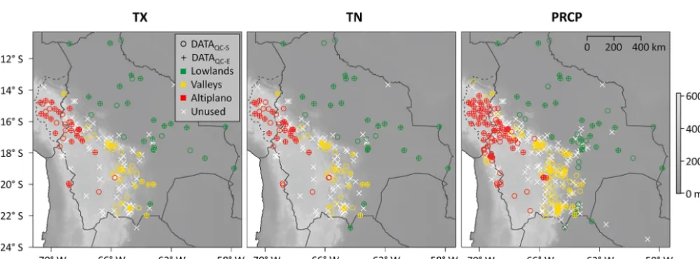
The dataset used for the present study includes observational records from Bolivia (Servicio Nacional de Meteorología e Hidrología de Bolivia, and the Bolivian civil airport adminis-tration), the Peruvian department of Puno (Servicio Nacional de Meteorología e Hidrologí a del Perú), and selected Chilean and Paraguayan stations located near the Bolivian border (Dirección Meteorológica de Chile, Dirección de Me-teorología e Hidrología – Paraguay; Fig. 1). The dataset was created within the framework of the project “Data on climate and Extreme weather for the Central AnDEs” (DECADE) and includes daily TX, TN, and PRCP measurements ((http://www.geography.unibe.ch/research/climatology_ group/research_projects/decade/index_eng.html)). All records in the DECADE dataset originate from manned weather stations. This reflects the conditions of weather observation networks in the Central Andean area where only a few automatic weather stations are in service (Hunziker et al., 2017). The first records in the DECADE dataset date back to 1917, and the most recent observations were taken in 2015. For more details on weather observations in the Central Andean region, see Hunziker et al. (2017).

The altitude of the stations in the study area ranges between 98 and 4667 m a.s.l. Stations at elevations ≤600 m a.s.l. group in the east (henceforward referred to as “lowland stations”), while stations at elevations ≥3500 m a.s.l. are located in the west (henceforward referred to as “Altiplano stations”; see Fig. 1). Stations at altitudes between the lowlands and the Altiplano are grouped along the eastern slopes of the Central Andes and are henceforward referred to as “valley stations”.

Figure 1.Stations of the DECADE dataset with ≥20 years of valid observations for maximum temperature (TX), minimum temperature (TN), and precipitation (PRCP). Solid lines represent country borders, and the dashed line is the border of the Peruvian department of Puno. Circles and pluses indicate stations with ≥80 % of valid measurements from 1981 to 2010 in the datasets quality controlled with a standard method (DATAQC-S) and with an enhanced approach (DATAQC-E), respectively. White crosses mark stations with<80 % of valid observations from 1981 to 2010 in both datasets. Colours classify stations regarding their elevation in lowlands (≤600 m a.s.l.), valleys (601 to 3499 m a.s.l.), and Altiplano (≥3500 m a.s.l.). The grey background shading indicates the elevation in m a.s.l.

and TN and 378 PRCP records. This dataset containing the raw data (i.e. not quality controlled or homogenized) is called “DATARAW” henceforward.

For the present study, all time series of DATARAW were quality controlled and homogenized. However, for the sub-sequent analyses (i.e. error frequency, correlation, and trend analyses), only the period 1981 to 2010 was analysed. During this 30-year standard period, the highest number of station records is available (104 TX, 106 TN, and 220 PRCP time series with≥80 % of valid observations), and data quality is usually higher than earlier in time.

3 Methods

3.1 Quality control

DATARAW was quality controlled with two different ap-proaches. The first approach represents an established stan-dard QC method. Such methods mostly focus on the detec-tion of single suspicious values (Hunziker et al., 2017). The second approach additionally takes systematically occurring data quality issues into account that may remain undetected with standard QC. It is therefore considered as enhanced QC.

3.1.1 Standard approach

The Global Historical Climatology Network GHCN-Daily was developed for a wide range of applications, including studies of extreme events (Menne et al., 2012), and it is the premier source of daily TX, TN, and PRCP observations from various regions of the globe (Donat et al., 2013a). The GHCN-Daily data are quality controlled with a

comprehen-sive set of 19 QC tests, including spatial consistency tests (Durre et al., 2010). It is a fully automatic QC approach that was particularly developed to run unsupervised (Menne et al., 2012). Evaluations of the performance showed that the method is effective at detecting gross errors and more subtle inconsistencies with a low false-positive rate (Durre et al., 2010). This QC method was applied to DATARAW (http://www.geography.unibe.ch/research/climatology_ group/research_projects/decade/index_eng.html).

this practice (even though not ideal) does not introduce any error or bias as long as it remains unchanged. As a conse-quence, internal consistency flags that were set because of this particular QC test were regarded as invalid.

Furthermore, the GHCN-Daily QC did not flag a few ex-treme outliers. This may happen if a reported value exceeds the maximum of five places in tens of degrees Celsius or mil-limetres allowed in the GHCN-Daily data format (e.g. values ≤ −10 000). In order to remove such erroneous numbers, we added an additional flag to all unflagged temperature values >70◦C and<−70◦C and to all unflagged negative PRCP values.

In total, about 0.35 % (temperature) and 0.15 % (PRCP) of all measurements were flagged. This is similar to the over-all fraction of 0.24 % flagged observations in the GHCN-Daily dataset (Durre et al., 2010). In DATARAW, about two-thirds of the flagged temperature and the great majority of the flagged PRCP observations are monthly or yearly dupli-cate data. For any further analyses, all flagged values were removed. The dataset quality controlled with this standard QC approach will be called “DATAQC-S” henceforward.

3.1.2 Enhanced approach

Following the suggestions by Hunziker et al. (2017), DATARAW was carefully checked for systematically oc-curring data quality issues. An extensive set of tests (11 for TX and TN, 15 for PRCP) was applied, and flags were set for each test on an annual timescale (http://www.geography.unibe.ch/research/climatology_ group/research_projects/decade/index_eng.html). Thanks to flagging each quality issue individually in the database, specific time series segments can subsequently be selected that are adequate for the intended purpose. Furthermore, for a segment of one station record (TN of Progreso in Peru; see Hunziker et al., 2017), daily corrections were calculated, since the origin of the correctable error was unambiguously identified.

Time series segments affected by data quality issues that disturb the calculation of monthly means (temperature) and sums (PRCP) were removed from further analyses, which reduced the number of valid measurements by about 40 %. Table 1 briefly describes the data quality issues and related thresholds that led to the exclusion of time series segments. Thresholds were chosen so that quality problems that may significantly affect the subsequent climatological analyses are excluded, whereas data containing minor problems still remain in the dataset. Note that the QC tests were applied in parallel, and therefore time series segments may be affected by several data quality issues simultaneously. If suspicious data patterns could not clearly be attributed to a specific data quality issue, they were classified as “irregularities in the data pattern”. For details on most of the data quality issues in-cluded in the present study, see Hunziker et al. (2017).

Some data quality issues may significantly affect daily ob-servations, but they may lose their significance by monthly aggregation. This particularly applies to observations af-fected by multi-day PRCP accumulations. Such data may still be adequate to calculate monthly totals (WMO, 2011) but cannot be used on a daily timescale (Viney and Bates, 2004). Therefore, more rigorous thresholds were used for data quality issues that cause multi-day PRCP accumulations (i.e. “small PRCP gaps” and “weekly PRCP cycles”) if the data were later analysed on a daily timescale (Table 1). In the present study, daily data are used to analyse the correlation on a daily scale (Sect. 3.3) and the climate change indices (Sect. 3.5).

The QC tests suggested by Hunziker et al. (2017) detect data quality issues that occur systematically during longer time periods (months to years). Therefore, they are not a self-contained QC approach and should be combined with other tests. That is why the GHCN-Daily QC was additionally ap-plied (see Sect. 3.1.1) after removing time series segments of insufficient quality for monthly aggregation. The GHCN-Daily QC added flags to approximately 0.26 % (temperature) and 0.10 % (PRCP) of the remaining observations.

This QC procedure may be considered as an enhancement of applying the GHCN-Daily QC only. Hence, the resulting dataset will be named “DATAQC-E” henceforward.

Note that Hunziker et al. (2017) further suggest the inclu-sion of additional information derived from metadata into the QC process. This allows for the removal of station records that were generated under inappropriate conditions, such as poor station siting or severe lack of station maintenance. The present study, however, only considers quality issues and er-rors that are directly detectable in the measurement data. Hence, time series of questionable quality that could be re-moved by including metadata in the QC process remain in the dataset.

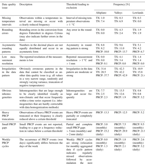
Table 1. Description of systematic data quality issues and their frequencies in the DECADE database (station records with≥20 years of observations) between 1981 and 2010. If not specified, the frequencies of data quality issues apply to daily observations and monthly aggregations. Frequencies of the data quality issues in maximum (TX) and minimum (TN) temperature and precipitation (PRCP) observations are shown for the different regions (Altiplano, valleys, and lowlands; see Fig. 1). Thresholds leading to the exclusion of data were chosen so that data quality issues should not affect the subsequent climatological analyses of the daily and monthly aggregated data. For other analyses, these thresholds may not be adequate and consequently the frequencies of relevant data quality issues may differ. Tests were done in parallel, and time series segments may therefore be affected by several data quality issues simultaneously. For a detailed description of frequent data quality issues, see Hunziker et al. (2017).

Data quality issue

Description Threshold leading to

exclusion

Frequency [%]

Altiplano Valleys Lowlands

Missing temperature intervals

Observations within a temperature in-terval are missing or occur with a clearly reduced frequency

Interval of missing tem-perature observations >1 ◦C

TX: 1.0 TN: 7.4 TX: 0.3 TN: 6.9 TX: 0.3 TN: 0.0 Rounding errors

Rounding errors in the conversion from degrees Fahrenheit to degrees Celsius (may also indicate further errors in the data)

Any error in the round-ing TX: 0.0 TN: 0.0 TX: 4.3 TN: 2.4 TX: 1.9 TN: 1.9 Asymmetric rounding patterns

Numbers in the decimal places are not equally distributed and occur in an asymmetric form

Asymmetry in round-ing pattern is strong

TX: 8.8 TN: 8.2 PRCP: 10.0 TX: 9.6 TN: 11.0 PRCP: 13.7 TX: 5.1 TN: 4.2 PRCP: 6.7 Low mea-surement resolution

The reported resolution of the measure-ments is low

Reported measurement resolution >1◦C and >1 mm

TX: 0.0 TN: 0.0 PRCP: 0.1 TX: 4.1 TN: 3.4 PRCP: 0.0 TX: 1.4 TN: 1.4 PRCP: 0.0 Irregularities in the data pattern

Obviously erroneous patterns in the data that cannot be classified as an-other data quality issue (e.g. all values in a very narrow range, randomly and strongly varying variance, truncation of negative temperatures)

Irregularities in the data pattern are moderate or strong TX: 31.6 TN: 28.5 PRCP: 37.7 TX: 42.3 TN: 42.2 PRCP: 42.9 TX: 10.9 TN: 15.8 PRCP: 21.4 Obvious inhomo-geneities

Inhomogeneities that are large enough to be clearly identified visually as non-climatic and that occur frequently within a time series segment (i.e. inho-mogeneities that are hardly correctable with data homogenization methods)

Inhomogeneities are large and occur fre-quently TX: 7.7 TN: 2.5 PRCP: 2.3 TX: 13.5 TN: 12.6 PRCP: 1.9 TX: 0.8 TN: 0.8 PRCP: 3.2 Heavy PRCP truncations

Observations of heavy PRCP events are truncated or their frequency is clearly reduced above a certain threshold

Heavy PRCP events are partially or completely truncated

PRCP: 13.3 PRCP: 12.5 PRCP: 5.2

Small PRCP gaps

Small PRCP events are not reported, leading to a gap or a frequency reduc-tion in values below a certain threshold

Partial and complete small PRCP gaps >5 mm (monthly) and >2 mm (daily)

PRCP: 3.0 (monthly) PRCP: 15.2 (daily) PRCP: 7.5 (monthly) PRCP: 29.9 (daily) PRCP: 9.5 (monthly) PRCP: 21.9 (daily) Weekly PRCP cycles

The occurrence of PRCP events (wet days) significantly differs between the days of the week

(PRCP) were calculated based on monthly values, and yearly values were calculated only if 12 valid months were available (WMO, 2011).

For many datasets and studies, gaps in time series are filled (e.g. Auer et al., 2007; Kizza et al., 2012; Vuille et al., 2000). There are many techniques for data estimation (e.g. WMO, 2011) that may increase the time series complete-ness and hence the data availability. However, data estima-tion is difficult to apply to Central Andean staestima-tion records due to complex topography, sparse station networks, and mostly few observed atmospheric variables. Furthermore, the input data for ACMANT3 (homogenization method used in the present study; see Sect. 3.4.2) should not include estimated data (Domonkos and Coll, 2017). Hence, in order to avoid in-troducing uncertainty by filling gaps, no data were estimated for the present study.

3.3 Correlation analysis

Before calculating the correlation coefficient of station pairs, time series were standardized by subtracting the mean and dividing by the standard deviation (SD). In order to remove the influence of trends and inhomogeneities, the differences between one observation and the next were calculated. From these time series of the first differences, Spearman rank cor-relations were computed for the period 1981 to 2010.

For correlations on the monthly timescale, daily observa-tions were aggregated as described in Sect. 3.2. Only time se-ries containing≥80 % of valid monthly values in the 30-year period of interest were considered. Removing the flagged ob-servations and time series without sufficient data resulted in 98 (TX), 99 (TN), and 218 (PRCP) valid monthly station records for DATAQC-S and in 56 (TX), 54 (TN), and 105 (PRCP) valid monthly time series for DATAQC-E.

To standardize measurement values on a daily timescale, daily means and SDs were calculated based on the linear in-terpolation of monthly means and SDs. If equal values oc-curred in succession in the original observations, the first dif-ferences of the standardized values were set to zero in order to not bias correlation coefficients by the seasonality of the standardization.

Because unreported shifting of dates occurs frequently in the Central Andean observation networks (Hunziker et al., 2017), temporal dislocation in daily time series pairs must be considered. For example, a high correlation of two Cen-tral Andean time series of the first differences often becomes slightly negative if one of the two time series is shifted by 1 day. Therefore, shifts of −2 to+2 days were applied to one time series of each station pair, and the highest corre-lation value was expected to be the real correcorre-lation coeffi-cient. This method may artificially increase correlations that are close to zero or negative in reality. However, such low correlations are not of interest in the present study. Further-more, we use the median to quantify the effect of data qual-ity issues on correlations, which eliminates the potential bias

introduced to low correlations. Time series with<80 % of daily observations in the period 1981 to 2010 were removed from the daily correlation analysis. This resulted in 104 (TX), 106 (TN), and 220 (PRCP) valid daily station records avail-able for DATAQC-Sand in 59 (TX), 58 (TN), and 90 (PRCP) records for DATAQC-E.

3.4 Data homogenization 3.4.1 Clustering

In order to build station groups that share a similar back-ground climate, we applied agglomerative hierarchical clus-tering with complete linkage on the monthly station cor-relation matrices (see Sect. 3.3). Time series that did not share ≥120 common valid months with ≥10 neighbours were removed from the data homogenization process. For the break detection and adjustment method used in this study (Sect. 3.4.2), the optimal cluster size is usually around 20 to 30 stations, but the optimal number of stations can be much higher if record lengths and data completeness differ between the time series (Domonkos and Coll, 2017). This strongly ap-plies to the Central Andean data. Therefore, we selected three clusters for TX and TN with a median size of 60 (DATAQC-S) and 40 (DATAQC-E) stations. For PRCP, 6 (DATAQC-S) and 5 (DATAQC-E) clusters were selected with a median cluster size of 65 (DATAQC-S) and 42 (DATAQC-E). The minimum and maximum cluster size is 11 and 94 stations, respectively. The spatial structure of the clusters is similar for DATAQC-Sand DATAQC-E. For temperature, two main clus-ters were detected, representing the lowlands and the Alti-plano. Stations of the third cluster are located mostly along the eastern Andean slopes. Spatial illustrations of the clusters are shown in Fig. S1 in the Supplement.

3.4.2 Break-point detection and adjustment

ACMANT3 includes a recommended function for detect-ing monthly outliers that was applied before detectdetect-ing and correcting break points. About twice as many monthly out-liers were detected in DATAQC-S than in DATAQC-E. The highest frequency of monthly outliers was found in TN of DATAQC-S with 0.16 outliers per decade. All monthly out-liers were removed from DATAQC-Sand DATAQC-E.

3.5 Trend calculation

Trends of annual values and climate change indices were analysed for the entire study area in the 30-year time period 1981 to 2010. However, trend signals differ between the var-ied climate zones covered by the DECADE dataset. Thefore, we decided to focus particularly on the Altiplano re-gion for trend analyses. Time series from the Altiplano that satisfy the completeness requirements originate nearly exclu-sively from stations located in the north-western Bolivian de-partment of La Paz and the adjacent Peruvian dede-partment of Puno. In this spatially limited region, the station network is dense compared to the rest of the study area (Fig. 1). There-fore, relatively homogeneous trend signals may be expected. The magnitudes of linear trends were calculated with the Theil–Sen estimator, which is the median of the slopes of all data pairs of a time series (Sen, 1968; Theil, 1950). The method is more insensitive to outliers and more robust than other trend estimators such as ordinary least squares. For individual station records, the significance of trends is not of major interest in the present study and was therefore not tested. Furthermore, taking serial correlation into account in trend tests would cause large uncertainties due to the missing values in the time series. However, for the Altiplano stations, trends of spatially averaged anomalies were tested with the Mann–Kendall test at the 5 % significance level. Before ap-plying the Mann–Kendall test (Mann, 1945; Kendall, 1948), the time series were pre-whitened (Wang and Swail, 2001; Zhang and Zwiers, 2004) in order to remove the influence of serial correlation.

Trends of annual means (temperature) and sums (PRCP) were analysed based on yearly aggregated data (see Sect. 3.2). Time series with <80 % of valid yearly values from 1981 to 2010 were removed previously. This resulted in 54 (TX), 48 (TN), and 105 (PRCP) valid annual station records for DATAQC-S and in 40 (TX), 29 (TN), and 48 (PRCP) annual time series for DATAQC-E.

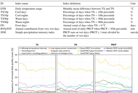
In order to investigate the effect of undetected data quality issues on extremes, we computed the frequently used climate change indices defined by the CCl/CLIVAR/JCOMM Ex-pert Team on Climate Change Detection and Indices (ETC-CDI; http://etccdi.pacificclimate.org/list_27_indices.shtml) for 1981 to 2010. For the calculation of the indices, we used the software tool RClimDex (Zhang and Yang, 2004) that is often applied in climatological studies (e.g. Kioutsioukis et al., 2010; Kruger and Sekele, 2013; New et al., 2006). RClimDex calculates monthly (yearly) index values if ≤3

(≤15) observations are missing (Zhang and Yang, 2004). The indices discussed in the present study are namely the diurnal temperature range (DTR), cool days (TX10p), cool nights (TN10p), warm days (TX90p), warm nights (TN90p), frost days (FD), annual contribution from very wet days (R95pTOT), and the simple daily intensity index (SDII; Ta-ble 2). Note that all indices were calculated on an annual scale. For indices based on percentiles, the baseline period was calculated from the 30-year period 1981 to 2010. Indices units in percentage were converted to days per year.

The ETCCDI climate change indices describe moderate to very moderate extreme events that occur usually many times per year. Therefore, they are particularly suitable for appli-cation on short time series. For the index calculation of the homogenized datasets, daily measurements were corrected by adding monthly adjustment values (temperature) and by multiplying with monthly adjustment factors (PRCP) that were computed with ACMANT3. Applying monthly cor-rections on a time series does not guarantee homogeneity on a daily timescale (Brönnimann, 2015; Costa and Soares, 2009; Trewin, 2013). However, since the present study aims to compare the effects of different QC methods, potential deficits in adjusting daily observations with monthly factors do not bias the results. Considering the large and frequent inhomogeneities detected in the Central Andean time series (Sect. 4.3), the homogeneity of the ETCCDI climate change indices will most likely be increased strongly by correcting the daily time series with the monthly adjustment values.

Trends of the ETCCDI climate change indices were only calculated for time series with ≥80 % of valid yearly in-dex values in the period 1981 to 2010. For the analyses of the climate change indices, about 50 (DATAQC-S) and 30 (DATAQC-E) valid time series for the temperature-derived in-dices (TX10P, TX90P, TN10P, TN90P, and FD) were avail-able. For DTR, which depends on both TX and TN ob-servations, 41 (DATAQC-S) and 22 (DATAQC-E) time series could be analysed. For the PRCP-derived indices SDII and R95pTOT, 106 (DATAQC-S) and 38 (DATAQC-E) indices time series were available.

4 Results

4.1 Frequency of data quality issues

Table 2.ETCCDI climate change indices analysed in the present study. Note that all indices were calculated on an annual timescale. Index units in percentage were converted to days per year in the following analyses.

ID Index name Index definition Unit

DTR Daily temperature range Monthly mean difference between TX and TN ◦C

TX10p Cool days Percentage of days when TX<10th percentile %

TN10p Cool nights Percentage of days when TN<10th percentile %

TX90p Warm days Percentage of days when TX>90th percentile %

TN90p Warm nights Percentage of days when TN>90th percentile %

FD Frost days Annual count of days when TN<0◦C days

R95pTOT Annual contribution from very wet days Annual total of daily PRCP when PRCP>95th percentile mm SDII Simple precipitation intensity index PRCP sum on wet days (PRCP≥1 mm) divided by mm day−1

the number of wet days

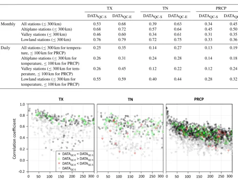
Figure 2. Annual frequency of the data quality issues that cause the exclusion of the affected time series segments for maximum and minimum temperature (TX and TN, respectively) and precipitation (PRCP). If not specified, the frequencies apply to daily observations and monthly aggregations. Note that tests for systematic data quality issues were done in parallel, and time series segments may therefore be affected by several quality issues simultaneously.

regions, and they generally receive less attention from the network operators than other stations in the network.

Some systematic data quality issues are relevant in one re-gion, but not in another. For instance, the “missing tempera-ture intervals” are important in TN observations in the Alti-plano and the valleys, but barely occur in the lowlands. This problem usually occurs in measurements around 0◦C. Tem-peratures in the lowlands rarely drop to the freezing point, and hence this issue is largely absent. In contrast, “weekly PRCP cycles” occur particularly often in the lowlands where the fraction of observations at airports is large (secondary airports are usually out of service on Sundays).

The data quality issue “irregularities in the data pattern” reaches the threshold for exclusion of time series segments more often than the other quality problems. This error classi-fication combines all suspicious data patterns that cannot be clearly classified as another quality issue. In contrast to other data quality issues, irregularities in the data pattern occur in all regions. Time series segments of low quality are often

affected by several problems simultaneously, which usually includes rather unspecific irregularities in the data pattern.

Overall, the quality of the TX, TN, and particularly PRCP observations has slightly increased in the last decades (Fig. 2). However, the frequency of some data quality is-sues has increased, such as strong “asymmetric rounding pat-terns” in TX and TN observations, and “missing temperature intervals” in TN time series. There is no strong or abrupt change in the frequency of the data quality issues between 1981 and 2010. The same applies to the temporal develop-ment of data quality issues in the single regions Altiplano, valleys, and lowlands (not shown).

4.2 Correlation analysis

Table 3.Monthly and daily median correlation coefficients of station pairs within a 300 km radius (100 km for daily PRCP) for maximum temperature (TX), minimum temperature (TN), and precipitation (PRCP).

TX TN PRCP

DATA_QC-S DATA_QC-E DATA_QC-S DATA_QC-E DATA_QC-S DATA_QC-E

Monthly All stations (≤300 km) 0.53 0.68 0.39 0.63 0.34 0.45

Altiplano stations (≤300 km) 0.68 0.72 0.57 0.64 0.45 0.50

Valley stations (≤300 km) 0.46 0.60 0.34 0.61 0.31 0.35

Lowland stations (≤300 km) 0.76 0.79 0.72 0.75 0.33 0.36

Daily All stations (≤300 km for

tempera-ture,≤100 km for PRCP)

0.25 0.35 0.14 0.27 0.13 0.19

Altiplano stations (≤300 km for

temperature,≤100 km for PRCP)

0.26 0.31 0.24 0.28 0.14 0.18

Valley stations (≤300 km for

tem-perature,≤100 km for PRCP)

0.26 0.45 0.12 0.22 0.12 0.24

Lowland stations (≤300 km for

temperature,≤100 km for PRCP)

0.55 0.59 0.40 0.44 0.28 0.32

Figure 3.Correlation coefficients of station pairs as a function of station distance for maximum temperature (TX), minimum temperature (TN), and precipitation (PRCP). This figure shows the example of monthly correlations in the Altiplano (≥3500 m a.s.l.). Black circles indicate equal correlation coefficients in DATAQC-Sand DATAQC-E(absolute difference≤0.01), grey circles indicate correlation coefficients of station combinations of DATAQC-Sthat do not occur in DATAQC-E(or the absolute difference to the equivalent in DATAQC-Eis>0.01), green triangles show correlation coefficients of DATAQC-Ethat are higher than in DATAQC-S(difference>+0.01), and red triangles show correlation coefficients of DATAQC-Ethat are lower than DATAQC-S(difference<−0.01).

than the standard QC approach. While highly correlated sta-tion records remain in DATAQC-E, the enhanced QC largely removes the low correlation coefficients found in DATAQC-S (Fig. 3). Hence, data quality issues that are undetected by the standard QC method result in low correlation coefficients of station pairs. On the other hand, the correlations of sta-tion pairs may change if rather short time series segments are removed due to data quality problems. Usually, this re-sults in an increase in the correlation coefficients (Fig. 3), which may reach up to 0.07 (TX) and 0.09 (PRCP) on a monthly and daily timescale. For TN, maximum corre-lation improvements are 0.10 and 0.05 on a monthly and a daily timescale, respectively. Since this study only includes

time series with≥80 % of valid values, each time series pair shares ≥60 % of common observations between 1981 and 2010 (i.e.≥18 years).

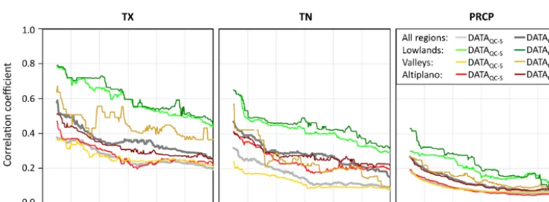
Figure 4.Monthly median correlation coefficients within a 49 km running window for maximum temperature (TX), minimum temperature (TN), and precipitation (PRCP). The median correlation coefficient is not shown if there are less than three station pairs within the running window. Colours mark the medians for all regions combined, the lowlands (≤600 m a.s.l.), the valleys (601 to 3499 m a.s.l.), and the Altiplano (≥3500 m a.s.l.). Light and dark colours indicate correlation coefficients derived from DATAQC-Sand DATAQC-E, respectively.

Figure 5.Same as Fig. 4 but for daily data.

analysed. The resulting median correlation difference for daily PRCP between DATAQC-Eand DATAQC-Sis 0.06.

However, the effect of undetected data quality issues on station correlations varies strongly between the different re-gions. While it is small in the lowlands, it is very pronounced in the valleys. This can be partly explained by the high frac-tion of stafrac-tion records affected by severe data quality issues in the valleys. Lowland stations, in contrast, are often located at airports where data quality problems occur less frequently. There are remarkable differences between the median cor-relation coefficients of station pairs in the lowlands, the val-leys, and the Altiplano (Figs. 4 and 5, Table 3). This is pri-marily explained by the varied topography. While the low-lands are largely flat, the topography of the Altiplano and the valleys is moderately and highly complex, respectively. Therefore, the median correlations are overall highest in the lowlands and lowest in the valleys.

Table 4.Break-point frequencies and break sizes. For minimum and maximum temperature (TX and TN, respectively), absolute break size values in◦C are shown. For precipitation (PRCP), the factors of the break sizes are indicated.

TX TN PRCP

DATAQC-S DATAQC-E DATAQC-S DATAQC-E DATAQC-S DATAQC-E

Break points per decade 1.0 0.9 1.1 0.9 0.3 0.2

Median absolute break-point size 1.1◦C 0.8◦C 1.1◦C 0.8◦C 1.25 1.15

Mean absolute break-point size 1.5◦C 1.0◦C 1.6◦C 1.2◦C 1.30 1.20

Maximum absolute break-point size 10.2◦C 5.0◦C 8.4◦C 5.0◦C 3.40 2.00

Figure 6.Kernel density of the adjustments calculated with ACMANT3 for all regions and the complete time series(a)and for the Altiplano stations from 1981 to 2010(b). For maximum and minimum temperature (TX and TN, respectively), inhomogeneous time series segments are corrected by adding the adjustment values, whereas for precipitation (PRCP), inhomogeneous segments are corrected by multiplication with the adjustment factors.

correlation coefficients of daily observations in the lowlands. Note, however, that the correlation differences between the regions are more pronounced within DATAQC-Sthan within DATAQC-E.

4.3 Data homogenization

One out of three TN station clusters of DATAQC-S(34 sta-tion records) could not be homogenized because of too-low spatial–temporal coherence. Most of the time series in this cluster are affected by systematic data quality issues that were not detected with the standard QC approach. Since these station records could not be homogenized, they were excluded from all further analyses.

ACMANT3 detected a high number of break points in the station records. For temperature, about one break point per decade was detected on average, with a slightly higher break-point frequency in DATAQC-Sthan in DATAQC-E (Ta-ble 4). For PRCP, 0.3 break points per decade were found in DATAQC-Sand 0.2 in DATAQC-E. Median, mean, and

maxi-mum break-point sizes are clearly larger in DATAQC-Sthan in DATAQC-Efor all climate variables (Table 4).

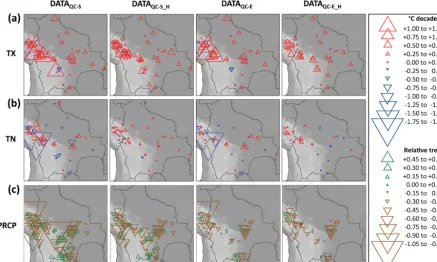
Figure 7. Trends of individual station records for maximum temperature (TX)(a), minimum temperature (TN) (b), and precipitation (PRCP)(c)from 1981 to 2010. The first column shows the results for the unhomogenized dataset quality controlled with the standard approach (DATAQC-S), the second column shows the homogenized dataset quality controlled with the standard approach (DATAQC-S_H), the third column shows the unhomogenized dataset quality controlled with the enhanced approach (DATAQC-E), and the fourth column shows the homogenized dataset quality controlled with the enhanced approach (DATA_{QC-E_H}). For temperature, trends are indicated in◦C per decade. For PRCP, the relative magnitudes of the trend changes from 1981 to 2010 are shown. They are calculated from the difference between the fitted value at the end and the beginning of the time series, which is divided by the mean of the fit. A relative trend increase by 1 is equal to an increase by 200.0 %, and a relative decrease by 1 is equal to a decrease by 66.7 %.

Henceforward, the homogenized datasets DATAQC-Sand DATAQC-E are named “DATAQC-S_H” and “DATAQC-E_H”, respectively. Note that some time series segments could not be homogenized due to lacking reference stations with the required correlation. For the trend analyses, all time se-ries segments that remained unhomogenized were also ex-cluded from the unhomogenized datasets (i.e. DATAQC-Sand DATAQC-E) in order to maintain comparability between un-homogenized and un-homogenized datasets.

4.4 Trends

4.4.1 Annual temperature averages

Overall, there is a clear positive TX trend in the entire study area (Fig. 7). The few negative TX trends in the unhomoge-nized station records disappear due to data homogenization. In the Altiplano, the trend of the spatially averaged anoma-lies is significant and varies between+0.40 (DATAQC-E_H) and+0.44◦C (DATAQC-E) per decade (Table 5). TN trends, however, are more ambiguous. Spatial trend patterns are un-clear, except for DATAQC-E_H in which a clear warming is found in the north-eastern Altiplano and slight cooling in the

south and the lowlands. This pattern is spatially coherent and substantially diverges from the spatial trend patterns derived from the other datasets. As a result, TN trends of spatially averaged anomalies calculated from DATAQC-E_Hin the Alti-plano are significant with+0.22◦C per decade, whereas they are close to zero and insignificant if calculated from the other datasets (Table 5). This may be at least partly ascribed to the results of the data homogenization process, which suggest a clear overall warm bias in earlier TN observations in the Altiplano in DATAQC-E, but not in DATAQC-S(Sect. 4.3).

Table 5.Trends of spatially averaged anomalies in the Altiplano (≥3500 m a.s.l.) in the period 1981 to 2010. Trends are shown for the annual means, for the 10th and 90th percentile of maximum temperature (TX) and minimum temperature (TN; i.e. TX10p, TN10p, TX90p, TN90p), and for the number of frost days (FD). Bold numbers denote significance at the 5 % level.

TX TN

DATA DATA DATA DATA DATA DATA DATA DATA

QC-S QC-S_H QC-E QC-E_H QC-S QC-S_H QC-E QC-E_H Annual means (◦C decade−1) +0.41 +0.42 +0.44 +0.40 −0.04 +0.05 −0.12 +0.22 10th percentile (days decade−1) −13.2 −14.4 −12.0 −11.9 +0.4 −1.0 −0.9 −5.8 90th percentile (days decade−1) +8.7 +11.0 +9.8 +9.3 +0.2 +3.7 +2.0 +8.8

FD (days decade−1) – – – – +2.9 −1.3 +1.4 −6.5

Figure 8.Trends of individual station records for maximum temperature (TX), minimum temperature (TN), and precipitation (PRCP) in the period 1981 to 2010. Trend box plots for the complete study area and for the Altiplano (≥3500 m a.s.l.) are shown. Colours indicate the different datasets that are unhomogenized and quality controlled with the standard approach (DATAQC-S), homogenized and quality controlled with the standard approach (DATAQC-S_H), unhomogenized and quality controlled with the enhanced approach (DATAQC-E), and homogenized and quality controlled with the enhanced approach (DATA_{QC-E_H}). For temperature, trends are specified in◦C per decade. For PRCP, relative trends from 1980 to 2010 are shown (see the caption of Fig. 7 for details). The box plots show the median, the 25th and 75th percentile, and the 1.5×IQR (whiskers).

4.4.2 Annual precipitation sums

PRCP trends are negative for most station records (Fig. 7). The spatial pattern of trend magnitudes is more coherent if trends are calculated from DATAQC-E_Hthan from the other datasets. Despite the previous homogenization of the time series in DATAQC-S_H, there are strong positive and nega-tive trends of stations within a short distance. For all regions (lowlands, valleys, and Altiplano), trends of the spatially av-eraged anomalies are negative, particularly if derived from DATAQC-E_H (not shown). However, these trends are barely significant due to the high interannual variability of PRCP.

The trend spread and frequency of very strong trends is lower in DATAQC-Ethan in DATAQC-S(Fig. 8). Data homog-enization reduces the trend spread of the PRCP time series,

but considerably less than for temperature data. Overall, the spread of PRCP trends of individual station records is rela-tively large in all datasets.

4.4.3 Climate change indices

re-Figure 9.Trends of individual station records of the complete study area for the climate change indices daily temperature range (DTR), number of cool days (TX10p), number of warm days (TX90p), number of cool nights (TN10p), and number of warm nights (TN90p) in the period 1981 to 2010. Colours indicate the different datasets that are unhomogenized and quality controlled with the standard approach (DATAQC-S), homogenized and quality controlled with the standard approach (DATAQC-S_H), unhomogenized and quality controlled with the enhanced approach (DATAQC-E), and homogenized and quality controlled with the enhanced approach (DATAQC-E_H). For the DTR, trends are specified in◦C per decade and for the other indices in days per decade. The box plots show the median, the 25th and 75th percentile, and the 1.5×IQR (whiskers).

Figure 10.Same as Fig. 9 but for the Altiplano stations (≥3500 m a.s.l.). Additionally, trends of frost days (FD) are shown.

duced to a range between +0.10 and+0.29◦C per decade (Fig. 10). Besides this high DTR trend coherency derived from DATAQC-E_H in the Altiplano, trend magnitudes are clearly lower than those derived from the other datasets. This manifests in an insignificant trend of the spatially averaged anomalies of+0.23◦C per decade for DATAQC-E_H, whereas the trends calculated from the other datasets are all signifi-cant and range between+0.39 (DATAQC-S_H) and+0.54◦C per decade (DATAQC-S).

The overall trend signal of the TX-based percentile in-dices TX10p and TX90p is relatively uniform among the different datasets, indicating a reduction in cool days and

an increase in warm days (Figs. 9 and 10). The trends of the spatially averaged anomalies in the Altiplano calcu-lated from the different datasets are all significant and range between −11.9 (DATAQC-E_H) and −14.4 (DATAQC-S_H) cool days per decade and between +8.7 (DATAQC-S) and +11.0 (DATAQC-S_H) warm days per decade (Table 5). For both indices, the trend magnitudes are more pronounced for DATAQC-S_Hthan for DATAQC-E_H.

trend magnitudes derived from DATAQC-E_H differ substan-tially from the other datasets (Fig. 10) by indicating a clear warming trend in all indices (i.e. decrease in cool nights and frost days, increase in warm nights). This is confirmed by the trends of the spatially averaged anomalies that indicate a significant decrease in cool nights (−5.8 days per decade) and a significant increase in warm nights (+8.8 days per decade; Table 5). In contrast, the trends calculated from the other datasets are all insignificant and have lower trend mag-nitudes. The same pattern is found for trends of the frequency of frost days (FD). Trends calculated from DATAQC-E_H in-dicate a significant decrease in FD (−6.5 days per decade), whereas the trends of the other datasets are insignificant and close to zero (Table 5).

The PRCP-based climate change indices indicate a slight decrease in the annual contribution of very wet days (R95pTOT) and a decreasing intensity of precipitation events (SDII), particularly in the Altiplano. This signal is more pro-nounced for the datasets quality controlled with the standard method than for the datasets quality controlled with the en-hanced approach. Trends of the spatially averaged anoma-lies are not significant, except for the trends of SDII de-rived from the dataset quality controlled with the standard approach in the Altiplano, i.e. −3.1 mm day−1(DATAQC-S) and −2.1 mm day−1 (DATAQC-S_H) per decade. In contrast to the indices derived from temperature data, applying the enhanced QC approach reduces the trend spread of the PRCP-based indices more than statistical data homogeniza-tion. Compared to DATAQC-S, the SDs of the relative trends in the complete study area calculated from DATAQC-S_H, DATAQC-E, and DATAQC-E_Hare 20, 40, and 50 % lower, re-spectively.

5 Discussion

Systematically occurring data quality issues affect a large fraction of Central Andean station records, making about 40 % inadequate for the calculation of monthly means (tem-perature) and sums (PRCP). The frequency of such problems may vary strongly in space and time. Systematic data qual-ity issues remain largely undetected when applying standard data quality control methods such as the one used for the GHCN-Daily database. Hence, important data sources may be substantially affected by such undetected data quality is-sues (abbreviated as UDQIs henceforward). Including tests to specifically detect such erroneous patterns could signifi-cantly increase the quality of many datasets.

On a monthly timescale and up to 300 km of station dis-tance, UDQIs cause a reduction of median correlation co-efficients by 0.15 (TX), 0.24 (TN), and 0.11 (PRCP) com-pared to unaffected data. On a daily timescale, this reduction is 0.10 (TX) and 0.13 (TN) for station pairs within 300 km of distance and 0.06 (PRCP) for stations within 100 km of distance. These findings confirm the assumption by Gubler

et al. (2017) that the strong differences in correlation co-efficients between station networks of the Peruvian Andes and Switzerland may not be explained by unequal climate regimes alone. Hypothesizing that UDQIs occur more fre-quently in the station networks of developing than devel-oped countries, a higher frequency of such errors can be ex-pected in tropical areas than in mid-latitudes. Making this assumption, UDQIs may partly explain the particularly low correlation decay distances in the tropics described by New et al. (2000). Using relatively high minimum correlation thresholds in climatological analyses (e.g. data homogeniza-tion) may reduce the amount of station records affected by UDQIs. As a more advanced approach, weighting correla-tion coefficients with stacorrela-tion distances (i.e. more weight to station pairs further away from each other for equal correla-tion coefficients) could particularly take UDQIs into account. UDQIs induce additional inhomogeneities in observa-tional records. The resulting decrease in the signal-to-noise ratio may decrease the performance of statistical data ho-mogenization methods (Domonkos, 2013). This is particu-larly problematic in sparse observational networks in which a high number of break points may result in adjustments that deteriorate the temporal consistency of station records (Gubler et al., 2017). In the Central Andean region, UDQIs increase the number of statistically detected break points by about 15 % for TX and TN and by 50 % for PRCP. They also increase the median break-point size by 35 to 40 % (TX and TN) and 60 % (RPCP) and increase break size maxima by up to 100 % (temperature) and 70 % (PRCP). Since UDQIs have larger relative effects on break sizes than on the num-ber of detected break points, they apparently deteriorate the detectability of small non-climatic inhomogeneities.

observed adjustment differences of TN records in the Alti-plano. Hence, UDQIs may impede the adjustments of sys-tematic biases introduced by inhomogeneities. In summary, UDQIs may substantially decrease the performance of statis-tical data homogenization methods.

Between 1981 and 2010, a pronounced and relatively uni-form increase in global mean temperatures was observed (IPCC, 2013). Similarly, clear overall warming trends in the same period were reported from analyses of extremes indices (Donat et al., 2013b). Hence, 1981 to 2010 is a suitable pe-riod for analysing linear temperature trends, and clear trend signals may be expected in the Central Andean area too.

UDQIs increase the overall spread of individual station trends. Statistical data homogenization may largely reduce or eliminate this effect, but only at the cost of more and larger break points, which lowers the performance of data enization methods. For instance, the trend spread of homog-enized TN time series quality controlled with the standard approach (DATAQC-S_H) is extremely small (Fig. 8). This clearly deviates from the trend spreads observed for TX and from the trend spread derived from DATAQC-E_H. Hence, sta-tion trends computed from DATAQC-S_Hseem rather implau-sible and may indicate an over-homogenization. In contrast, the low trend spread of the diurnal temperature range (DTR) derived from DATAQC-E_H (Fig. 10) suggests that the inde-pendent data homogenizations of TX and TN observations are consistent with each other. Furthermore, trends calculated from DATAQC-E_H are spatially more coherent than those derived from DATAQC-S_H, particularly for TN and PRCP (Fig. 7).

If datasets contain UDQIs and/or are unhomogenized, TN trends of averaged anomalies in the Altiplano are close to zero and insignificant, and trends of the diurnal tempera-ture range (DTR) are strongly positive and significant at the 5 % level (Table 5). In contrast, TN trends derived from DATAQC-E_H are significantly positive, and trends of the DTR are insignificant. Hence, mean temperature trends in the Altiplano are more in accordance with the global observa-tions (IPCC, 2013) if systematically occurring data quality issues are removed from the dataset. Nevertheless, the in-fluence of UDQIs in station records from the Altiplano ex-plains roughly half of the trend difference between TX and TN. Hence, there must be other factors (climatological or non-climatological) that cause a stronger increase in TX than TN in the Altiplano. An indication of a climatological expla-nation for the positive DTR trend is the simultaneously ob-served negative PRCP trend. Several authors have described a negative correlation between DTR and PRCP trends (Dittus et al., 2014; Jaswal et al., 2016; Zhou et al., 2009). Hence, the observations in the Altiplano would be in accordance with these findings.

Since systematically occurring data quality issues espe-cially affect extremes (Hunziker et al., 2017), UDQIs have a stronger effect on ETCCDI climate change indices than on trends of annual means (temperature) and sums (PRCP).

Particularly in the Altiplano, the spread of individual station trends is usually more coherent if trends are calculated from DATAQC-E_H than from the other datasets. For the climate change indices derived from PRCP analysed in the present study (R95pTOT and SDII), most very strong trends of in-dividual time series are caused by UDQIs and cannot be ad-justed by statistical data homogenization. Hence, highly in-coherent spatial trend signals and strong differences in trend magnitudes between neighbouring stations as detected in many studies (e.g. Skansi et al., 2013; Vuille et al., 2003; You et al., 2011) may potentially be ascribed to UDQIs.

The overall temperature trend signals derived from DATAQC-E_Hin the Altiplano are highly coherent, indicating significant warming throughout all indices. This trend pattern of moderate extreme events is more in accordance with the global observations (e.g. IPCC, 2013) than the trend patterns derived from the other datasets. Consequently, UDQIs may at least partly explain the discrepancies of trends detected in the Altiplano compared to most other world regions.

According to Donat et al. (2013b), gridding observations minimizes the impact of data quality issues at individual stations due to averaging. This, however, may not be true if UDQIs cause systematic biases. We calculated trends of the relevant climate change indices derived from the two 2.5◦×3.75◦grid cells of the HadEX2 dataset (Donat et al., 2013b) that are most representative for the Altiplano. Over-all, these trends in the period 1981 to 2010 are most similar to the trends derived from DATAQC-S_H. However, the trends of a few climate change indices derived from HadEx2 have extreme magnitudes, such as a detected increase of+14.0 frost days per decade in one of the grid cells. Furthermore, virtually all of these trends are insignificant due to large vari-abilities in the annual index time series. Even though these findings do not allow clear conclusions to be drawn, they suggest that UDQIs affect the dataset and influence the trend calculations.

(e.g. Amazonian lowlands), whereas they may significantly bias monthly PRCP sums in rather dry areas (e.g. Altiplano) due to low overall PRCP and evaporation losses. As demon-strated in this work, UDQIs have stronger effects on climato-logical analyses derived from TN than TX observations. On the one hand, TN is generally more variable and spatially het-erogeneous than TX (Luhunga et al., 2014; Mahmood et al., 2006; New et al., 1999). On the other hand, measurement errors may occur more frequently in TN than TX. For exam-ple, TN falls naturally more often below freezing tempera-ture than TX, and temperatempera-ture values around and below 0◦C often trigger measurement errors by observers and data tran-scription errors (Hunziker et al., 2017). Hence, the frequency and effects of UDQIs also vary spatially and temporally.

Removing a relatively large fraction of observations (about 40 % in the present study) from a dataset may affect the re-sults of climatological analyses. Reducing the spatial den-sity of available data normally decreases the quality of the results such as for data homogenization (Caussinus and Mestre, 2004; Domonkos, 2013; Gubler et al., 2017). With the present study, however, we have demonstrated that re-moving time series segments affected by UDQIs increases the overall quality of the dataset, and the results of climato-logical analyses are consequently more coherent and reliable. The disadvantage of fewer available observations is outper-formed by the quality increase in the dataset.

6 Conclusions

Systematically occurring data quality issues may affect large fractions of time series in observational datasets. In the Cen-tral Andean area, about 40 % of the observations are inap-propriate for the calculation of monthly temperature means and precipitation sums. These problems remain largely un-detected by standard quality control methods. In the present study, we applied a standard and an enhanced quality con-trol approach on the same dataset. The enhanced approach should particularly detect systematically occurring data qual-ity issues. We subsequently compared the results of various climatological analyses derived from the dataset quality con-trolled with the two different methods.

Undetected data quality issues (UDQIs) substantially lower the correlation coefficients of station pairs. This di-rectly affects various methods such as clustering or data ho-mogenization.

The performance of data homogenization approaches de-teriorates if time series contain UDQIs. Since UDQIs induce inhomogeneities in time series, they increase the number and average size of break points in the data. As a result of the in-creased noise in the station records, the skill of statistical data homogenization methods to detect and correct smaller inho-mogeneities is reduced. Furthermore, data homogenization approaches may fail to detect and correct systematic biases caused by inhomogeneities due to UDQIs. In the Altiplano,

for instance, a median adjustment value of−0.5◦C for min-imum temperature observations was detected for time series free of UDQIs, whereas a median adjustment of+0.2◦_{C was} computed for the station records affected by UDQIs. This warm bias in earlier TN observations may affect previous studies using station records from the Altiplano. Hence, data homogenization methods rely on data that are largely free of UDQIs in order to perform satisfactorily.

Removing UDQIs from a dataset increases the spatial co-herence and reduces the spread of individual stations trends. Furthermore, UDQIs may systematically bias trends. For in-stance, regional minimum temperature trends in the Alti-plano are insignificant and close to zero if calculated from station records affected by UDQIs, whereas trends are sig-nificant and clearly positive if derived from time series free of UDQIs.

Since UDQIs especially affect extremes, they are partic-ularly problematic for analysing trends of rare events such as for the ETCCDI climate change indices. In the Altiplano, trends of various indices based on minimum temperature dif-fer significantly if derived from a dataset affected or unaf-fected by UDQIs. For some climate change indices based on precipitation, extreme trend magnitudes at individual stations can be corrected by previously removing UDQIs from the dataset, but not by statistical data homogenization.

Most likely, the results of various studies are affected by UDQIs. If quality control approaches are enhanced and UDQIs removed, the results of climatological analyses may become more coherent and reliable. Note that an enhanced and comprehensive quality control cannot substitute for ap-propriate data homogenization and vice versa.

Data availability. The DECADE database including all quality control flags is available under http://www.geography.unibe.ch/ research/climatology_group/research_projects/decade/index_eng. html.

The Supplement related to this article is available online at https://doi.org/10.5194/cp-14-1-2018-supplement.

Competing interests. The authors declare that they have no con-flict of interest.

newest version of RClimDex. We also thank the two anonymous reviewers for their helpful comments and suggestions.

Edited by: Volker Rath

Reviewed by: two anonymous referees

References

Aguilar, E., Auer, I., Brunet, M., Peterson, T. C., and Wieringa, J.: Guidlines on Climate Metadata and Homogenization. in: WCDMP No. 53, WMO/TD No. 1186, World Meteorological Organization, Geneva, Switzerland, 2003.

Alexander, L. V., Zhang, X., Peterson, T. C., Caesar, J., Gleason, B., Klein Tank, A. M. G., Haylock, M., Collins, D., Trewin, B., Rahimzadeh, F., Tagipour, A., Rupa Kumar, K., Revadekar, J., Griffiths, G., Vincent, L., Stephenson, D. B., Burn, J., Aguilar, E., Brunet, M., Taylor, M., New, M., Zhai, P., Rusticucci, M., and Vazquez-Aguirre, J. L.: Global observed changes in daily climate extremes of temperature and precipitation, J. Geophys. Res.-Atmos., 111, D05109, https://doi.org/10.1029/2005JD006290, 2006.

Auer, I., Böhm, R., Jurkovic, A., Lipa, W., Orlik, A., Potz-mann, R., Schöner, W., Ungersböck, M., Matulla, C., Briffa, K., Jones, P., Efthymiadis, D., Brunetti, M., Nanni, T., Maugeri, M., Mercalli, L., Mestre, O., Moisselin, J.-M., Begert, M., Müller-Westermeier, G., Kveton, V., Bochnicek, O., Stastny, P., Lapin, M., Szalai, S., Szentimrey, T., Cegnar, T., Dolinar, M., Gajic-Capka, M., Zaninovic, K., Majstorovic, Z., and Nieplova, E.: HISTALP – historical instrumental climato-logical surface time series of the Greater Alpine Region, Int. J. Climatol., 27, 17–46, https://doi.org/10.1002/joc.1377, 2007. Brönnimann, S.: Climatic Changes Since 1700,

Springer International Publishing, Cham, Switzerland, https://doi.org/10.1007/978-3-319-19042-6_4, 2015.

Cao, L.-J., and Yan, Z.-W.: Progress in research on homogeniza-tion of climate data, Adv. Climate Change Res., 3, 59–67, https://doi.org/10.3724/SP.J.1248.2012.00059, 2012.

Caussinus, H. and Mestre, O.: Detection and correction of artifi-cial shifts in climate series, J. R. Stat. Soc. C, 53, 405–425, https://doi.org/10.1111/j.1467-9876.2004.05155.x, 2004. Costa, A. and Soares, A.: Homogenization of climate data: review

and new perspectives using geostatistics, Math. Geosci., 41, 291– 305, https://doi.org/10.1007/s11004-008-9203-3, 2009. Dittus, A., Karoly, D., C Lewis, S., and Alexander, L.: An

investigation of some unexpected frost day increases in Southern Australia, Aust. Meteorol. Ocean., 64, 261–271, https://doi.org/10.22499/2.6404.002, 2014.

Domonkos, P.: Adapted Caussinus–Mestre Algorithm for Networks of Temperature Series (ACMANT), Int. J. Geosci., 2, 293–309, https://doi.org/10.4236/ijg.2011.23032, 2011.

Domonkos, P.: Homogenization of precipitation time series with ACMANT, Theor. Appl. Climatol., 122, 303–314, https://doi.org/10.1007/s00704-014-1298-5, 2015.

Domonkos, P.: Measuring performances of homogenization meth-ods, Q. J. Hungar. Meteorol. Serv., 117, 91–112, 2013.

Domonkos, P. and Coll, J.: Homogenisation of temperature and precipitation time series with ACMANT3: method descrip-tion and efficiency tests, Int. J. Climatol., 37, 1910–1921, https://doi.org/10.1002/joc.4822, 2017.

Donat, M. G., Alexander, L. V., Yang, H., Durre, I., Vose, R., and Caesar, J.: Global land-based datasets for monitoring climatic extremes, B. Am. Meteorol. Soc., 94, 997–1006, https://doi.org/10.1175/bams-d-12-00109.1, 2013a.

Donat, M. G., Alexander, L. V., Yang, H., Durre, I., Vose, R., Dunn, R. J. H., Willett, K. M., Aguilar, E., Brunet, M., Caesar, J., Hewitson, B., Jack, C., Klein Tank, A. M. G., Kruger, A. C., Marengo, J., Peterson, T. C., Renom, M., Oria Rojas, C., Rus-ticucci, M., Salinger, J., Elrayah, A. S., Sekele, S. S., Srivas-tava, A. K., Trewin, B., Villarroel, C., Vincent, L. A., Zhai, P., Zhang, X., and Kitching, S.: Updated analyses of tempera-ture and precipitation extreme indices since the beginning of the twentieth century: the HadEX2 dataset, J. Geophys. Res.-Atmos., 118, 2098–2118, https://doi.org/10.1002/jgrd.50150, 2013b.

Durre, I., Menne, M. J., Gleason, B. E., Houston, T. G., and Vose, R. S.: Comprehensive automated quality assurance of daily surface observations, J. Appl. Meteorol. Clim., 49, 1615–1633, https://doi.org/10.1175/2010JAMC2375.1, 2010.

Espinoza, J., Ronchail, J., Lengaigne, M., Quispe, N., Silva, Y., Bet-tolli, M., Avalos, G., and Llacza, A.: Revisiting wintertime cold air intrusions at the east of the Andes: propagating features from subtropical Argentina to Peruvian Amazon and relationship with large-scale circulation patterns, Clim. Dynam., 41, 1983–2002, https://doi.org/10.1007/s00382-012-1639-y, 2013.

Garreaud, R. D.: Multiscale analysis of the summertime precipitation over the Central Andes, Mon. Weather Rev., 127, 901–921, https://doi.org/10.1175/1520-0493(1999)127<0901:maotsp>2.0.co;2, 1999.

Garreaud, R. D.: Cold air incursions over subtropical South America: mean structure and dynamics, Mon. Weather Rev., 128, 2544–2559, https://doi.org/10.1175/1520-0493(2000)128<2544:CAIOSS>2.0.CO;2, 2000.

Garreaud, R. D.: Subtropical cold surges: regional aspects and global distribution, Int. J. Climatol., 21, 1181–1197, https://doi.org/10.1002/joc.687, 2001.

Garreaud, R. D.: The Andes climate and weather, Adv. Geosci., 22, 3–11, https://doi.org/10.5194/adgeo-22-3-2009, 2009.

Gubler, S., Hunziker, S., Begert, M., Croci-Maspoli, M., Konzelmann, T., Brönnimann, S., Schwierz, C., Oria, C., and Rosas, G.: The influence of station density on cli-mate data homogenization, Int. J. Climatol., 37, 4670–4683, https://doi.org/10.1002/joc.5114, 2017.

Hunziker, S., Gubler, S., Calle, J., Moreno, I., Andrade, M., Ve-larde, F., Ticona, L., Carrasco, G., Castellón, Y., Oria, C., Croci-Maspoli, M., Konzelmann, T., Rohrer, M., and Brönnimann, S.: Identifying, attributing, and overcoming common data quality is-sues of manned station observations, Int. J. Climatol., 37, 4131– 4145, https://doi.org/10.1002/joc.5037, 2017.

IPCC: Climate Change 2013: The Physical Science Basis, in: Con-tribution of Working Group I to the Fifth Assessment Report of the Intergovernmental Panel on Climate Change, edited by: Stocker, T. F., Qin, D., Plattner, G.-K., Tignor, M., Allen, S. K., Boschung, J., Nauels, A., Xia, Y., Bex, V., and Midgley, P. M., Cambridge University Press, Cambridge, UK and New York, NY, USA, https://doi.org/10.1029/2000JD000115, 2013.

low cloud cover and rainy days, J. Clim. Change, 2, 35–55, https://doi.org/10.3233/JCC-160016, 2016.

Kendall, M. G.: Rank correlation methods, Griffin, London, 1948. Kioutsioukis, I., Melas, D., and Zerefos, C.: Statistical assessment

of changes in climate extremes over Greece (1955–2002), Int. J. Climatol., 30, 1723–1737, https://doi.org/10.1002/joc.2030, 2010.

Kizza, M., Westerberg, I., Rodhe, A., and Ntale, H. K.: Esti-mating areal rainfall over Lake Victoria and its basin using ground-based and satellite data, J. Hydrol., 464–465, 401–411, https://doi.org/10.1016/j.jhydrol.2012.07.024, 2012.

Kruger, A. C. and Sekele, S. S.: Trends in extreme temperature in-dices in South Africa: 1962–2009, Int. J. Climatol., 33, 661–676, https://doi.org/10.1002/joc.3455, 2013.

López-Moreno, J. I., Morán-Tejeda, E., Vicente-Serrano, S. M., Bazo, J., Azorin-Molina, C., Revuelto, J., Sánchez-Lorenzo, A., Navarro-Serrano, F., Aguilar, E., and Chura, O.: Re-cent temperature variability and change in the Altiplano of Bolivia and Peru, Int. J. Climatol., 36, 1773–1796, https://doi.org/10.1002/joc.4459, 2016.

Luhunga, P. M., Mutayoba, E., and Ng’ongolo, H. K.: Homo-geneity of monthly mean air temperature of the United Repub-lic of Tanzania with HOMER, Atmos. Clim. Sci., 4, 70–77, https://doi.org/10.4236/acs.2014.41010, 2014.

Mahmood, R., Foster, S. A., and Logan, D.: The GeoProfile metadata, exposure of instruments, and measurement bias in climatic record revisited, Int. J. Climatol., 26, 1091–1124, https://doi.org/10.1002/joc.1298, 2006.

Mann, H. B.: Nonparametric Tests Against Trend, Econometrica, 13, 245–259, https://doi.org/10.2307/1907187, 1945.

Menne, M. J., Durre, I., Vose, R. S., Gleason, B. E., and Hous-ton, T. G.: An overview of the global historical climatology network-daily database, J. Atmos. Ocean. Tech., 29, 897–910, https://doi.org/10.1175/JTECH-D-11-00103.1, 2012.

Mestre, O., Domonkos, P., Picard, F., Auer, I., Robin, S., Lebar-bier, E., Böhm, R., Aguilar, E., Guijarro, J., Vertachnik, G., Klan-car, M., Dubuisson, B., and Stepanek, P.: HOMER: a homoge-nization software – methods and applications, Q. J. Hungar. Me-teorol. Serv., 117, 47–67, 2013.

Morak, S., Hegerl, G. C., and Kenyon, J.: Detectable regional changes in the number of warm nights, Geophys. Res. Lett., 38, L17703, https://doi.org/10.1029/2011GL048531, 2011. New, M., Hulme, M., and Jones, P.: Representing

twentieth-century space–time climate variability. Part I: Develop-ment of a 1961–90 mean monthly terrestrial climatol-ogy, J. Climate, 12, 829–856, https://doi.org/10.1175/1520-0442(1999)012<0829:RTCSTC>2.0.CO;2, 1999.

New, M., Hulme, M., and Jones, P.: Representing twentieth-century space–time climate variability. Part II: Develop-ment of 1901–96 monthly grids of terrestrial surface cli-mate, J. Clicli-mate, 13, 2217–2238, https://doi.org/10.1175/1520-0442(2000)013<2217:RTCSTC>2.0.CO;2, 2000.

New, M., Hewitson, B., Stephenson, D. B., Tsiga, A., Kruger, A., Manhique, A., Gomez, B., Coelho, C. A. S., Masisi, D. N., Kul-ulanga, E., Mbambalala, E., Adesina, F., Saleh, H., Kanyanga, J., Adosi, J., Bulane, L., Fortunata, L., Mdoka, M. L., and La-joie, R.: Evidence of trends in daily climate extremes over south-ern and west Africa, J. Geophys. Res.-Atmos., 111, D14102, https://doi.org/10.1029/2005JD006289, 2006.

Plummer, N., Allsopp, T., and Lopez, J. A.: Guidelines on Climate Observations Networks and Systems, in: WCDMP No. 53, WMO/TD No. 1186, World Meteorological Organiza-tion, Geneva, Switzerland, 2003.

Quintana-Gomez, R. A.: Trends of maximum and mini-mum temperatures in northern South America, J. Cli-mate, 12, 2104–2112, https://doi.org/10.1175/1520-0442(1999)012<2104:TOMAMT>2.0.CO;2, 1999.

Rhines, A., Tingley, M. P., McKinnon, K. A., and Huy-bers, P.: Decoding the precision of historical temperature observations, Q. J. Roy. Meteorol. Soc., 141, 2923–2933, https://doi.org/10.1002/qj.2612, 2015.

Ribeiro, S., Caineta, J., and Costa, A. C.: Review and discussion of homogenisation methods for climate data, Phys. Chem. Earth, 94, 167–179, https://doi.org/10.1016/j.pce.2015.08.007, 2016. Rosas, G., Gubler, S., Oria, C., Acuña, D., Avalos, G., Begert, M.,

Castillo, E., Croci-Maspoli, M., Cubas, F., Dapozzo, M., Díaz, A., van Geijtenbeek, D., Jacques, M., Konzelmann, T., Lavado, W., Matos, A., Mauchle, F., Rohrer, M., Rossa, A., Scherrer, S. C., Valdez, M., Valverde, M., Villar, G., and Villegas, E.: Towards implementing climate services in Peru – the project CLIMANDES, Climate Services, 4, 30–41, https://doi.org/10.1016/j.cliser.2016.10.001, 2016.

Sen, P. K.: Estimates of the regression coefficient based on Kendall’s Tau, J. Am. Stat. Assoc., 63, 1379–1389, https://doi.org/10.2307/2285891, 1968.

Skansi, M. d. l. M., Brunet, M., Sigró, J., Aguilar, E., Arevalo Groening, J. A., Bentancur, O. J., Castellón Geier, Y. R., Cor-rea Amaya, R. L., Jácome, H., Malheiros Ramos, A., Oria Ro-jas, C., Pasten, A. M., Sallons Mitro, S., Villaroel Jiménez, C., Martínez, R., Alexander, L. V., and Jones, P. D.: Warming and wetting signals emerging from analysis of changes in climate ex-treme indices over South America, Global Planet. Change, 100, 295–307, https://doi.org/10.1016/j.gloplacha.2012.11.004, 2013. Theil, H.: A rank-invariant method of linear and polynomial

regres-sion analysis, Indag. Math, 12, 85–91, 1950.

Trewin, B.: Exposure, instrumentation, and observing practice ef-fects on land temperature measurements, WIRES Clim. Change, 1, 490–506, https://doi.org/10.1002/wcc.46, 2010.

Trewin, B.: A daily homogenized temperature data set for Australia, Int. J. Climatol., 33, 1510–1529, https://doi.org/10.1002/joc.3530, 2013.

Venema, V. K. C., Mestre, O., Aguilar, E., Auer, I., Guijarro, J. A., Domonkos, P., Vertacnik, G., Szentimrey, T., Stepanek, P., Zahradnicek, P., Viarre, J., Müller-Westermeier, G., Lakatos, M., Williams, C. N., Menne, M. J., Lindau, R., Rasol, D., Rustemeier, E., Kolokythas, K., Marinova, T., Andresen, L., Acquaotta, F., Fratianni, S., Cheval, S., Klancar, M., Brunetti, M., Gruber, C., Prohom Duran, M., Likso, T., Esteban, P., and Brandsma, T.: Benchmarking homogenization algorithms for monthly data, Clim. Past, 8, 89–115, https://doi.org/10.5194/cp-8-89-2012, 2012.

Vera, C. S. and Vigliarolo, P. K.: A diagnostic study of cold-air outbreaks over South America, Mon. Weather Rev., 128, 3–24, https://doi.org/10.1175/1520-0493(2000)128<0003:adsoca>2.0.co;2, 2000.