RESEARCH
Analysis of convective and diffusive
transport in the brain interstitium
Lori Ray
1, Jeffrey J. Iliff
2,3and Jeffrey J. Heys
1*Abstract
Background: Despite advances in in vivo imaging and experimental techniques, the nature of transport mecha-nisms in the brain remain elusive. Mathematical modelling verified using available experimental data offers a power-ful tool for investigating hypotheses regarding extracellular transport of molecules in brain tissue. Here we describe a tool developed to aid in investigation of interstitial transport mechanisms, especially the potential for convection (or bulk flow) and its relevance to interstitial solute transport, for which there is conflicting evidence.
Methods: In this work, we compare a large body of published experimental data for transport in the brain to simula-tions of purely diffusive transport and simulasimula-tions of combined convective and diffusive transport in the brain inter-stitium, incorporating current theories of perivascular influx and efflux.
Results: The simulations show (1) convective flow in the interstitium potentially of a similar magnitude to diffu-sive transport for molecules of interest and (2) exchange between the interstitium and perivascular space, whereby fluid and solutes may enter or exit the interstitium, are consistent with the experimental data. Simulations provide an upper limit for superficial convective velocity magnitude (approximately v= 50 μm min−1), a useful finding for researchers developing techniques to measure interstitial bulk flow.
Conclusions: For the large molecules of interest in neuropathology, bulk flow may be an important mechanism of interstitial transport. Further work is warranted to investigate the potential for bulk flow.
Keywords: Biotransport, Parenchyma, Bulk flow, Finite element model, Real time iontophoresis
© The Author(s) 2019. This article is distributed under the terms of the Creative Commons Attribution 4.0 International License (http://creat iveco mmons .org/licen ses/by/4.0/), which permits unrestricted use, distribution, and reproduction in any medium, provided you give appropriate credit to the original author(s) and the source, provide a link to the Creative Commons license, and indicate if changes were made. The Creative Commons Public Domain Dedication waiver (http://creat iveco mmons .org/ publi cdoma in/zero/1.0/) applies to the data made available in this article, unless otherwise stated.
Background
Transport of interstitial molecules is an essential link in many physiological processes of the brain. For exam-ple, transport governs the dynamics of physiologically-active molecules, including extra-synaptic signaling of neuromodulators, and the dynamics of pathological molecules that transit the extracellular space (ECS) [1]. The mis-aggregation of intracellular and extracellular proteins is a common feature of neurodegenerative dis-eases, including the formation of extracellular plaques comprised of amyloid β (Aβ) in Alzheimer’s disease. The clearance of Aβ, a soluble, interstitial peptide that is released in response to synaptic activity, is impaired in the aging and the Alzheimer’s brain, and the impairment
in the clearance of mis-aggregating proteins is believed to underlie the vulnerability of the aging and injured brain to the development of neurodegeneration [2, 3]. Under-standing mechanisms of solute transport in the brain has fundamental and wide-ranging applications.
Controversies exist regarding the relative importance of diffusive versus convective solute transport in the brain interstitium [4–7]. In this work, we describe a tool devel-oped for investigating interstitial transport mechanisms, where the contributions of diffusive and convective transport can be quantified and explored for molecules of interest. In addition, the tool is used to investigate the nature of transport between perivascular and interstitial space.
Physiology of the brain interstitium
Despite the incredible complexity of the brain, transport of molecules within brain tissue has been successfully
Open Access
*Correspondence: [email protected]
1 Chemical and Biological Engineering, Montana State University, Bozeman, MT, USA
described using relatively simple models. Brain tissue is comprised of cells (including cell bodies and processes, neurons and glia) along with the extracellular space (ECS) between cells. The ECS is a continuously-connected net-work filled with interstitial fluid (ISF), where intersti-tial transport occurs. In addition to being fluid-filled, an important constituent of the ECS is the extracellular matrix consisting of proteins [8].
Brain tissue is penetrated by vasculature, supply-ing nutrients to the cells; however, within the brain this exchange is strictly controlled and limited by the blood– brain-barrier (BBB). Researchers have established the presence of an annular space surrounding the penetrat-ing vasculature, the perivascular space (PVS), that is connected to subarachnoid cerebrospinal fluid (CSF), providing a potential source of interstitial fluid and efflux route for interstitial solutes and fluid [9]. The exact make-up of the PVS is under investigation with two main theo-ries: (1) a fluid-filled space between the vessel walls and endfeet (possibly containing connective tissue) and (2) perivascular pathways via basement membranes [7].
The PVS is surrounded by a sheath of astrocytic end-foot processes (astrocytes are glial cells with several long cellular processes terminating in endfeet, see Fig. 1). To enter or exit the ECS via the PVS, molecules must pass through the gaps between the endfeet (Fig. 1). We will term this sheath of overlapping processes the ‘perivas-cular wall’ (PVW). There is conflicting evidence for both the coverage of the vessel by these endfeet and the size of the gaps. Mathiisen et al. analyzed rat electron micros-copy (EM) images of the perivascular astroglial-sheath prepared by chemical fixation, measuring the gaps at 24 nm in a 1.5-μm thick (on average) wall and calculating 99.7% coverage of the PVW surface of capillaries [10]. In comparison, the ECS comprises 20% of brain tissue and typical channels are 40–60 nm in width [11, 12]. Koro-god et al. found the coverage to be 94.4% using chemi-cal fixation and 62.9% using cryo fixation [13]. The cryo fixation result of 37% extracellular space is even grater than the ECS void volume, suggesting that the PVW may present no barrier to transport of molecules. In addition, the endfeet contain protein channels that facilitate trans-port of specific molecules across the cell wall, such as the transport of water by aquaporin-4 (AQP4) channels.
Conflicting evidence has been presented regarding the presence of convection in the interstitium [4, 5, 11, 14], described further in “Experimental techniques for inves-tigating brain transport”. Molecular exchange between perivascular spaces and the brain interstitium is clear from experimental observation [4, 5, 7]. Strong evidence exists for transport in the PVS that is more rapid than can be explained by diffusion, possibly transport by convec-tive flow or dispersion [4, 5, 9, 11, 15, 16]. The direction
of transport along perivascular spaces, with or against blood flow, is debated and both have been observed experimentally [4, 5, 7, 16–19]. Transport via perivascu-lar routes is observed to be more rapid than transport through the interstitium [4, 5].
Transport in biological tissues
Movement of molecules in the interstitial fluid occurs by two possible mechanisms: diffusion and convec-tion. Diffusion occurs via the random motion of mol-ecules; movement is from high to low concentration and depends upon the size of the molecule. Convection is the transport of a substance by bulk flow, where bulk flow is often the movement of fluid down a pressure gradient. In a free medium, convection is molecular-size independ-ent; all solute molecules move in the direction and with the velocity of the bulk flow.
Applying the simplification of a stationary phase (the cells) and a mobile phase (the ISF), brain tissue is often characterized as a porous media, where void volume (α) and tortuosity (λ) describe the porous nature of the
material [14]. Void volume is the fraction of the ECS vol-ume to the total volvol-ume. Tortuosity represents the degree to which molecular transport is slowed by the porous medium; it is a property of both the medium and the molecule. Tortuosity incorporates: (1) the additional dis-tance a molecule must travel to move around obstacles in the medium, including dead spaces (“dead-end” pores); and (2) how its progress is slowed by interaction with the walls and extracellular matrix, or exclusion from path-ways due to molecular size. A void volume of about 20% and tortuosity of about 1.6 (for small molecules) are sur-prisingly consistent across brain regions and adult spe-cies (and likely reveal something about the most efficient ECS arrangement) [20].
Superficial velocity is used to characterize flow in porous media; it is a hypothetical flow velocity calcu-lated as if the mobile (liquid) phase were the only phase present in a given cross-sectional area. Intrinsic velocity is the actual liquid velocity within the ECS at a specific location. Superficial velocity ( v ) is related to intrinsic velocity ( vi ) through vi=v/α.
Using a porous media model requires an implicit assumption that the very heterogeneous properties of brain tissue average out over the scale of interest such that the medium behaves in a homogeneous manner. An exception to this assumption in the brain interstitium is the exchange between interstitial and perivascular space at discrete locations of the penetrating vasculature, where molecules may either enter or leave the interstit-ium. As penetrating vasculature is separated by approxi-mately 175–280 μm [21, 22], a regular heterogeneity is introduced into tissue that can otherwise be treated as homogenous at the millimeter scale.
Experimental techniques for investigating brain transport and their findings
Real-time iontophoresis (RTI) [23] is a quantitative experimental technique that is the gold-standard for investigating transport in brain tissue. A large body of data has been gathered from healthy adult brains in dif-ferent regions and several species, both in vivo and in vitro, and these data form a critical reference set for all discussions of transport in the brain [14, 20]. In RTI, a small ionic molecule, commonly tetramethylammo-nium (TMA), is applied to brain tissue at a known rate using a 2–5 μm probe and its concentration measured over time at a point 100–200 μm away. RTI is limited to a few molecules, chosen for their lack of cellular interac-tion and ionic properties. The source is turned on for a time and then off, so both the rise and fall of concentra-tion are measured and fitted to a model to obtain values for α and λ. Traditionally, a diffusion-only, homogenous
porous media model is used, for which there is an ana-lytical solution [23].
Although RTI (like many quantitative neurosci-ence experiments) is a difficult technique that requires extreme attention to detail and suffers from many sources of variability, surprisingly consistent and reli-able data have been obtained. Sources of variability may include: tissue damage, inter-animal anatomic and physi-ologic variation, tissue heterogeneity, iontopheretic vari-ations within living tissue, and experimental varivari-ations (such as differences in micropipette glass properties, weather, etc.). The distance between probes is measured (reported to the nearest micron) and accounted for in the data analysis. Table 1 provides a summary of RTI results from several sources, demonstrating both reproducibility across labs and around 1% standard deviation of the out-put parameters between experimental replicates.
Analysis of the data from RTI experiments to useful values describing the structure of the ECS has assumed diffusion-only transport and homogenous, isotropic tissue, including homogeneity with respect to cellular uptake, adsorption and physiological efflux (all contained in the “uptake” constant, k). Therefore, one might be tempted to take the success and reproducibility of these experiments as evidence that these assumptions are cor-rect. However, upon reproducing experimental TMA concentration curves from data reported for each rep-licate (Fig. 2) one finds more variability inherent in the raw data. Significant spread or range is observed in the experimental curves where:
range=
Cmax,highrep−Cmax,lowrep
/Cmax,mean
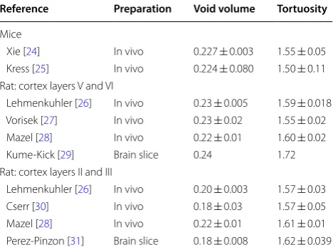
Table 1 Summary of ECS structural parameters determined by TMA-RTI experiments on neocortex of healthy, anesthetized adult rat and mice (layer indicated in table)
Uptake constant omitted from table because it has not been observed to vary much over in vivo rat brain experiments, 0.003–0.006 s−1 [20]
Reference Preparation Void volume Tortuosity
Mice
Xie [24] In vivo 0.227 ± 0.003 1.55 ± 0.05 Kress [25] In vivo 0.224 ± 0.080 1.50 ± 0.11 Rat: cortex layers V and VI
Lehmenkuhler [26] In vivo 0.23 ± 0.005 1.59 ± 0.018 Vorisek [27] In vivo 0.23 ± 0.02 1.55 ± 0.02 Mazel [28] In vivo 0.22 ± 0.01 1.60 ± 0.02 Kume-Kick [29] Brain slice 0.24 1.72 Rat: cortex layers II and III
where: Cmax = the peak concentration in the TMA
con-centration curve, Cmax,high rep = Cmax for the highest
experimental replicate, Cmax,low rep = Cmax for the lowest
experimental replicate.
Replicates reported by Cserr et al. in rats, Xie et al. in mice and raw data obtained by the authors for indi-vidual replicates in mice presented in Kress et al., reveal consistent variability in reproduced TMA concentration curves—the range is 70–90% [24, 25, 30]. Although these three experiments represent a fraction of all RTI data, such a consistent experimental range leads one to ques-tion whether some physical phenomenon is being over-looked that may be revealed by analyzing the data using models different from diffusion-only in a homogeneous material.
Integrative Optical Imaging (IOI) was developed to study the brain-transport properties of large molecules [32]. In the IOI method, macromolecules carrying a fluorescent label are injected by a pressure pulse and their progress measured by fluorescence microscopy. Although conceptually simple, analysis of the measure-ments is complex as the CCD camera registers a two-dimensional image of a three-two-dimensional “cloud” of diffusing molecules. Thus reported intensities do not correspond to actual concentrations, but some form of projection that depends on the optical characteristics of the imaging system. Analysis of the data to determine tortuosity applies the same model of diffusion-only trans-port in a homogeneous material (void volume cannot be
calculated by IOI, but is often assumed to be the same as for small molecules). Tortuosity generally increases with molecular size, however, molecular shape and flexibility also play a role. The majority of data is from brain slices. However, in vivo IOI became possible around 2006 and this body of data continues to grow. The success of the experimental techniques that rely upon a diffusion-only model (RTI and IOI) lends credence to the theory that bulk flow may not be important to molecular transport in the brain interstitium.
Microscopy is another tool used to study transport in the brain; it can be qualitative or semi-quantitative. In vivo injection of a tracer followed by ex vivo micro-scopic investigation of fixated tissue is a dependable, though coarse method. In a 1981 study, Cserr et al. injected radiolabeled tracers varying in size from 0.9 to 69 kDa into brain interstitium and measure their clear-ance rate over time. All molecules cleared at similar rates, supporting a convective-dominated model of transport [33]. Cserr noted the molecules followed “preferential routes”, possibly associated with vasculature. However, the experiments lacked the spatial resolution to resolve whether bulk flow was occurring throughout the brain interstitium or was restricted to the PVS.
More recently, Iliff et al. used in vivo two-photon laser scanning microscopy to follow clearance of different-sized tracers through the brain and reported indications of interstitial bulk flow [4]. Transport from the subarach-noid CSF down the periarterial space and into the brain interstitium was observed for three tracers of varying molecular size (3, 40, and 2000 kDa, the largest tracer did not enter the interstitium) moving at similar rates— Iliff interpreted the results as being caused by convective flow. Iliff et al. used ex vivo fixation to observe the trac-ers leaving the inttrac-erstitium along large venous structures to primary para-venous drainage pathways. In studies that confirmed the findings from Cserr et al., Iliff and colleagues observed the clearance rate of interstitially delivered Dextran-10 (10 kDa) was identical to mannitol (380 Da) [4]. Smith et al. conducted experiments similar to those of Iliff et al., corroborating convective transport along perivascular pathways, but finding that transport in the ECS was consistent with pure diffusion [5]. However, Mestre et al. [6] demonstrated the choice of anesthesia and tracer injection by pressure pulse employed by Smith et al. may suppress CSF influx, resulting in hindered tracer transport in the ECS. Smith et al.’s photo-bleaching results supporting diffusion-only in the interstitium were not questioned.
Iliff et al. also observed a 70% reduction in mannitol clearance from Aqp4 knockout (KO) mice compared to wild-type (WT) mice, hypothesizing that astroglial aqua-porin-4 (AQP4) may support interstitial and facilitated 0
0.2 0.4 0.6 0.8 1 1.2 1.4 1.6
0 50 100 150 200
TMA Concentration (mM)
Time (sec)
Source off
Source on
Fig. 2 TMA concentration curves for each replicate of young adult mice from Kress [25], generated from data for void volume, tortuosity, and uptake using RTI equations from Nicholson [14]. The replicates demonstrate experimental variability, where range is 88% and the standard deviation in Cmax is 36%. The inset shows an RTI
solute transport. Smith repeated these experiments, but did not observe differences in clearance for Aqp4 KO vs. WT mice. However, a recently published study con-curred that CSF influx is higher in WT mice than in four different Aqp4 KO lines; and demonstrated a significant decrease in tracer transport in KO mice and rats [6]. Fur-ther, the study established that anesthesia, age, and tracer delivery may explain the opposing results.
Estimating interstitial bulk‑flow
Diffusion is always occurring. Convection requires a driv-ing force, such as a pressure gradient, to generate bulk flow. It is hypothesized that a small pressure difference exists between the periarterial and perivenular space [4, 34], providing a mechanism for bulk flow across the interstitium. Bulk flow velocity in porous media can be calculated using Darcy’s law
v= −k′(∇P)
, where k′ is
hydraulic conductivity, ∇P is the pressure gradient and v is the superficial velocity. Table 3 reports literature val-ues for hydraulic conductivity in brain tissue, which range over two orders of magnitude. The pressure gradient is the difference in pressure between the periarterial and perivenular walls divided by the distance between them. This pressure gradient is unknown, but can be estimated. There are two schools of thought on the genesis of the pressure gradient: (1) hydrostatic pressure, originating from intracranial pressure of less than 10 mmHg peak-to-peak, and (2) hydrodynamic pressure, generated by arteriolar pulsation (65–100 mmHg maximum pressure) translating through the elastic vascular walls and bounded by the more rigid perivascular walls [34]. The hydrostatic pressure gradient in the brain is probably quite small, with an estimated upper limit of 1 mmHg mm−1 [35]. The hydrodynamic pressure gradient would be larger, but still much less than the arteriolar pressure. From the arteri-olar pressure, hydrodynamic pressure would be reduced (1) through translation across the vascular wall and (2) by flow of ISF through possible restrictions in the periarteri-olar wall (either aquaporin channels in the endfeet or gaps between endfeet). Therefore, at the periarteriolar wall just within the interstitium, the hydrodynamic pressure will be a small percentage of the arteriolar pressure and higher than the very low perivenular pressure.
Published simulations
Published simulations of transport in the brain fall into three categories: (1) structural or geometric models [20], (2) compartment models [36], and (3) continuum trans-port models. Transtrans-port models are derived using conser-vation principles. Many transport models for biological tissues successfully use the porous media assumption [37]. Both Jin et al. [38] and Holter et al. [35] developed thorough transport models of interstitial flow through
an extracellular matrix constructed based on the EM work of Kinney for the rat CA1 hippocampal neuropil [39]. Each adjusted the EM in different ways to increase the void volume of the ECS to match experimental val-ues of around 20% (volume changes are known to occur during tissue preparation and embedding for EM). Jin calculated a hydraulic conductivity of 1.2 × 10⁻⁶ cm2 mmHg−1 s−1 and Holter a hydraulic conductivity of 2 × 10⁻⁸ cm2 mmHg−1 s−1. Holter, using a hydrostatic pressure assumption, predicted average intrinsic veloci-ties of less than 1 μm min−1 (superficial velocities of less than 0.2 μm min−1). Jin’s model includes diffusion and convection of a solute, investigating pressure differences of 0–10 mmHg and concluding: (1) convection preferen-tially accelerates transport of large molecules, (2) pres-sure differences of > 1 mmHg are required for convection to augment transport, and (3) diffusion alone adequately accounts for experimental transport studies [38]. Jin et al. verified their model using visual comparisons to (1) Iliff’s two-photon microscopy data [4] and (2) Thorne’s IOI data [40] (both for 3-kD molecules). However, concen-trations predicted from their 2D model are not a direct comparison to intensity measured in an IOI experiment where the 2D image is convoluted by the projection from the 3D “cloud” of molecules (see IOI above). Asgari et al. show diffusion-only solute transport in the interstitium is increased by periarteriolar dispersion over periarteri-olar diffusion [15]; for an interstitial injection, dispersion results in a lower solute concentration at the PVW. Dif-ferent injection scenarios are investigated and demon-strate agreement with previously opposing experimental observations, providing hypotheses for both influx and efflux along either the periarteriolar or perivenular route. Asgari et al. also compared solute transport for 20-nm and 14-nm astrocytic endfeet gaps, with the smaller gap leading to a significant reduction in transport and corre-sponding increase in interstitial solute concentration.
The goal of this work is to present a model of trans-port in the brain interstitium that can be quantitatively compared with well-established experimental data, and can test current hypotheses of interest in brain trans-port. Although studies utilizing sophisticated microscopy or IOI may be more contemporary and offer details not elucidated by RTI (such as the movement of macromol-ecules), they do not provide sufficient (microscopy) or applicable (IOI) quantitative data with which to verify the model. This work focuses on RTI experiments, which provide a large body of reviewed and confirmed data, with significant and accessible quantitative substance. The model is used to investigate (1) the presence of bulk flow in the brain interstitium by applying diffusion-only and diffusion with convective bulk flow to transport-model simulations of RTI-TMA experiments, and (2) the effect of perivascular exchange on the same.
RTI experiments in the context of interstitial bulk flow Although RTI experiments originally relied upon a dif-fusion-only model, recent research findings encourage investigating the potential for bulk flow in the interstit-ium between periarterial and perivenous spaces. There-fore, let us perform a thought experiment with these in mind. In an RTI experiment, two probes are inserted into the brain approximately 150 μm apart (Fig. 2 insert). The first (source) probe delivers molecules to the brain tissue; the second (detection) probe measures the concentration of those molecules over time. In an isotropic, diffusion-only model, the concentration is symmetric in space—it is the same in any direction at a given distance from the source. In a convective flow field however, the concentra-tion would vary depending on the orientaconcentra-tion of the path from source to detection point relative to the flow field. If the solute is diffusing in the same direction as the con-vective flow, a molecule moving away from the detection probe would be carried away more rapidly by the bulk flow, resulting in less accumulation and a lower maxi-mum concentration. If the solute is diffusing against the convective flow, any solute randomly diffusing away from the detection probe would be carried back by bulk flow, resulting in greater accumulation and an overall increase in concentration. Since it is unlikely experimentally to align the probes with any potential flow field, there would most likely be a random sampling of orientations relative to the postulated flow field as each RTI test is performed, resulting in spread or range in the experimental data if bulk flow was present. As we will show using the model, larger bulk flows result in higher range and lower bulk flows or the absence of bulk flow results in lower range. Reciprocally, larger experimental range opens the poten-tial for higher bulk flows being theoretically possible,
and lower experimental range would imply a limit on the magnitude of any possible bulk flow.
Methods
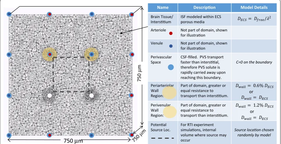
A finite-element model of transport in the brain inter-stitium was developed based on porous-media flow and mass-transport equations. The model domain is a three-dimensional section of the interstitium with penetrating vasculature (eight arterioles and eight venules, typically). Figure 3 shows a two-dimensional slice of the domain where shading illustrates the PVS and PVW and the table relates the physiology to aspects of the model. Several model domains were tested to determine the size and shape that minimized the effect of the exterior bounda-ries on the simulation results. The potentially slower mass transfer through the perivascular wall is modelled as a narrow region surrounding each vessel where the diffusivity is a percentage of interstitial diffusivity. The PVS becomes a boundary of the model domain, where exchange between the PVS and the interstitium is mod-eled through the application of boundary conditions to the vessel walls.
The ISF is assumed to be an incompressible Newtonian fluid, and the brain tissue is assumed to exhibit porous media flow behavior. The flow velocity is modeled using Darcy’s law:
combined with steady-state mass conservation:
where v is the superficial velocity, k′ is the hydraulic
con-ductivity, and P is the pressure. An oscillatory pressure is applied at the periarteriolar walls (different pressure magnitudes are explored and specified for each result), simulating physiological arteriolar pulsations. A pres-sure of zero is assumed at the perivenular walls. On the remaining exterior boundary, a symmetry assumption is used. Hydraulic conductivity is assumed to be homoge-neous and isotropic. The distance between penetrating vessels varies by vessel size and location within the brain, and also by species. Here we are interested in the aver-age distance between a distal penetrating arteriole and the nearest post-capillary venule in the rat neocortex. A value of 250 μm (center-to-center) is used based on limited anatomical data and values employed in similar models (see Table 2). To summarize results, the simu-lated superficial-velocity is averaged both in space and time; the spatial average is a volume-weighted average over the entire domain.
The mass transport equations modified for porous brain tissue are based on Nicholson and Phillips [14, 23]:
(1)
v= −k′(∇P)
(2)
∇ ·v=0
(3)
∂c ∂t =D
∗∇2
c+ s
where: c= concentration in the ISF, D∗
= apparent dif-fusivity = D/λ2, s= source term, α= void volume = VECS/ Vtotal, f(c)= uptake term, assumed to be zero for simu-lations performed here (TMA was chosen as a probe because it exhibits no cellular uptake).
A solute may exit through either the periarteriolar or perivenular walls. As transport in the PVS is known to be much faster than in the interstitium [4, 5], it is assumed that upon reaching the PVS a solute is rap-idly transported away. Note that no assumption about the direction of perivascular transport is required, only that it is rapid relative to interstitial transport. There-fore, a boundary condition of c=0 is used on the vessel walls (see Fig. 3). For the perivascular walls, both tight, as observed by Mathiisen [10], and loose, as observed by Korogod [13], arrangements were considered. For the tight PVW case, we estimate the diffusivity in the periar-teriolar wall as:
It is not computationally feasible to refine the mesh to resolve the 1.5 μm thickness of the endfeet, therefore
Dwall=DECS
0.3%of wall is endfeet gaps
20%void volume ECS
24 nmendfeet gaps
60 nmECS gaps =0.6%DECS
an equivalent mass-transfer resistance (L/D) is used—a higher diffusivity for a longer distance:
It has been proposed that the perivenular wall is “looser” with respect to the transport of solutes than the periarteriolar wall [38], so we choose D′arteriolar wall= 5% DESC and D′venular wall= 10% DESC. For the loose PVW case, D′wall=DECS . A no-flux boundary condition is applied to all other boundaries. Initial conditions differ depending on the physical situation being simulated and are given below. Apparent diffusivity is assumed to be homogeneous and isotropic.
In RTI experiments, a current is applied to the probe, creating a source of molecules at the probe’s insertion
point. The RTI probe is represented as a point source, an assumption that is consistent with previous analysis
D′wall=Dwall
12.5µmchosen wall thickness
1.5µmactual wall thickness
=5%DECS
for12.5µmwall thickness
750
µ
m
750
µ
m
Name Model Details
Brain Tissue/ ISF modeled within ECS porous media
Arteriole Not part of domain, shown
Venule Not part of domain, shown
Perivascular
Space CSF-filled. PVS transport therefore PVS solute is rapidly carried away upon reaching this boundary.
C=0 on the boundary
Periarteriolar Wall Region:
Part of domain, greater or equal resistance to
Perivenular Wall Region:
Part of domain, greater or equal resistance to
Source Loc. For RTI experiment volume where source may
occur randomly by model
riolar
:
lar
: or
or
Fig. 3 Finite-element domain illustrating physiology incorporated into model (2-dimensional slice of 3-dimensional domain). Cubic domain measures 750 μm on a side (0.4 mm3) with 8 penetrating arterioles and 8 penetrating venules. Red dots mark arterioles. Dark blue dots mark
of RTI data [14]. The source magnitude is derived from Faraday’s law: s=(I/F)·(M/z)·nt , where nt is an
experimentally measured probe efficiency. Concentration versus time is measured at a detection point 150 μm from the source. Experimental variability among replicates is of key interest in the present work. When executing an RTI experiment, the probes are inserted with very limited knowledge of neighboring arteriole and venule locations. Therefore, to simulate experimental variability, seven ran-dom source point locations are chosen within the center 195 µm × 195 µm × 195 µm of the domain. A solution is generated for each source point, and curves of concen-tration vs. time are recorded for 16 detection points sur-rounding each source point at a distance of 150 µm. The exterior boundaries have been placed far enough from the source to have little effect (this was tested by varying the domain size), so the no-flux boundary condition is sufficient. Initially, solute concentration is c=0 through-out the domain. TMA free (unhindered) diffusivity (D) is 1.3 × 10⁻⁵ cm2 s−1 [14]. For RTI experimental data used
for comparison to simulations, subjects were anesthe-tized, using urethane for Cserr experiments and keta-mine/xylazine for Xie and Kress.
The clearance simulation, which is symmetrical in the axial direction of the vessels, utilizes a two-dimen-sional model that looks exactly like the slice shown in Fig. 3. An initial uniform concentration of soluble Aβ is applied to the interstitium and its concentration tracked over time for various conditions. Aβ diffusivity is estimated based on the free diffusivity of Dextran 3, D = 2.3 × 10⁻⁶ cm2 s−1, with a tortuosity of 2.04 [20].
The resulting system of partial differential equations is solved using FEniCS [41, 42]. The time-derivative is discretized using a backward difference (i.e., an implicit method). The finite element meshes on which the com-putations are performed are generated using CGAL [43]. The bulk of the simulations were performed on a mesh consisting of over 880,000 tetrahedral elements. The accuracy of the results was tested by (1) decreasing the time step by half and, separately, (2) approximately
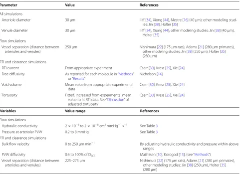
Table 2 Model parameters and variables
Parameters are held constant; they are either taken from literature or fitted from experimental data. Variables are varied to test different transport hypotheses (see Table 4)
Parameter Value References
All simulations
Arteriole diameter 30 μm Iliff [34], Xiong [44], Mestre [16] (40 μm); other modeling stud-ies: Jin [38], Holter [35]
Venule diameter 30 μm Iliff [34], Xiong [44]; other modeling studies: Jin [38] (40 μm), Holter [35]
Flow simulations
Vessel separation (distance between
arterioles and venules) 250 μm Nishimura [other modeling studies: Jin [22] (175 μm rats), Adams [38] (250 μm), Holter [21] (280 μm primates), 35] (280 μm)
RTI and clearance simulations
RTI current From appropriate experiment Cserr [30], Kress [25], Xie [24] Free diffusivity As reported for each molecule in “Methods”
or “Results” Nicholson [14] Void volume Mean value from appropriate experimental
data Cserr [30], Kress [25], Xie [24] Tortuosity Fitted. Increased from experimental mean
value to fit RTI data. See “Discussion” of adjusted tortuosity
Cserr [30], Kress [25], Xie [24]
Variables Value range References
Flow simulations
Hydraulic conductivity 2 × 10⁻⁶ to 2 × 10⁻⁸ cm2 mmHg−1 s−1 See Table 3
Pressure at arteriolar PVW 0.2 to 8 mmHg See Table 3
RTI and clearance simulations
Bulk flow velocity 0 to 250 μm min−1 By adjusting hydraulic conductivity and pressure within above
ranges
PVW diffusivity 0.6 to 100% of DECS Mathiisen [10], Korogod [13], (see “Methods”)
Vessel separation (distance between
doubling the number of mesh elements; each resulted in less than a 1% variance. Post-processing of simulation data is carried out using Excel and Paraview.
Model parameters and variables
Parameters and variables used in the model along with their values, or value range, and references are reported in Table 2. Many previous models of transport in the brain required a number of assumptions to obtain a sim-ple enough model that an analytical solution is available. We have purposefully sought to minimize the number of assumptions and adjustable variables to examine a spe-cific hypothesis, bulk flow. For the model presented in this paper, some assumptions are more likely to be cor-rect than others. For example, the values used for free diffusivity, void volume, and distance between vessels are all based on extensive experimental measurements and are likely to be relatively accurate. For variables like these where we are confident in the assumptions made, we use the values given in Table 2 and those values are not varied significantly in the analysis of the model predic-tions. For other variables, notably the pressure difference between the periarteriolar wall and the perivenular wall, there is far more uncertainty so a large range of values is explored, and then model predictions are compared to experimental measurements.
Results
Interstitial bulk‑flow simulations
Bulk-flow simulations were performed for a range of pressures, assuming both the hydrostatic and hydro-dynamic cases (see “Background”), and the range of
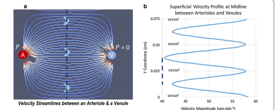
hydraulic conductivities found in the literature. For the hydrostatic case, a pressure of 0.2 mmHg is used. A maxi-mum hydrodynamic pressure difference of 1–10 mmHg is used (the same range is explored by Jin [38]), based on 1–10% of systolic arteriolar pressure, which is approxi-mately 65–100 mmHg. The resulting bulk-flow velocity varies with space and time; Fig. 4 shows example veloc-ity streamlines between an arteriole and a venule and an instantaneous velocity profile across the midline slice of the domain. Velocity is highest in a direct line between arteriole and venule, but only varies ± 18% from the aver-age. Table 3 reports the average bulk-flow superficial-velocity calculated from flow simulations for the range of hydraulic conductivities and pressures. To readily compare different conditions, the velocity is averaged over time and the entire domain. A bulk flow superfi-cial-velocity of 0.5–25 μm min−1 (0.1–4 × 10⁻⁴ cm s−1) results from mid-range hydraulic conductivity and the range of pressures. This corresponds to a superficial volu-metric flow rate of 0.05–2.4 μL g−1 min−1 (for brain tis-sue density = 1.0425 g cm−3).
Simulations of real‑time iontophoresis experiments
Comparison of simulations to RTI experimental data is used to test theories for mechanisms of interstitial trans-port in the brain: diffusion, convection, perivascular exchange, and conditions at the perivascular wall. In addi-tion, the sensitivity of results to sources of experimental variability, vessel separation, and velocity magnitude are investigated. A list of transport simulations performed and a summary statistical analysis comparing the simula-tions to the experimental values is given in Tables 4 and 5.
Velocity Streamlines between an Arteriole & a Venule
A
V
= 0
vessel
vessel
vessel
vessel
a b
Fig. 4 Superficial velocity streamlines and velocity profile for v= 50 μm min−1. a Streamlines show how flow is organized from the arteriole to
As discussed in the introduction, many sources of variability are inherent to RTI experiments. We begin by attempting to quantify some of these sources of
variability, namely inter-animal variation, tissue hetero-geneity, and probe separation; others, such as tissue dam-age and the physiological state of the animal under study, are difficult to estimate. The tissue is simplistically char-acterized by α and λ, therefore the sensitivity of the sim-ulation results to changes in these values was explored. Void volume between different experimental studies varies by at most 0.01 for the same general layer of the cortex, and tortuosity by 0.05 (Table 1). Table 4 reports this maximum variability due to tissue variation to have a combined range of 0.21. An error in probe separation measurement of 2 μm, results in a range of 0.02. Since diffusion-only simulations result in a range of zero, the same concentration curve in all directions independent of source location, the base case of diffusion-only plus the estimate of experimental variability is 0.23—about one-third of the observed experimental range.
Table 3 Simulation results for bulk-flow superficial-velocity in the brain interstitium
Volume-averaged (over full domain), time-averaged velocity is reported for each condition. A range of hydraulic conductivity values from the literature are reported and used in the simulation. A range of periarteriolar wall pressures are used, and further described in the text. Wall pressure is an oscillatory function in the model; maximum and mean pressure are reported in the table
a Reports value of 1.2 × 10⁻⁶ cm2 mmHg−1 s−1, for parenchyma only based on simulation Hydraulic conductivity (cm2
mmHg−1 s−1) Average bulk‑flow superficial‑velocity (μm min −1)
For
Pavg= 0.2 mmHg
For
Pmax= 1 mmHg
Pavg= 0.8 mmHg
For
Pmax= 3 mmHg
Pavg= 2.4 mmHg
For
Pmax= 10 mmHg
Pavg= 8 mmHg
2 × 10⁻⁶ [38, 45]a 5 25 75 250
2 × 10⁻⁷ [46] 0.5 2.5 7.5 25
2 × 10⁻⁸ [35] 0.05 0.25 0.75 2.5
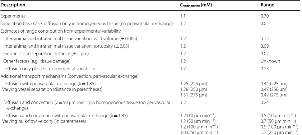
Table 4 Summary of simulations and sensitivity analysis performed
Using Cserr et al. [30] experimental case and base simulation conditions of α = 0.18, λ = 1.6, diffusion only in homogeneous tissue (no perivascular exchange routes). Simulations with perivascular exchange use λ = 1.85 for reasons described below
Description Cmax,mean (mM) Range
Experimental 1.1 0.70
Simulation base case: diffusion only in homogeneous tissue (no perivascular exchange) 1.2 0.0 Estimates of range contribution from experimental variability
Inter-animal and intra-animal tissue variation: void volume (± 0.005) 1.2 0.12 Inter-animal and intra-animal tissue variation: tortuosity (± 0.05) 1.2 0.09 Error in probe separation distance (± 2 μm) 1.2 0.02 Other factors (e.g., tissue damage) 1.2 Unknown Diffusion only plus est. experimental variability 1.2 0.23 Additional transport mechanisms (convection, perivascular exchange)
Diffusion with perivascular exchange (λ = 1.85)
Varying vessel separation (distance in parentheses) 1.25 (225 μm)1.28 (250 μm) 1.31 (275 μm)
0.44 (225 μm) 0.47 (250 μm) 0.42 (275 μm) Diffusion and convection ( v= 50 μm min−1) in homogeneous tissue (no perivascular
exchange) 1.2 0.24
Diffusion and convection with perivascular exchange (λ = 1.85)
Varying bulk-flow velocity (in parentheses) 1.2 (10 μm min
−1)
1.2 (50 μm min−1)
1.2 (100 μm min−1)
1.0 (250 μm min−1)
0.5 (10 μm min−1)
0.7 (50 μm min−1)
0.9 (100 μm min−1)
1.7 (250 μm min−1)
Table 5 Summary of boundary condition sensitivity analysis
For boundary condition sensitivity, base case is diffusion and convection ( v= 50 μm min−1) with perivascular exchange using vessel separation = 250 μm
Description Cmax,mean (mM) Range
Experimental 1.1 0.70 Boundary conditions
Tight perivascular walls ( Dwall=5%DECS) 1.2 0.66
Loose perivascular walls ( Dwall=DECS) 0.86 1.17
Loose perivascular walls, no flux condition on arterioles ( Dwall=DECS)
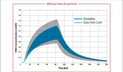
Diffusion only with perivascular exchange was simu-lated over a range of vessel separation (225–275 μm). Discrete locations where solute molecules leave the interstitium, at the PVW of the vessels penetrating the domain, contributes significantly to range by adding het-erogeneity to the tissue. Perivascular exchange results in a range of 0.42–0.47 depending on vessel separation (Table 4), equivalent to about two-thirds of the range observed experimentally. Cmax, mean increases with vessel separation, but no correlation is observed between ves-sel separation and range. The variability in range with vessel separation is likely due to small changes in the proximity between detection points and vessel locations. Figure 5 shows the range in concentration curves for a simulation with diffusion only and perivascular exchange (blue) compared to experimental data from Cserr (grey). The simulation results agree well in magnitude and shape with concentration curves from TMA-RTI experi-ments, but the range does not span the full experimental variability.
Diffusion and convection simulations were per-formed for a range of bulk-flow velocity, with and with-out perivascular exchange. Convection of 50 μm min−1
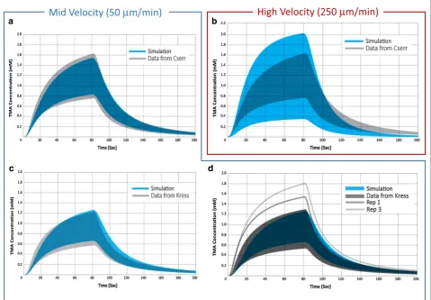
without perivascular exchange gives a range of 0.24. When perivascular exchange is included in the simula-tion, the range increases to 0.7. In Fig. 6a, the range of concentration curves for simulations performed with an average bulk velocity of 50 μm min−1 and perivascular exchange (blue) is compared to the range in Cserr’s data (grey). Simulations performed for various source-detec-tion path orientasource-detec-tions (see “Methods”) relative to the flow field reflect the dependence of concentration curve upon orientation with the flow field, and result in significant range across simulation replicates. The range generated by a convective superficial velocity of 50 μm min−1 com-bined with diffusion and perivascular exchange is equiva-lent to the full experimental range reported by Cserr.
Figure 6b shows the range of simulated concentration curves for an average bulk flow velocity of 250 μm min−1 (blue) compared with Cserr’s data (grey, same as Figs. 5, 6a). At flow rates of 250 μm min−1 and above, the range is extremely high, and does not agree with reported experi-mental observations.
Similar results are observed when we analyze the data from Kress et al. [25] for male and female healthy, young adult mice. Simulation results for diffusion-only and
Diffusion Only (0 µm/min)
Fig. 5 Range in TMA concentration versus time curves for experimental data compared with diffusion-only with perivascular exchange simulations. Experimental data from Cserr reported in grey (n = 33) [30] compared to diffusion-only simulations reported in blue (n = 112). Experimental median values were α = 0.18, and λ = 1.6. For simulation, v= 0 μm min−1, α = 0.18, and λ = 1.85, vessel separation = 250 μm. Variability in the simulation
a high bulk-flow velocity of 250 μm min−1, both with perivascular exchange, differ from experimental variabil-ity observations, similar to the Cserr data. In Fig. 6c, d, the range of concentration curves for simulations per-formed with an average bulk velocity of 50 μm min−1 (blue) is compared to the range in the Kress data (grey). Again, the range calculated from the simulation results accounts for the full variability in the experimental data for the female population. The two highest replicates from the male experimental data lie outside the range predicted by simulation. These high experimental repli-cates may have suffered from other sources of variability.
In the introduction, conflicting EM results regarding “tight” or “loose” endfoot arrangements at the perivas-cular wall were discussed. For the simulation results presented preceding this paragraph, a tight model was used, with the perivascular wall presenting a resistance to mass transfer greater than the ECS (see “Methods”). Simulations were also performed for a loose perivascu-lar wall where Dwall=DECS—the resulting
concentra-tion curves have a significantly lower Cmax,mean = 0.86
and much greater range = 1.17 than the experimen-tal data, Cmax,mean = 1.1 and range = 0.7 (Table 5). If
the boundary condition is further changed such that
a b
c d
Mid Velocity (50
µ
m/min)
High Velocity (250
µ
m/min)
Fig. 6 Range in TMA concentration curves for experimental data compared with diffusion and convection simulations with perivascular exchange. Simulations performed at a mid (50 μm min−1) and high (250 μm min−1) velocity based on bulk flow estimates. a Experimental data in rats from
Cserr et al. (grey, n = 33) [30] compared with diffusion and mid-velocity convection simulations (blue, n = 112). Experimental median values were α = 0.18, and λ = 1.6, assuming diffusion only. For simulation, v= 50 μm min−1, α = 0.18, and λ = 1.85. b Experimental data from Cserr et al. (grey,
n = 33) [30] compared with diffusion and high-velocity convection simulations (blue, n = 112). For simulation, v= 250 μm min−1. c Experimental
data in mice from Kress et al. (grey) for female (n = 9) [25] compared with mid-velocity simulations (blue). Experimental median values were α = 0.224, and λ = 1.6, assuming diffusion only. For simulations, average bulk flow velocity = 50 μm min−1, α = 0.224, and λ = 1.85. d Experimental
data in mice from Kress et al. (grey) for male (n = 11) [25] compared with mid-velocity simulations (blue). Experimental and simulation parameters same as c. The range for 50 μm min−1 simulation results is equivalent to the full variability reported by both Cserr et al. and Kress et al. consistent
with the presence of bulk flow. Range for the 250 μm min−1 simulation is much higher than experimental observations, suggesting that bulk flow in
material is only permitted to leave through the venu-lar PVW (no exchange through the arteriovenu-lar PVW), then there is better agreement with the experiment,
Cmax,mean = 1.2 and range = 0.75 for the simulation
(Table 4). One would expect similar results if the ves-sels were further apart and both exchange routes were available.
Is it possible that flow is induced by the RTI ment, and not physiological? Although the RTI experi-ment is designed to avoid electro-osmosis, it is possible that some occurs. Electro-osmosis means that instead of only TMA cations entering the brain tissue, solvent from the micropipette solution enters as well, generating a bulk flow. To understand the upper limit of the effect of electro-osmosis, a worst-case calculation was made assuming all of the TMA was delivered as the micropi-pette solution instead of as TMA cations alone. This worst case induced a bulk flow of only 0.6 μm min−1 at a distance of 150 μm from the source, a small fraction of the velocities discussed here.
The best agreement between simulations and experi-mental data results from a simulation tortuosity of 1.85, which is greater than the typical experimentally obtained value of 1.6. A higher tortuosity (λ) means a lower apparent diffusivity ( D∗ ), as D∗=D/2
. In tra-ditional RTI analysis, which assumes diffusion only, all transport mechanisms are lumped into this single variable, the apparent diffusivity. By overlooking other phenomena effecting transport—losses to perivascu-lar exchange and convection—transport rates of all mechanisms are essentially combined into the sin-gle apparent diffusivity, increasing its magnitude and decreasing λ. In contrast, the simulation distinctly separates both convection and losses through perivas-cular spaces from diffusive transport in the interstitial tissue. This separation of mechanisms in the simulation means the apparent diffusivity now represents only the diffusional transport and it is therefore lower relative to diffusion-only RTI analysis. This was confirmed by per-forming simulations in a homogenous material, with no perivascular exchange, for which the best fit for the data was given by the experimental value for tortuosity (usually λ = 1.6).
It was shown above that a bulk flow velocity of v= 50 μm min−1, with perivascular exchange, gives a range corresponding to the full experimental variability. However, if other sources of experimental variability are included, such as inter-animal tissue variation, a lower velocity would give better agreement. Therefore, for the following sections, we use a superficial bulk-flow veloc-ity of v= 15 μm min−1 to represent a more conservative estimate of v considering contributions from the other sources of experimental variability.
Implications for large‑molecule transport
TMA is a small molecule (114 Da) with a relatively fast diffusivity. Molecules of interest in brain transport, such as Aβ (4.5 kDa) and tau (45 kDa), which are thought to play a significant role in neurodegenerative pathologies, are larger and have slower diffusivities. The Péclet num-ber ( Pe ) is a ratio of convective to diffusive transport
rates:
Pe allows comparison of the relative importance of
con-vection to diffusion for molecules with different apparent diffusivities. If transport is predominantly diffusion, then
Pe≪1 , and if transport is primarily bulk flow, Pe≫1 .
For interstitial transport, solutes move through three “materials” with differing diffusivities: periarteriolar wall, brain interstitium, and perivenular wall. To account for all materials, a mass-transfer resistance in series model is used where:
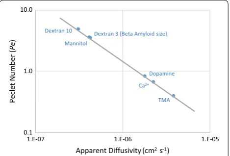
Figure 7 reports Péclet numbers for molecules relevant to brain transport as a function of their apparent diffusiv-ity for a bulk flow of v= 15 μm min−1. Tortuosity for the molecules other than TMA were measured by IOI [20] or radiotracer techniques [14] and adjusted for the tortuos-ity used here for the brain interstitium only.
Peclet Number(Pe)= rate of convection rate of diffusion =
Lv D
L
D(overall)=
L
D =
Lart.wallD art.wall
+LECS
DECS+Lven.wall
Dven.wall
0.1 1.0 10.0
1.E-07 1.E-06 1.E-05
Peclet Number
(Pe
)
Apparent Diffusivity (cm2s-1) Dextran 3 (Beta Amyloid size) Dextran 10
TMA Dopamine Mannitol
Ca2+
Fig. 7 Péclet number versus apparent diffusivity for various molecules of interest in brain transport. L = 250 μm, v= 15 μm min−1,
and apparent diffusivity (D*) specific to each molecule. Pe=v L/D* is
the ratio of convective to diffusive transport rates. For Pe≈1 , diffusive
and convective rates are balanced; for Pe>1 , convection exceeds
diffusion. The graph shows for v= 15 μm min−1 bulk flow is not large
As expected, TMA has a Péclet number less than 1 ( Pe≈0.4 ), indicating its interstitial transport is
diffu-sion-dominant. Therefore, TMA is an appropriate mol-ecule for probing the structure of brain tissue using a diffusive-transport assumption. However, Dextran-3 kDa (Dex3), similar in size to Aβ, has a Péclet number of 4, meaning convection will have an effect similar in magni-tude to, or potentially greater than, diffusion within the brain tissue. Many molecules of interest to brain patholo-gies are even larger than Dex3, therefore, the magnitude of convective transport due to bulk flow is likely to be of similar or greater magnitude than diffusive transport. It follows that bulk flow should be considered when study-ing large-molecule transport in the brain.
Clearance simulations
The previous discussion focused on the transport ties of brain tissue. Now we explore how these proper-ties impact the efficiency of clearing materials from brain tissue. Using the findings of previous sections, simula-tions of Aβ clearance were performed to investigate the impact of possible convective bulk flow on metabolite clearance. Iliff et al. report data for clearance of an inter-stitial injection of radiolabeled Aβ from the entire brain
for aquaporin-4 (Aqp4) null and WT mice [4] (AQP4 is a water transport channel localized to the astrocyte end-feet, Fig. 1). As the model presented here is of a small volume of the interstitium and it will be compared to data taken for the whole brain, an assumption is being made that transport through the interstitium is the rate-limiting step in molecular clearance. This is not known to be true, however, the interstitium does represent the smallest spaces in which extracellular transport is occur-ring. Calculations made using this assumption will result in a conservative assessment of transport rate through the interstitium as several processes are being ignored. None-the-less it seems an instructive exercise for testing our outcomes.
Assuming the absence of bulk flow in the Aqp4 null mice, a diffusion-only simulation (Fig. 8) predicts perivascular wall diffusivities of D′
arteriolar wall= 2.5% DESC
and D′
venular wall= 5% DESC—half those used above for
TMA. It is reasonable to expect higher tortuosity for a larger molecule within the tight perivascular walls. Using these wall diffusivities, simulations were performed for various interstitial pressure differences resulting in vari-ous bulk-flow velocities. A simulation for v= 7 μm min−1 shows best agreement with experimental data for the
0 0.1 0.2 0.3 0.4 0.5 0.6 0.7 0.8 0.9 1
0 5 10 15 20 25 30 35
Normailized Beta Amyloid Concentraon (C/
C0
)
Time (min)
Diffusion Only v=7 um/min v=15 um/min v= 50 um/min Experiment WT Experiment Aqp4
-/-Fig. 8 Aβ clearance from interstitial injection, experimental data compared with simulations. Experimental data from Iliff for Aqp4 KO and WT mice [4]. Simulation results at various bulk-flow rates and for diffusion only. Details of simulation described in “Methods”. Periarteriolar wall and perivenular wall diffusivities are 2.5% and 5% of interstitial diffusivity respectively, to fit experimental data for Aqp4 null mice (which are hypothesized to have no bulk flow in the interstitium). Based on conservative assumptions, simulations for a bulk-flow velocity of 7 μm min−1 fit the experimental data for
WT mice (Fig. 8). It should be noted that a bulk-flow rate of zero in the Aqp4 null mice is unlikely to be true as water transport also occurs through gaps in astrocytic endfeet; therefore, the fit presents a conservative calcu-lation of bulk-flow velocity, and higher bulk-flow veloci-ties are possible. Further, simulations show bulk flow to have a significant impact on clearance of Aβ, even at low velocities (Fig. 8).
Discussion
This work compares the range in simulated TMA-RTI concentration curves inherent to different transport mechanisms to experimental range to show evidence of (1) interstitial convective flow and (2) perivascu-lar exchange. Experimental range will be comprised of contributions from several sources, which are likely to interact in ways that are not purely additive. However, identifiable sources were investigated separately in an attempt to quantify their relative contributions. The sim-plest case of diffusion only in a homogeneous medium has no variability with source or detection points, and therefore results in a range of zero. The contribution of tissue variation between experimental subjects and within an individual subject to range was estimated based on differences in void volume and tortuosity between experimental data sets and found to be 0.23 (about one-third of the full experimental variability of 0.70). Addi-tional sources of experimental variability, such as tissue damage, are also potentially present but not possible to quantify. This leaves us with approximately two-thirds of the full experimental variability that may be caused by transport mechanisms not included in the experimental data analysis.
Simulations attribute a relative range of 0.42–0.47 to diffusion and perivascular exchange for vessel separation ranging from 225 to 275 μm. The boundary-condition assumption of a zero solute concentration in the perivas-cular space is likely extreme. Asgari predicts perivasperivas-cular concentrations of about 30% of the tissue concentration approximately 20 min following interstitial injection [15], for a model assuming dispersive transport in the perivascular space. A model assuming perivascular con-vection may predict lower perivascular concentrations, but likely not zero. A more realistic perivascular con-centration would result in a lower range attributable to perivascular exchange. In addition, range due to perivas-cular exchange is likely to be dependent on the arrange-ment of the arterioles and venules, which were not varied in this work, making higher or lower range contributions possible.
Simulations also show that the presence of convection can contribute significantly to range, depending on the magnitude of the bulk-flow velocity, with a contribution
of 0.24 at v= 50 μm min−1. When all transport mecha-nisms are combined, and quantifiable experimental vari-ability sources are added, the resulting range matches the experimental variability for v= 10–50 μm min−1. Simi-lar interstitial bulk-flow superficial velocities have been reported in the literature: Abbott et al. estimated 10 μm min−1 in the cuttlefish brain [47]; Rosenberg et al. meas-ured 10.5 μm min−1 in white matter [48]; however, Holter et al. calculate a much lower bulk flow velocity around 0.3 μm min−1 [35]. The shape of the simulated concentration curves for the combination of all transport mechanisms also agrees well with the experimental curves, although simulated curves deviate from experimental-fit curves over the first 5 s of the RTI experiment. Understand-ing this difference may help identify relevant transport mechanisms not accounted for currently. Even though it is difficult to say the exact proportions of sources and mechanisms that comprise the full experimental range, at a minimum it has been demonstrated based on this anal-ysis of RTI data that the presence of bulk flow cannot be excluded.
Simulations of Aβ clearance calculate a conservative bulk flow velocity v= 7 μm min−1. This estimate includes the conservative assumptions of no ISF flow in Aqp4 KO mice and transport across the ECS as the only step in the complex process of transport through the entire brain; and may therefore be considered a lower limit for bulk-flow velocity. Smith et al. found no difference in clearance between WT and Aqp4 KO mice. However, Mestre et al. demonstrated the choice of anesthesia and meth-ods of tracer injection employed by Smith suppress CSF influx [6]. Mestre’s work includes a meta-analysis citing decreased ISF tracer clearance in Aqp4 KO mice and rats in five of six studies (the one outlier being Smith et al.).
specifically considered in the model, except to the extent that a reduction in pressure across the wall is taken into consideration when estimating a reasonable pressure range to explore.
It may be possible to further investigate the presence or absence of interstitial convection through comparison to experiments where any potential physiological flow has ceased. Physiological flow is ceased in brain slice experi-ments, where reported tortuosity is higher than in vivo experiments for the same region of the brain (Table 1) indicating slower transport than with physiological flow present. Brain slice experimental-replicate data present an opportunity that could be pursued in the future. How-ever, brain slice experiments pose additional sources of variability not present during in vivo experiments, e.g., water uptake during incubation and loss of TMA from the slice surface that is not accounted for by conventional analysis [29]. The additional sources of variability would need to be quantified for a useful comparison.
Comparison of simulation to experimental range sup-ports the possibility of interstitial bulk-flow velocity on the order of 10 μm min−1–an outcome independent of the origin of said flow. Based on an intermediate value for hydraulic conductivity, such a flow rate requires an average pressure difference of around 2–5 mmHg. These findings are consistent with Jin [38], who reported “sig-nificant convective transport requires a sustained pres-sure difference of several mmHg”. A 2–5 mmHg prespres-sure magnitude requires hydrodynamic pressure, but leaves outstanding the question of how much of the arteriolar pressure wave (with a peak pressure between 65 and 100 mmHg) is translated beyond the vessel wall. Pressure generated in the periarterial space by arteriolar pulsation is a hypothesis for which there is conflicting support [15, 16, 34]. However, as long as the vessel wall is not com-pletely rigid, a small fraction will be translated and the exact amount of this translation is thus an important area of further investigation.
The interstitial bulk-flow velocity v= 10 μm min−1 can also be expressed as a volumetric flow rate of 1.0 μL g−1 min−1. Hladky’s impressive review of clearance of spe-cific substances from the brain interstitium calculates a perivascular flow rate of 0.6–1.2 μL g−1 min−1 based on observations of inulin and sucrose clearance from brain tissue [7] (although Hladky notes the calculated perivas-cular rate exceeds current estimates of CSF production rate, 0.25 μL g−1 min−1, and is unlikely to be made up by fluid secretion from the BBB). If the link between periar-terial and perivenular flow is bulk flow across the inter-stitium, then the interstitial flow rate would also have to be around 1 μL g−1 min−1 due to continuity of mass— consistent with conclusions from the work presented here.
Transport conditions at the perivascular wall were investigated, with the best fit resulting from a tight wall assumption, based on Mathiisen [10]. In the simulation where perivascular wall diffusivity did not differ from ECS diffusivity, based on Korogod [13], less TMA accu-mulation due to faster transport at the PVW resulted in low Cmax,mean= 0.86 mM and a large range = 1.17,
compared to the experiment Cmax,mean= 1.1 mM and
range = 0.7. Thus simulations support a mass-transfer resistance at the PVW, and further work is necessary to clarify the details of the PVW resistance.
This work focused on RTI experimental data due to its quantitative nature and accessibility; additional informa-tion may be gleaned by investigating IOI and magnetic resonance imaging (MRI). Although IOI experimental data is complex to analyze and not directly comparable to simulation (as described in “Background”), compari-son of concentration simulations to intensity measure-ments may still provide useful insights into mechanisms of transport, particularly for larger molecules. MRI, which enables studies of the entire brain, is a promising field, especially as image resolution improves (MRI can currently resolve in the sub-millimeter range; resolution of microns is required to measure interstitial bulk flow). Contrast-enhanced MRI data following the transport of tracers from the cisterna manga into brain interstitium has been reported in rats [49, 50]. MRI images have the additional benefit of also containing key anatomical fea-tures, which may provide accurate and specific informa-tion such as vascular arrangement and dimensions that are currently estimated (Additional file 1).
Conclusions
In conclusion, the analysis described here, comparing transport simulations to previously published experi-mental data, supports that interstitial transport may occur by both diffusion and convection (bulk flow), with both mechanisms potentially relevant and the appar-ent diffusivity, related to molecular size, determining which is dominant. Simulations show that published RTI experimental range and tracer clearance studies allow for interstitial bulk-flow superficial velocities from v= 7 to 50 μm min−1; corresponding to intrinsic velocities on the order of 100 μm min−1 ( v
i=v/0.2) . A useful finding for
the scientists developing approaches for evaluating slow interstitial bulk flow over long distances. Results also support (1) the hypothesis of perivascular space allow-ing exchange between the brain interstitium, the suba-rachnoid CSF, and perivenous drainage out of the brain; and (2) increased mass transfer resistance at the PVW (as compared to the ECS).

![Fig. 2 TMA concentration curves for each replicate of young adult mice from Kress [tortuosity, and uptake using RTI equations from Nicholson [replicates demonstrate experimental variability, where range is 88% and the standard deviation in 25], generated f](https://thumb-us.123doks.com/thumbv2/123dok_us/214175.1514877/4.595.57.292.87.242/concentration-replicate-tortuosity-nicholson-replicates-demonstrate-experimental-variability.webp)