The problem of the second wind turbine – a note on a common but ﬂawed wind power estimation method

(1)

www.earth-syst-dynam.net/3/79/2012/ doi:10.5194/esd-3-79-2012

Earth System

Dynamics

The problem of the second wind turbine – a note on a common but

flawed wind power estimation method

F. Gans, L. M. Miller, and A. Kleidon

Biospheric Theory and Modeling Group, Max Planck Institute for Biogeochemistry, Hans-Knoell-Strasse 10, 07745 Jena, Germany

Correspondence to: F. Gans ([email protected])

Received: 29 April 2010 – Published in Earth Syst. Dynam. Discuss.: 8 June 2010 Revised: 19 March 2012 – Accepted: 11 May 2012 – Published: 8 June 2012

Abstract. Several recent wind power estimates suggest that

this renewable energy resource can meet all of the current and future global energy demand with little impact on the atmosphere. These estimates are calculated using observed wind speeds in combination with specifications of wind tur-bine size and density to quantify the extractable wind power. However, this approach neglects the effects of momentum extraction by the turbines on the atmospheric flow that would have effects outside the turbine wake. Here we show with a simple momentum balance model of the atmospheric bound-ary layer that this common methodology to derive wind power potentials requires unrealistically high increases in the generation of kinetic energy by the atmosphere. This in-crease by an order of magnitude is needed to ensure mo-mentum conservation in the atmospheric boundary layer. In the context of this simple model, we then compare the ef-fect of three different assumptions regarding the boundary conditions at the top of the boundary layer, with prescribed hub height velocity, momentum transport, or kinetic energy transfer into the boundary layer. We then use simulations with an atmospheric general circulation model that explic-itly simulate generation of kinetic energy with momentum conservation. These simulations show that the assumption of prescribed momentum import into the atmospheric boundary layer yields the most realistic behavior of the simple model, while the assumption of prescribed hub height velocity can clearly be disregarded. We also show that the assumptions yield similar estimates for extracted wind power when less than 10 % of the kinetic energy flux in the boundary layer is extracted by the turbines. We conclude that the common method significantly overestimates wind power potentials by an order of magnitude in the limit of high wind power

ex-traction. Ultimately, environmental constraints set the upper limit on wind power potential at larger scales rather than de-tailed engineering specifications of wind turbine design and placement.

1 Introduction

Several recent studies have quantified large-scale or global wind power availability by extrapolating kinetic energy avail-ability from measured wind speeds (Archer and Jacobson, 2005; Sta. Maria and Jacobson, 2009; Lu et al., 2009; Liu et al., 2008; Leithead, 2007).

Although the exact methodologies may differ, these stud-ies use a similar procedure. Hereafter, we will collec-tively refer to these studies as the “common method”. This methodology can be generally described as follows:

1. Observations of wind velocities, v, are derived for a large spatial area from a collection of surface stations (e.g. Archer and Jacobson, 2005), satellite measure-ments (e.g. Liu et al., 2008), or reanalysis data (e.g. Lu et al., 2009).

2. Technical specifications for a turbine are then used to specify the rotor height, rotor-swept area, and velocity dependent power characteristics.

(2)

4. The area is then populated with wind turbines at a den-sity limited by engineering constraints related to turbine wake turbulence, under the basic assumption that wind turbines do not influence the wind field outside their specific influential wake volume (e.g. Sta. Maria and Jacobson, 2009).

These studies collectively result in high wind power avail-abilities and exclude effects on larger scale atmospheric flow, since they assume kinetic energy consumption is limited to the turbine wake, but does not affect the large-scale flow.

In stark contrast, studies by Keith et al. (2004) and Wang and Prinn (2010) use global climate models which include consumptive effects and induced feedbacks from large-scale wind power extraction. These two studies also show signifi-cant climatic impacts of wind power removal on the climate system. Additionally, Miller et al. (2011) included these con-sumptive effects and estimated the maximum global land-based wind power availability from the atmospheric bound-ary layer (ABL) to be 18–68 TW, which is much lower than previous estimates and unavoidably associated with significant climatic differences.

The discrepancy in results between the two different methodologies is significant and must be resolved. Advo-cates of the common method usually argue that imprecisions in general circulation models (GCMs) and the associated rep-resentation of wind turbines therein cause the differences in climatic effects, and therefore the results should be disre-garded (e.g. see open discussion on Miller et al., 2011). In our opinion the assumption of an unaltered wind velocity out-side the turbine wake is the main reason for this difference, because it neglects the effects of turbine-related momentum removal from the atmospheric boundary layer.

The aim of this paper is to investigate the effect of not ac-counting for kinetic energy and momentum removal from the atmospheric flow during wind power extraction on different magnitudes of power extraction.

We will present a simple model which is based on the bal-ance of momentum and kinetic energy fluxes in the atmo-spheric boundary layer. We then compare the results of this simple model with the GCM simulation results of Miller et al. (2011).

2 Momentum and kinetic energy extraction from the atmospheric boundary layer

Wind turbines generate electrical power by removing kinetic energy from the atmospheric flow. The instantaneous rate of kinetic energy extraction from a moving fluid can be ex-pressed as

P =F ·v (1)

wherevis the velocity of the fluid, and the forceF is the rate of momentum extraction from the flow. Wind power is

there-fore proportional to the extracted momentum and the velocity at which this momentum is extracted. In general, the highest potential of extracting wind power is realized when there is a high velocity as well as a continuous source of momentum that can be utilized.

Equation (1) forms the basis for deriving the wind power formula used in the common methodology. The momentum density of a fluid moving at a velocity isρ v. The momen-tum flowing through the cross-section of a single turbine equals the momentum density multiplied by the flow ve-locity, Jp=ρ v·v, where Jp is the horizontal momentum

transport in the fluid. The assumption that the drag from turbines, Fturbine, is proportional to Jp (i.e. Fturbine∝ρ v2)

leads to the commonly known wind power extraction equa-tionPex∝A ρ v3, whereAis the wind-swept area of the wind turbine blades.

This equation is likely to give the impression that wind power availability is determined by measured velocities and air densities only, but its derivation shows that the flux of momentum is equally important. Wind turbines depend on the extraction of momentum, and in the absence of a con-tinual source of momentum, wind turbines would eventually stop the air from moving. In order to quantify the large-scale extractability of wind energy, it is therefore essential to quantify and model the sources of momentum and kinetic energy, thereby investigating their influence on wind power extractability.

We next consider the case in which we account for the momentum balance of the fluid from which kinetic energy is extracted. In the limit case of a completely developed wind farm, where all the surface area is equally covered with equidistant wind turbines, lateral sources of momentum can be neglected and only vertical fluxes of momentum add to the overall momentum balance of the system. In the absence of external forces, momentum can not be generated or dis-sipated within the boundary layer – it can only be trans-ferred from regions with higher velocities to regions with lower velocities. In the atmospheric boundary layer, momen-tum is transferred from higher altitude layers with higher wind velocities to lower levels with lower wind velocities and eventually to the surface, wherev= 0.

We define two reference heights in the atmospheric bound-ary layer (see Fig. 1). One is the top of the boundbound-ary layer, defined here as 2 km above the surface. The second layer of interest is the hub-height, which we take to be 80 m above ground.

2.1 Fundamental balance equations

(3)

2.1.1 Momentum balances at hub-height

The balance of momentum fluxes at hub-height is written as: dphub

dt =0 =Ftransfer−Fsurface−Fturbine (2) wherephub is the momentum per unit surface area at hub-height,Ftransfer is the vertical transport of momentum from above,Fsurface is the momentum transferred to the surface by frictional dissipation and Fturbine is the momentum ex-tracted by wind turbines. From this momentum balance, we can derive that an increased momentum extraction by wind turbines,Fturbine, must be balanced either by (a) decreased dissipation at the surface,Fsurface, or (b) increased momen-tum influx from higher layers,Ftransfer. In common parame-terizations of surface momentum transfer, the rate of transfer is a monotonic function of the wind velocity,v. This means that we expect a reduction in wind velocities at hub-height with increased values ofFturbine, which in return will reduce extractable wind power associated with this momentum ex-traction. However, if a reduction in surface dissipation is the main source of momentum for wind turbines, then the ex-tracted wind power is limited by the rate of momentum trans-fer to the surface,Fsurface. Under this assumption the kinetic energy dissipation associated with surface momentum trans-fer gives a first-order estimate of maximum power extraction. The potential change in momentum transfer from higher altitudes with increased wind turbine extraction cannot be estimated ad hoc. Assuming that the hub-height velocity de-creases, one would expect an increase in momentum trans-fer from above because there is a higher vertical veloc-ity gradient. However, to fully understand this effect, one must know how the velocity reduction at hub-height affects wind velocities in higher layers. To do so, we define another model height at the top of the ABL. The momentum balance equation at the top is:

dptop

dt =0=Facc−Ftransfer (3) whereFaccis the accelerating force or, equivalently, the mo-mentum flux into the top of the atmopsheric boundary layer per unit area.

Note that so far, we based our equations and reasoning only on physical conservation laws. No assumptions have been made about how the fluxes are parameterized. In order to calculate some example fluxes of momentum and kinetic energy and to understand how wind velocities change due to turbine momentum extraction, we will now formulate a model based on parametrizations of momentum fluxes.

2.1.2 Flux parameterizations

In the next step, we parametrize the exchange fluxes of mo-mentum between the two model layers. We use standard at-mospheric boundary layer theory (Stull, 1988) to formulate

these fluxes depending on the hub-height velocity,vhub, and the top-of-ABL velocity,vtop. The transport of momentum between the top-layer and hub-height layer is expressed as: Ftransfer =ρ Ctransfer· vtop−vhub·vtop (4) whereCtransferis a dimensionless momentum transfer coeffi-cient between the two layers which can be derived for a given surface roughness.

The surface friction is parameterized as:

Fsurface =ρ vhub2 CDN (5) where CDN is the surface drag coefficient for hub-height wind velocities. Assuming neutral stability conditions, the surface drag coefficient for wind speeds at z= 80 m hub-height can be calculated using

CDN =k2

ln

_z

z0

−2

=0.0013 (6)

wherek≈0.4 is the von-K´arm´an parameter and we use a roughness length typical for grasslands, z0= 1 mm (Stull, 1988).

2.1.3 Kinetic energy balance

In addition to the momentum fluxes, we are interested in the vertical flux of kinetic energy. Analogous to the momentum balance, one can formulate balance equations for the vertical fluxes of kinetic energy at each model layer, which is

dKEtop

dt =0=Jin−Jtransfer−Dtransfer. (7) Here,Jin=Facc·vtopis the kinetic energy imported into the top of the ABL, Jtransfer=Ftransfer·vhub is the kinetic en-ergy transferred to hub-height, andDtransferis the energy lost by turbulent dissipation between the two layers. The kinetic energy balance equation at hub-height is:

dKEhub

dt =0 =Jtransfer−Dsurface−Pex (8) whereDsurface=Fsurface·vhubis the kinetic energy dissipated at the surface andPexis the kinetic energy extracted by wind turbines.

2.2 Turbine parameterization

For the parametrization of the wind turbines, we use the stan-dard wind power equation and the turbine specifications of the Tjaereborg 2 MW wind turbine with a rotor diameter of D= 61 m (Sta. Maria and Jacobson, 2009). We assume that the wind farm is very large, so we can neglect energy and momentum influxes from the sides of the wind farm. In this setup each turbine extracts a certain amount of momen-tum and kinetic energy from the atmosphere, given by the equations:

Fex = 1

2ρ v 2

(4)

and Pex= 1

2ρ v 3

hubCfArotor/Aturbine (10)

whereCf≈0.56 is the capacity factor,ρ is the air density, Arotoris the rotor-swept area andAturbine is the ground sur-face area that a single wind turbine uses. This parameter de-scribes the turbine spacing in the wind farm.

What is not specified in the model is howFaccandJin re-spond to kinetic energy extraction by wind turbines. In order to derive such a relationship, one would have to model the dynamics of the higher atmosphere, which is not within the scope of this simple model but is investigated later in Sect. 3. Here, we will investigate three different scenarios of how the top of the ABL fluxes might respond to changes in surface momentum extraction: (1) a prescribed hub-height velocity corresponding to the common method, (2) a prescribed mo-mentum flux,Facc, and (3) a fixed kinetic energy flux,Jin.

2.2.1 Assumption (1): prescribed hub-height velocity

In the first scenario, we assume that the wind turbine in-stallations do not have an effect on the bulk wind velocity, vhub, outside the wake volume, which is equivalent to the as-sumptions made by the common method. This assumptiom does not necessarily ensure that all kinetic energy and mo-mentum fluxes are balanced. In order to ensure a constant hub-height wind velocity while maintaining the balance of momentum fluxes, the momentum import into the top of the ABL must increase with increased turbine installations to compensate for the increased momentum extraction by wind turbines. This would lead to the following relationship be-tween turbine momentum extraction and total momentum import:

Facc =Facc,0+Fex (11)

whereFacc,0is the momentum flux without turbine installa-tions andFexis the momentum extracted by wind turbines. Using this relationship all the other fluxes and velocities can be determined.

2.2.2 Assumption (2): prescribed import of momentum

In a second scenario, we will assume that the momentum in-put into the top of the ABL is constant and is not affected by wind turbine installations.

Facc =Facc,0. (12)

Under this assumption the momentum flux into the hub-height level is fixed. This means that increased wind tur-bine momentum extraction must be balanced by a decrease in turbulent surface dissipation, which is only possible when the bulk wind velocity decreases. We will therefore expect a lower wind power extractability compared to assumption (1).

2.2.3 Assumption (3): prescribed import of kinetic energy

Our third scenario assumes that the kinetic energy flux per unit time is fixed when altering the momentum extraction at the surface. This assumption implies that the momentum flux at the top of the ABL is:

Facc =Jin,0/vtop (13)

whereJin,0is the fixed flux of kinetic energy into the bound-ary layer. Since the total kinetic energy import is fixed, we would expect that power extraction of turbines should sat-urate with increased turbine densities. Hence, this assump-tion should also lead to lower estimates of wind power ex-tractability than assumption (1).

2.3 Results

In our setup, we assume a hub-height wind velocity of vhub= 10 m s−1 in the absence of wind turbines, which re-sults in an accelerating force ofFacc= 0.168 Ws m−3and a wind velocity at the top of the ABL of vtop= 12.8 m s−1. The kinetic energy fluxes for this scenario in the absence of wind turbines (Fturbine= 0) are: Jin= 2.15 W m−2 and Jtransfer= 1.68 W m−2, which is the total input of kinetic en-ergy into the ABL and hub-height level. The dissipation rates areDtransfer= 0.47 W m−2_{during the downward transport} be-tween top and hub-height, andDsurface= 1.68 W m−2_below hub-height.

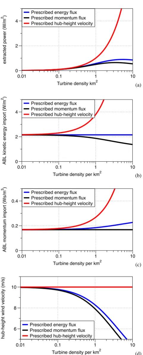
The fluxes of momentum and kinetic energy and the veloc-ities at the model heights were calculated for different wind turbine densities under the three assumptions. Figure 3 shows the response of the energy and momentum fluxes to changes in wind turbine density. Under assumption (1) the extracted power is a linear function of the number of wind turbines and increases accordingly. The import of kinetic energy and momentum also increase with increasing turbine density so as to offset extraction by the wind turbines, while hub-height velocities outside the wake volume remain constant.

The results of assumptions (2) and (3) resemble each other, both showing a saturating maximum in extracted wind power once a certain density of turbines is reached. Wind veloci-ties decrease with increasing turbine numbers, while kinetic energy and momentum input remain in the same order of magnitude.

(5)

F

tr ansf

er

F

acc

80 m 2000 m

d

Vtop

Vhub

F

turbine

F

sur face

Fig. 1. Schematic illustration of the vertical fluxes of horizontal

mo-mentum in the atmospheric boundary layer. Momo-mentum is imported from the upper atmosphere at the rateFaccand diffuses to lower

layers at the rateFtransfer, which is driven by the velocity gradient.

Wind turbines extract some of this momentum atvhubto generate

electrical energy (Fturbine).

We then compared these estimates for the case of a turbine-specific land areaAturbine= 10D·3D, where D is the diameter of the wind turbine, as suggested by Sta. Maria and Jacobson (2009). According to assumption (1), the downward momentum flux would need to increase 10-fold to 0.92 Ws m−3and the power input into the ABL would be 17.8 W m−2, which is also an increase by roughly an order of magnitude. Using assumptions (2) and (3) leads to rela-tively low changes in energy and momentum import at the top of the ABL. A comparison of the energy fluxes implied by the different assumptions at this specified turbine density is shown in Fig. 2

The results of assumption (1) pose the question of how the atmospheric circulation would be able to increase power generation by an order of magnitude. Because an explanation of the processes that would lead to such an increase has not been given yet, it seems unlikely that this drastic change is actually possible.

3 Comparison to climate model simulations

3.1 Climate model description

In order to evaluate which assumption is most reasonable and whether the atmosphere can generate much more power, we need to resort to a GCM that explicitly represents momen-tum balance constraints by being based on the Navier-Stokes equations of fluid dynamics. We use the climate model simu-lations of Miller et al. (2011) and compare their results with the ones derived by the 3 different scenarios. We are partic-ularly interested in how the boundary layer kinetic energy import responds to increased momentum extraction at the

Prescribed energy flux Prescribed momentum flux Prescribed hub-height velocity

extracted power (W/m

2 )

0 2 4

Turbine density km2

0.01 0.1 1 10

(a)

ABL

kinetic energy import (W/m

2 )

0 2 4

Turbine density per km2

0.01 0.1 1 10

(b)

ABL

momentum import (Ws/m

3 )

0 0.2 0.4

0.01 0.1 1 10

(c)

hub-height wind velocity (m/s)

6 8 10

0.01 0.1 1 10

(d)

Fig. 2. Comparison of the simple atmospheric boundary layer model

(6)

2000 m

d Pex=

23.2 _21.1

m/s

10

m/s

12.2

11.0

1.7

Jsurf ace

Jtransf er Jdiss

Jin

9.3

Vtop

Vhub

80 m

Prescribed hub-height velocity

2000 m

d Pex=

1.4

8.3

m/s

0.7

0.1

Jsurf ace

Jtransf er Jdiss

Jin

0.6

Vtop

Vhub

80 m

3.9

m/s

Prescribed momentum import

2000 m

d Pex=

2.2

9.6 m/s

1.1

0.2

Jsurf ace

Jtransf er Jdiss

Jin

0.9

Vtop

Vhub

80 m

4.5 m/s

Prescribed kinetic energy import

Fig. 3. Comparison of the kinetic energy fluxes for the 3 different

assumptions using a turbine spacing ofAturbine= 10D·3D, where

D= 61 m is the rotor diameter. Unless otherwise noted, all quanti-ties have the units W m−2.

surface. We can therefore determine if the increase in power generation predicted by the common method is supported by GCM results.

In these simulations, wind turbines are represented as an additional frictional force in the atmospheric boundary layer. Details of the study are described in Miller et al. (2011). The wind turbines, represented by the additional frictional param-eterCex, cause a frictional force on the atmospheric boundary layer,Ffric=ρ Cexv2. The conversion efficiency from wind

power extracted from the atmosphere to mechanical power of the turbine is estimated to be≈0.6 using the Betz limit. Extracted wind power per unit area is then

Pex =0.6·F ·v =0.6ρ Cexv3. (14) To represent the common method, wind velocities were taken from a control simulation without any additional fric-tion. Based on these velocities, the power output of a single turbine at each time step was calculated using Eq. (9). The total power extraction per unit surface area is then

Ptot = 1

Aturbine

Pex= 1

2ρ N ALand

CfArotorv3 (15) where _A 1

turbine is the turbine density on land. Comparing Eqs. (14) and (15) lets us derive the relationship between the friction parameterCexand the turbine density:

1 Aturbine

= 1.2Cex

CfArotor

. (16)

For example, a turbine density of 1 turbine per km2would correspond to a friction parameterCex= 0.0013. The kinetic energy import into the boundary layer of the GCM is diag-nosed using the energy balance Eq. (8), resulting in

Jin=DBL+Pex (17)

whereDBL is the rate of kinetic energy dissipation within the boundary layer andPexis the turbine associated power extraction.

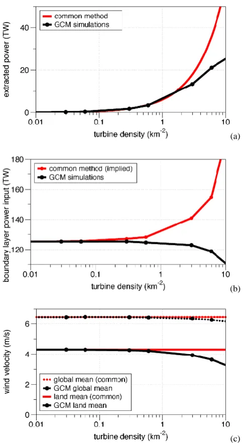
3.2 Results

The calculated power extraction as well as the influence of wind turbine density on boundary layer wind velocities and boundary layer power input is shown in Fig. 4. For low tur-bine densities, the common method and the GCM results lead to very similar results. As the turbine density increases, the estimates begin to diverge. During the process of kinetic en-ergy extraction, wind velocities decrease and therefore ki-netic energy extractability is reduced. The onset of the di-vergence takes place when≈10 % of the kinetic energy dis-sipated in the boundary layer is extracted by the turbines, consistent with the results of the simple model.

(7)

(a)

(b)

(c)

Fig. 4. Sensitivity of wind power extraction and consequences for

boundary layer flow from a set of climate model simulations in which all land regions are populated by wind turbines of differ-ent density. Shown are (a) mean power extraction by wind turbines,

(b) mean boundary layer kinetic energy import, and (c) mean global

wind velocities, and mean land wind velocities. The estimates of the common method are depicted by red lines and as modeled by the GCM are shown as black lines. Note the divergence of the two lines starting at≈2 turbines per km2, or a power extraction of 10 % of the total kinetic energy import into the boundary layer.

4 Discussion

This simple illustration as well as more complex GCM simulations show that accounting for the balance of mo-mentum and kinetic energy is critical to the quantification of large-scale extractability of wind power. Here, we will

discuss thermodynamic limits on wind energy generation rates within the atmosphere and link them with predictions made by GCM simulations. We then discuss how these pre-dictions meet the currently observed state of the atmosphere. Theory: Using well-established energetics of the atmo-sphere, the global generation rate of kinetic energy is esti-mated to be approximately 900 TW (Lorenz, 1955; Peixoto and Oort, 1992), about half of which is imported into the boundary layer. Less known thermodynamic derivations show that this rate of kinetic energy generation is at a max-imum value given the present-day radiative forcing gradi-ents, as demonstrated by simple theoretical considerations (Lorenz, 1960), box models (Paltridge, 1978; Lorenz et al., 2001) and general circulation model simulations (Kleidon et al., 2003, 2006). This therefore means that an increase in total atmospheric power generation due to wind turbine in-stallations as formulated in assumption (1) should not be ex-pected. Thermodynamic considerations therefore support the use of prescribed kinetic energy import or prescribed mo-mentum import, but rule out the assumption of a prescribed hub-height velocity, because it implies a significant increase in kinetic energy generation.

GCM results: This rather theoretical view is supported by the results of our GCM. In this more complex model, ki-netic energy generation does not increase due to additional wind turbine installations. Instead, the kinetic energy flux to the boundary layer decreases in response to very high wind turbine densities (see Fig. 4) and therefore contradicts the assumption of unaffected hub-height wind velocities. Every GCM is based on equations ensuring the conservation of mo-mentum, which is the main reason for the noted divergence in large-scale wind power estimates. So although the specific quantities of extractable wind power and related wind turbine density will certainly depend on specifications of the chosen GCM and its parameterization of wind turbines, the qualita-tive behavior should be reproducible with different models.

(8)

5 Conclusions

The ability of wind turbines of any size, quantity, or spa-tial arrangement to appropriate atmospheric kinetic energy is limited, first by the generation rate of kinetic energy in the atmosphere, and secondly, by the ability of these turbines to appropriate wind power from the atmospheric flow. The com-mon method assumes that the bulk velocity is not affected by the wind power extraction, thereby overestimating available wind power. Taken further, applying this “common method” for large-scale wind power estimates makes the resulting es-timate dependent on the turbine characteristics (swept-area, hub height, torque-to-electricity conversion efficiency, spa-tial arrangement), rather than the generation rate of motion within the atmosphere. While initially counter-intuitive, here we have illustrated why it is the generation rate of kinetic en-ergy in the atmosphere and the associated momentum fluxes, and not a more detailed understanding of wind velocities globally, that ultimately constrains wind power estimates to realizable limits.

It should also be clear that we are presently well below these limits to extraction. In 2008, the wind power produc-tion was 0.034 TW, or 0.2 % of the 2008 global energy de-mand of 16.5 TW (Arvizu et al., 2011). If wind farms con-tinue to increase in scale, our results suggest that physical limitations imposed by the atmosphere, estimated here using basic physical principles, will decrease and ultimately limit the power production of successive wind turbines. While it remains unclear how much energy the human population will demand in the future, studying these fundamental limits of renewable energy will ultimately present possible pathways to a renewable future. At a bare minimum though, to ensure that these estimates are relevant and scientifically defensible, careful attention must be paid to ensure that basic physical principles are being obeyed.

Acknowledgement. The authors thank Ryan Pavlick and Nathaniel Virgo for their comments which improved this manuscript.

The reviewers (Valerio Lucarini, Klaus Hasselmann, Daniel Kirk-Davidoff and two anonymous referees) also aided in clarifying several concepts and conclusions that appear in the final version of this manuscript. This work has been partially supported by the Helmholtz research alliance “Planetary Evolution and Life”.

Edited by: H. Held

References

Arvizu, D., Bruckner, T., Edenhofer, O., Estefen, S., Faaij, A., Fischedick, M., Hiriart, G., Hohmeyer, O., Hollands, K. G. T., Huckerby, J., Kadner, S., Killingtveit, A., Kumar, A., Lewis, A., Lucon, O., Matschoss, P., Maurice, L., Mirza, M., Mitchell, C., Moomaw, W., Moreira, J., Nilsson, L. J., Nyboer, J., Pichs-Madruga, R., Sathaye, J., Sawin, J., Schaeffer, R., Schei, T.,

Schl¨omer, S., Seyboth, K., Sims, R., Sinden, G., Sokona, Y., von Stechow, C., Steckel, J., Verbruggen, A., Wiser, R., Yamba, F., and Zwickel, T.: Technical Summary, in: IPCC Special Report on Renewable Energy Sources and Climate Change Mitigation, edited by: Edenhofer, O., Pich-Madruga, R., Sokona, Y., Sey-both, K., Matschoss, P., Kadner, S., Zwickel, T., Eickemeier, P., Hansen, G., Schl¨omer, S., and von Stechow, C., Cambridge Uni-versity Press, Cambridge, UK and New York, NY, USA, 2011. Archer, C. L. and Jacobson, M. Z.: Evaluation of global wind power,

J. Geophys. Res., 110, D12110, doi:10.1029/2004JD005462, 2005.

Keith, D., DeCarolis, J., Denkenberger, D., Lenschow, D., Maly-shev, S. L., Pacala, S., and Rasch, P.: The influence of large-scale wind power on global climate, P. Natl. Acad. Sci., 101, 16115– 16120, 2004.

Kleidon, A., Fraedrich, K., Kunz, T., and Lunkeit, F.: The atmo-spheric circulation and states of maximum entropy production, Geophys. Res. Lett., 30, 2223, doi:10.1029/2003GL018363, 2003.

Kleidon, A., Fraedrich, K., Kirk, E., and Lunkeit, F.: Maximum en-tropy production and the strength of the boundary layer exchange in an atmospheric general circulation model, Geophys. Res. Lett., 33, L06706, doi:10.1029/2005GL025373, 2006.

Leithead, W.: Wind energy, Philos. T. Roy. Soc. A, 365, 957–970, 2007.

Liu, W. T., Tang, W., and Xie, X.: Wind power distri-bution over the ocean, Geophys. Res. Lett., 35, L13808, doi:10.1029/2008GL034172, 2008.

Lorenz, E.: Available potential energy and the maintenance of the general circulation, Tellus, 7, 271–281, 1955.

Lorenz, E.: Generation of available potential energy and the inten-sity of the global circulation, Dynam. Climate, Pergamon Press, Oxford, UK, 86–92, 1960.

Lorenz, R., Lunine, J., Withers, P., and McKay, C.: Titan, Mars, and Earth: entropy production by latitudinal heat transport, Geophys. Res. Lett., 28, 415–418, 2001.

Lu, X., McElroy, M. B., and Kiviluoma, J.: Global potential for wind-generated electricity, P. Natl. Acad. Sci., 106, 10933, doi:10.1073/pnas.0904101106, 2009.

Miller, L. M., Gans, F., and Kleidon, A.: Estimating maxi-mum global land surface wind power extractability and as-sociated climatic consequences, Earth Syst. Dynam., 2, 1–12, doi:10.5194/esd-2-1-2011, 2011.

Paltridge, G. W.: The steady-state format of global climate, Q. J. Roy. Meteorol. Soc., 104, 927–945, 1978.

Peixoto, J. P. and Oort, A. H.: Physics of climate, American Institute of Physics, Springer-Verlag, New York, USA, 1992.

Sta. Maria, M. R. V. and Jacobson, M.: Investigating the effect of large wind farms on energy in the atmosphere, Energies, 2, 816– 838, 2009.

Stull, R. B.: An introduction to boundary layer meteorology, Kluwer Academic Publishers, Dordrecht, The Netherlands, 1988. Wang, C. and Prinn, R. G.: Potential climatic impacts and reliability