www.nonlin-processes-geophys.net/20/793/2013/ doi:10.5194/npg-20-793-2013
© Author(s) 2013. CC Attribution 3.0 License.
Nonlinear Processes
in Geophysics
A variational formulation for translation and assimilation of
coherent structures
M. Plu
Laboratoire de l’Atmosphère et des Cyclones, UMR8105, Unité mixte CNRS/Météo-France/Université de La Réunion, and CNRM-GAME, Météo-France/CNRS, Toulouse, France
Correspondence to: M. Plu ([email protected])
Received: 26 November 2012 – Revised: 6 September 2013 – Accepted: 6 September 2013 – Published: 17 October 2013
Abstract. The assimilation of observations from teledetected images in geophysical models requires one to develop al-gorithms that would account for the existence of coherent structures. In the context of variational data assimilation, a method is proposed to allow the background to be translated so as to fit structure positions deduced from images. Trans-lation occurs as a first step before assimilating all the obser-vations using a classical assimilation procedure with specific covariances for the translated background. A simple valida-tion is proposed using a dynamical system based on the one-dimensional complex Ginzburg–Landau equation in a regime prone to phase and amplitude errors. Assimilation of obser-vations after background translation leads to better scores and a better representation of extremas than the method with-out translation.
1 Introduction
Numerical prediction of geophysical flows (meteorology, oceanography, hydrology, etc.) requires an analysis proce-dure. Its purpose is to obtain an optimal initial state at a given instant from which the forecast is computed. Such an analysis is generally provided by correcting a previous fore-cast (the background) by observations: this is the assimila-tion step of observaassimila-tions. Most data assimilaassimila-tion algorithms rely on the best linear unbiased estimation (BLUE, Tala-grand, 1997), which is a statistical estimator that requires the prior knowledge of the bias and variance of the errors affecting the input data. The BLUE achieves Bayesian esti-mation if the distribution of errors, taken as a whole, is Gaus-sian. The BLUE is the background for powerful algorithms, such as sequential Kalman (1960) filtering and variational
assimilation (Le Dimet and Talagrand, 1986; Talagrand and Courtier, 1987).
Conventional observations and satellite radiances defined as punctual values are the essential input data for such anal-ysis. Observation errors are usually presumed to be uncorre-lated. As a consequence, the assimilated pixels from a satel-lite image are undersampled so that to guarantee that their errors are enough uncorrelated. Still, geophysical flows often contain coherent structures that teledetected images may ex-hibit, as for example in the atmosphere for tropical cyclones or midlatitude storms (Plu et al., 2008). Consistent with this statement, Hoffman et al. (1995) proposed to separate mete-orological forecast errors into displacement error, amplitude error and residual error. However, the position, size and shape of structures cannot be assimilated correctly by algorithms derived from the BLUE (Titaud et al., 2010; Michel, 2011). A reason, among others, for this deficiency is that error dis-tributions in flows with finite-amplitude coherent structures diverge from Gaussianity (Beezley and Mandel, 2008).
Some studies have investigated possible means of assim-ilating features from satellite images. Bogussing is such a technique: pseudo-observations deduced from an observed coherent structure are assimilated as conventional observa-tions (wind, humidity, etc.). The assumpobserva-tions that link the image to the pseudo-observation are often simplified (Hem-ing et al., 1995; Michel, 2011; Montroty et al., 2008), and such methods are not fully objective. Michel (2011) con-cluded about the severe limitations of bogussing.
background remains small. Ravela et al. (2007) developed a two-step method in which the background is first aligned to an observed image, before treating amplitude errors using a conventional ensemble Kalman filter. Beezley and Mandel (2008) inserted a morphing analysis step between sequential Kalman filter steps, in order to fit a model state to observed images.
These promising studies emphasize the need to develop as-similation methods that would treat properly the errors asso-ciated with coherent structures. In theory, the most satisfac-tory approach would be to relax the Gaussian assumption and to develop fully Bayesian estimators. But, assimilation tech-niques must remain simple in order to deal effectively with numerical models that have very high degrees of freedom. A reasonable approach is to try to adapt the existing assimila-tion procedures (Kalman filter and variaassimila-tional) to take dis-placement errors into account. The present article proposes and tests a method to translate the background in the context of variational assimilation.
In the first section, the concept of background transla-tion is formulated and a method of resolutransla-tion is proposed. In the second section, a validation is provided for a one-dimensional numerical system prone to phase errors. Possi-ble extension to a realistic context is then discussed before the conclusion.
2 Method for background translation 2.1 Notations and general formulas for data
assimilation
The model state vector is notedx=(xi)i=1...N. At a given instant, a backgroundxb=(xb
i)i=1...N and a set ofp obser-vationsyo=(yo
j)j=1...pare known. If background errors and observation errors are supposed to be uncorrelated, and if they are known up to second-order statistical moments, the optimal analysisxamay be obtained as:
xa=xb+BHT(HBHT +R)−1[yo−Hxb], (1) where H is the observation operator and B and R are, re-spectively, the background covariance error and observation covariance error matrices. BHT(HBHT+R)−1=K=(ki,j) is the gain matrix. This is the equation used in the analy-sis step of sequential Kalman filtering. The variational form of Eq. (1) consists in minimizing the quadratic cost function J =Jo+Jb:
J(x)=
(Hx−yo)TR−1(Hx−yo)+(x−xb)TB−1(x−xb). (2) 2.2 A variational approach for translating structures in
the background
The preceding equations will be adapted here to allow coher-ent structures in the background field to be translated onto
the corresponding observed structures. Let us define a local translation as the translation of a finite-length segment. What is sought is the sum of local translations that would make coherent structures in the background fit the observed struc-tures. A first hypothesis is to build a transformed background by applying a surjective function to indices:
xbt=(xib+t (i)), (3) wheret is an integer function[1, N] 7→] −N/2, N/2]such as 1≤i+t (i)≤N ∀i∈ [1, N]. The functiont is not given a priori. It is a supplementary degree of freedom that must be estimated by the method. A local translation corresponds to a constant value fort over a segment and 0 elsewhere. In the general context of geophysical background fields, such a translation is not satisfactory since it may generate a dis-continuous transformed background field xbt. The function
t should therefore be a compromise between the following constraints:
– the position of every coherent structure in the trans-formed backgroundxbtshould match the position of a
coherent structure in the observed image, – t should be the sum of local translations,
– the transformed backgroundxbtshould be smooth. It is assumed that these constraints may be accounted for by minimizing a cost function Jt. The extension of vari-ational assimilation (Eq. 2) to allow background transla-tion may thus be resolved by minimizing the cost functransla-tion J =Jo+Jb+Jt:
J(x, t )=(Hx−yo)TR−1(Hx−yo)+
(x−xbt)TB−t 1(x−xbt)+Jt(t ), (4) where Bt would depend on the translation (Ravela et al., 2007). The background is allowed to be translated in theJb
term, which is expected to make sense wherever there is in-consistency between a structure position in the observations and in the background. Although several definitions could be possible, theJt(t )term is proposed as:
Jt(t )=w1
N−1
X
i=2
(t (i)−t (i−1))2t (i)2+
w2
N−1
X
i=2
(t (i)−t (i−1))2 , (5)
wherew1 andw2are positive parameters. Thew1 term of
Eq. (5) has three desirable properties:
– translating a large zone has a similar cost as translating a small zone,
– it is differentiable.
Thew2term reaches low values for local translations.
More-over, it gives a high cost to the irregular t function, thus smoothing the transformed background xbt. As a conse-quence, Eq. (5) provides a cost function to account for the desirable constraints of functiont.
Although Eq. (4) seems to be a reasonable formula to account for structure position errors in the background, its numerical resolution is far from being obvious.J is not a quadratic function of(x, t ): the existence of a unique mini-mum is not sure. However, if the transformationtis fixed,J is a quadratic function ofx. A two-step method is thus pro-posed to get an optimal(xa, ta):J is minimized first along
tso as to get a transformationta, and thenxais obtained by minimizingJ for this given fieldta.
Step 1. An optimaltais searched, such as minimizing F(t )=J(xbt, t )=(Hxbt−yo)TR−1(Hxbt−yo)+
N−1
X
i=2
(t (i)−t (i−1))2w1t (i)2+w2
. (6)
The purpose of this step is to obtain a satisfactoryt func-tion as a compromise between fitting the transformed back-groundxbtto the observed imageyo, limiting the amplitude
of translations and leading to a smooth transformed back-ground xbt. The observations taken into account in step 1 may be restricted to the images according to which the back-ground coherent structures are wished to be corrected.
SinceF is a discrete function with positive values, it ad-mits a global minimum value for one or several transforma-tion vectors t. Minimization could simply be achieved by spanning all the possiblet values, which would be a perfect but inefficient method. Another approach is to find a local minimum using a solver for minimization, like the one from Gilbert and Lemaréchal (1989). For this purpose,tis allowed to have real values. It is also necessary thatF(Eq. 6) is con-tinuous and differentiable, which is guaranteed if the term Jo(xbt)is computed using cubic interpolations. IfFadmits
several local minimas, the minimization solver may find dif-ferent solutions, depending on the first guess vectort that initiates the solver. To reach a reasonable solution, and in ac-cordance with the purpose of background translation, a first guesstused for minimization is automatically defined. It is a zero vector except for the points where Hxbreaches the po-sition of the centre of a coherent structure: at these points the transformation connects to the centre of the nearest coherent structure in the observation. After minimization, the values
t (i)are rounded to integer values. This method is general enough to be applied to many geophysical contexts, provided there is the possibility of identifying coherent structures in
Thew2-term reaches low values for local translations.
More-over it gives a high cost to irregulartfunction, thus smooth-ing the transformed background xbt. As a consequence, Eq. 5 provides a cost function to account for the desirable constrains of functiont.
155
Although Eq. 4 seems to be a reasonable formula to ac-count for structure position errors in the background, its nu-merical resolution is far from being obvious. J is not a quadratic function of(x,t): the existence of a unique mini-mum is not sure. However, if the transformationtis fixed,J
160
is a quadratic function ofx. A two-step method is thus pro-posed to get an optimal(xa,ta): J is minimized first along tso as to get a transformationta, and thenxais obtained by
minimizingJ for this given fieldta.
Step 1. An optimaltais searched such as minimizing
165
F(t) =J(xbt,t) = (Hxbt−yo)TR−1(Hxbt−yo)+
N−1
X
i=2
(t(i)−t(i−1))2 w1t(i)2+w2, (6)
The purpose of this step is to obtain a satisfactoryt func-tion as a compromise between fitting the transformed back-groundxbtto the observed imageyo, limiting the amplitude of translations, and leading to a smooth transformed
back-170
groundxbt. The observations taken into account in step 1
may be restricted to the images according to which the back-ground coherent structures are wished to be corrected.
SinceF is a discrete function with positive values, it ad-mits a global minimum value for one or several
transforma-175
tion vectorst. Minimization could be simply be achieved by spanning all the possibletvalues, which would be a perfect but inefficient method. Another approach is to find a local minimum using a solver for minimization, like the one from Gilbert and Lemarchal (1989). For this purpose,tis allowed
180
to have real values. It is also necessary thatF(Eq. 6) is con-tinuous and differentiable, which is guaranteed if the term
Jo(xbt) is computed using cubic interpolations. If F
ad-mits several local minimas, the minimization solver may find different solutions depending on the first guess vectortthat
185
initiates the solver. To reach a reasonable solution and in ac-cordance with the purpose of background translation, a first guesstused for minimization is automatically defined. It is a zero-vector except for the points whereHxbreaches the po-sition of the centre of a coherent structure: in these points the
190
transformation connects to the centre of the nearest coherent structure in the observation. After minimization, the values
t(i) are rounded to integer values. This method is general enough to be applied to many geophysical contexts, provided there is the possibility to identify coherent structures in
mod-195
eled and observed fields. Fig. 1 shows an idealized result of step 1, defining the centre of the coherent structure as a local maximum. Translation applies so that the tranformed
back-100 110 120 130 140 150 160 170
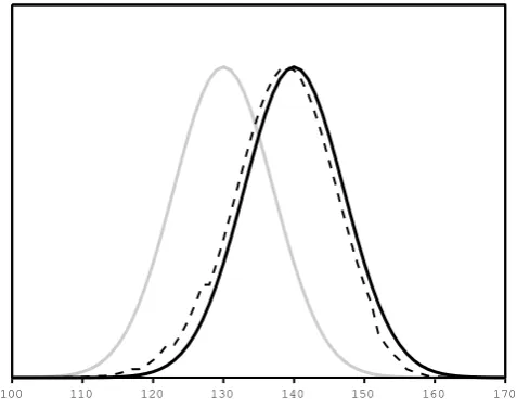
Fig. 1. Illustration of the translation method applied to an
ideal-ized function. The observed vectoryo(solid black curve) and the backgroundxb (solid light-grey curve) are bell-shaped functions, centered at different positions. The translated background resulting from the step-1 method is in dash. The algorithm uses the follow-ing parameters:w1= 1.5 10−3,w2= 4, corresponding to a typical position error of10grid points, like in the following parts of the article.His the identity matrix.
satisfactory and in particular, the transformed background is
200
reasonably smooth. In such an idealized context, the solution should be a uniform translation, for which the cost function given in Eq. 6 is null. The non-perfect result in Fig. 1 re-veals some minor defects of the method of resolution, due to non-convexity of Eq. 6 and to the fact that the result of
205
minimization depends on the input vector.
The results should depend on the parametersw1 andw2
and it is important to define and calibrate them properly. The parameterσtis introduced, which is a typical value for
ac-ceptable translation of the background. This value may be
210
defined by the user or derived from background statistics (see implementation further). Since the first term of Eq. 5 should constrain the amplitude of local translations, the parameter
w1 should be linked toσt. Consider a single local
transla-tion whose value isσtover a segment of a given size, and
215
that, at the boundaries of this segment,t decreases one by one towards 0. The cost function of such a local transla-tion is twice the sum of integers from0toσt, which equals w1σt(σt+ 1)(2σt+ 1)/3. For practical purpose, this
expres-sion is approximated as2w1σt3/3. To calibrate properly the
220
different terms of F (Eq. 6), the expression w1= 3/2σ−t3
is obtained. Thenw2 is adjusted so as to obtain reasonably
smooth solutions.
Step 2. Given the vectorta from step 1, the analysisxa
is then obtained by minimizingJ(x,ta)alongx.
Accord-225
ing to Eq. (4), Bt is the error covariance matrix between
Fig. 1. Illustration of the translation method applied to an
ideal-ized function. The observed vectoryo(solid black curve) and the backgroundxb (solid light-grey curve) are bell-shaped functions, centered at different positions. The translated background resulting from the step-1 method is in dash. The algorithm uses the following parameters:w1=1.5×10⁻³,w2=4, corresponding to a typical
position error of 10 grid points, as in the following parts of the arti-cle. H is the identity matrix.
modelled and observed fields. Figure 1 shows an idealized result of step 1, defining the centre of the coherent structure as a local maximum. Translation applies, so that the tran-formed background fits well to the observation. The method seems to be satisfactory and, in particular, the transformed background is reasonably smooth. In such an idealized con-text, the solution should be a uniform translation for which the cost function given in Eq. (6) is null. The non-perfect re-sult in Fig. 1 reveals some minor defects in the method of resolution, due to the non-convexity of Eq. (6) and the fact that the result of minimization depends on the input vector.
The results should depend on the parametersw1andw2,
and it is important to define and calibrate them properly. The parameterσt is introduced, which is a typical value for
ac-ceptable translation of the background. This value may be defined by the user or derived from background statistics (see implementation further). Since the first term of Eq. (5) should constrain the amplitude of local translations, the pa-rameterw1 should be linked to σt. Consider a single local
translation whose value isσtover a segment of a given size,
and that, at the boundaries of this segment,t decreases one by one towards 0. The cost function of such a local transla-tion is twice the sum of integers from 0 toσt, which equals
w1σt(σt+1)(2σt+1)/3. For practical purposes this
expres-sion is approximated as 2w1σt3/3. To calibrate properly the
different terms of F (Eq. 6), the expressionw1=3/2σt−3
is obtained. Thenw2 is adjusted so as to obtain reasonably
Step 2. Given the vectorta from step 1, the analysisxa is then obtained by minimizingJ(x, ta)alongx. According to Eq. (4), Bt is the error covariance matrix between trans-formed background. Bt may be static or it may depend on the transformation computed in step 1. How to compute at -dependent Bt is not obvious (Ravela et al., 2007) and poses numerical issues. It is thus assumed that Bt=B0, like B, is static. If the error is supposed to be the sum of displacement and amplitude errors (Hoffman et al., 1995), B0 should rep-resent the covariance of amplitude errors. In other words, B0 may be obtained after eliminating the part of error due to dis-placement errors of coherent structures. A possible method to compute the B0matrix would be similar to the one for B. The most common method uses an ensemble of coupled forecasts valid at the same time (Parrish and Derber, 1992; Pereira and Berre, 2006), starting from different initial conditions. B is built from the covariance of the differences between the cou-pled forecasts. To compute B0, one of the coupled forecasts is
translated towards the other one using the algorithm of step 1, thus attempting to remove displacement errors of coherent structures. The same algorithm as in step 1 should be used to identify the position of coherent structures in forecasts. B is built from the covariance of the differences between the translated forecast and the other one.
Assuming Bt=B0as static and K0the associated gain ma-trix, step 2 is also equivalent to the direct formula:
xa=xbt+K0[yo−Hxbt],
or
xia=
xib+t (i)+ p X
j=1
k0i,j "
yjo− N X
l=1
hl,jxlb+t (l) #
∀i∈ [1, N]. (7)
Like the one proposed by Ravela et al. (2007), this two-step method attempts to first fit the background to observa-tions and then to apply a classical assimilation procedure. The equations here apply to a variational context and the method of resolution seems to be simpler than the one of Ravela et al. (2007). The cost functionJ does not necessar-ily admit a unique minimum and the two-step procedure is not proven to lead to a local minimum ofJ. However, this two-step procedure leads to a unique solution, and arguments have been provided that it should not be far from an optimal one. In order to be more confident about the method, a vali-dation is now proposed.
3 Validation on a one-dimensional system
The method will be applied to a one-dimensional dynamical system, in order to prove the concept of background trans-lation and to reveal some possible limitations. Such a one-dimensional system does not provide images, which are two-dimensional by definition. However, the extreme values of
the wave packets that evolve in the one-dimensional system may play a similar role as the coherent structures seen in satellite images. The main reason for restricting to one di-mension is that the assimilation procedure (spatial correla-tions) is highly simplified and cost-effective.
3.1 Dynamical system
The one-dimensional system is the complex Ginzburg– Landau equation. For some relevant parameters, this weakly nonlinear system simulates coherent structures and is sensi-tive to initial conditions. The evolution of the complex func-tionu(z, t )on a periodic segment is given by:
∂u
∂t =u+(1+iα) ∂2u
∂z2 −(1+iβ)|u|
2u. (8)
The horizontal dimensionz and timet are, respectively, expressed in m and s. The stability and the chaotic proper-ties of the system depend on the parametersαandβ, which are chosen asα=2 andβ= −1.5 in all the following exper-iments. Such a regime is absolutely unstable (Weber et al., 1992), with a Lyapunov exponent 1.6×10⁻²s−1equivalent to a doubling time of small perturbations around 45 s. Nu-merical integrations confirm the sensitivity to initial condi-tions of phase and amplitude of the traveling wave packets. Such a model provides errors of position and amplitude of coherent structures that will be suitable for testing various assimilation algorithms. In such model fields, the centres of coherent structures are simply identified as the local maxi-mas and the local minimaxi-mas.
The equation is integrated over an N=512-point peri-odic segment of L=100 m length. Numerical integration relies on exponentional time differencing of second order applied to the Fourier coefficients of u. Let us define the nonlinear term of Eq. (8) as the function G(z, t )=(1+
iβ)|u(z, t )|2u(z, t ), andu˜k(t )(respG˜k(t )) the Fourier coef-ficients ofu(z, t )(resp (G(z, t )) at instantt. The method for time integration for each indexkis:
˜
uk(t+1t )= ˜
uk(t )eqk1t+ [ ˜Gk(t )(1+qk1t )eqk1t−1−2qk1t+ ˜
Gk(t−1t )(−eqk1t+1+qk1t )]/(qk21t ), (9) whereqk=1−(1+iα)(2π k/L)2, and the time step is1t= 0.05 s.
3.2 Error statistics
0
-10 10 20 30
-20 -30
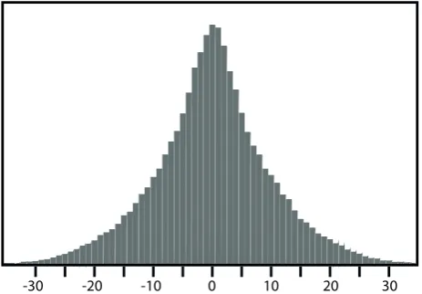
Fig. 2. Distribution of difference of positions between the closest
maximas and between the closest minimas (ie coherent structures) in the10000coupled forecasts.
translation approach described in step 1. The background er-ror covariances are supposed to be homogeneous over the do-main. TheBmatrix is computed from covariance of the dif-ference between the10000coupled forecasts. TheB′matrix
is computed from covariance of the difference between the
315
10000translated coupled forecasts and the original ones. The local variance changes significantly after translation: while it is0.070forB, it gets down to0.043forB′. The variance of
the translated background error is much lower than the orig-inal variance of background error, reflecting the reduction, if
320
not removal, of displacement error.
Depending on the assimilation experiments, background error covariance matrices are supposed to be diagonal or not. It has been verified that statistics do not depend much on the amplitude of the initial white-noise. In addition, the typical
325
value for translation σt is deduced from the distribution of difference of positions between the closest local maxima in the coupled forecasts (Fig. 2). Its standard deviation yields the uniform parameter σt= 10 (gridpoint unit) used in the following assimilation experiments.
330
The observation error covariance matrixRis supposed to be diagonal (no spatial correlation) and uniform.
3.3 Validation
A nature run is computed using the model configuration de-scribed previously. 1001 nature state vectors are thus
ob-335
tained, one every100s. At each instant,
– an observation state vector is computed as the nature perturbed by some random small-amplitude noise, this observation is assumed to be both the image towards which background may be translated (step 1) and the
340
observation vector (with or without undersampling) that will be assimilated (step 2),
– a model background is obtained as the100s model in-tegration from the previous instant, starting from the nature state vector perturbed by some random
small-345
amplitude noise.
The nature run serves as a reference from which error values are computed. It follows from this very simple system that the observation operatorHis a unity matrix. Assimilation of observations in the background for the1000instants is done
350
using different methods. The experiments with background translation use the step-1 algorithm described in section 2.2, withw1= 1.5 10−3(corresponding to σt= 10) and w= 4 (for sufficient smoothness deduced from tests like in Fig. 1). Eight experiments (Tab. 1) are compared by measuring a
355
score, as the r.m.s of analysis error (difference between the assimilated and the nature state vectors over the1000cases). Since translations do not apply at the boundaries (Eq. 3), only the points at32gridpoints inside the segment are used for score computation. The ability of the experiments to
re-360
produce the coherent structures (extrema) of the nature run (Fig. 4) is also compared. The B matrix may be diago-nal, or spatial correlations may be taken into account (non-diagonal). Another option is whether the whole observation state vector is assimilated or whether it is undersampled (1
365
point over 5) in step 2, in order to mimic the classical under-sampling of satellite images.
Fig. 3 shows the distribution of background error before and after translation, deduced from the 1000-instants sam-ple. The translation step reduces significantly the standard
370
deviation (0.17instead of 0.26), which is consistent with the reduction of displacement error discussed in section 3.2. The distribution error is not initially Gaussian, with skewness
−0.045and kurtosis4.21(a Gaussian distribution has skew-ness0and kurtosis3). After translation, skewness is−0.16
375
and kurtosis is6.3, which means that the Gaussianity of the background error distribution after translation is slightly de-graded. Although it has been wished that translation would improve Gaussianity of background error in order to better apply the BLUE, this result does not prevent from testing
as-380
similation.
An attempt has also been done to iterate several times the two-step method, using the ouput(xa,ta)as input of a sec-ond processing of steps 1 and 2. The results over the1000 test cases was that translation was rarely modified after
an-385
other step 1 and, if it changed, it was only a few grid points. No significant improvement may thus be expected from fur-ther iterations of the two-step method.
Tab. 1 and Fig. 4 illustrate the method and compare it to classical variational assimilation. For every experiments, the
390
scores (r.m.s of analysis error) remain between the r.m.s of observation error (0.034) and the r.m.s of background er-ror (0.26), which means that the assimilation procedure is suboptimal, probably due to non-linearities of the Ginzburg-Landau system. If two equivalent experiments are compared,
395
one with and one without translation, the one with
transla-Fig. 2. Distribution of difference of positions between the closest
maximas and between the closest minimas (i.e. coherent structures) in the 10 000 coupled forecasts.
The background error covariances are obtained from a sample of 10 000 independent forecasts at lead time 100 s. For each initial state, a coupled initial state is obtained after addition of small-amplitude white noise and a coupled fore-cast after simulation of this initial state. For each forefore-cast, a translated coupled forecast is obtained after translation of the coupled forecast towards the unperturbed forecast, us-ing the translation approach described in step 1. The back-ground error covariances are supposed to be homogeneous over the domain. The B matrix is computed from covariance of the difference between the 10 000 coupled forecasts. The B0matrix is computed from covariance of the difference be-tween the 10 000 translated coupled forecasts and the original ones. The local variance changes significantly after transla-tion: while it is 0.070 for B, it gets down to 0.043 for B0. The variance of the translated background error is much lower than the original variance of background error, reflecting the reduction, if not removal, of displacement error.
Depending on the assimilation experiments, background error covariance matrices are supposed to be diagonal or not. It has been verified that statistics do not depend much on the amplitude of the initial white noise. In addition, the typical value for translation σt is deduced from the distribution of
difference of positions between the closest local maxima in the coupled forecasts (Fig. 2). Its standard deviation yields the uniform parameter σt=10 (gridpoint unit) used in the
following assimilation experiments.
The observation error covariance matrix R is supposed to be diagonal (no spatial correlation) and uniform.
3.3 Validation
A nature run is computed using the model configuration de-scribed previously. 1001 nature state vectors are thus ob-tained, one every 100 s. At each instant,
– an observation state vector is computed as the na-ture perturbed by some random small-amplitude noise. This observation is assumed to be both the image to-wards which a background may be translated (step 1) and the observation vector (with or without undersam-pling) that will be assimilated (step 2),
– a model background is obtained as the 100 s model in-tegration from the previous instant, starting from the nature state vector perturbed by some random small-amplitude noise.
The nature run serves as a reference from which error values are computed. It follows from this very simple system that the observation operator H is a unity matrix. Assimilation of observations in the background for the 1000 instants is done using different methods. The experiments with background translation use the step-1 algorithm described in Sect. 2.2, withw1=1.5×10⁻³(corresponding toσt=10) andw=4
(for sufficient smoothness deduced from tests like in Fig. 1). Eight experiments (Table 1) are compared by measuring a score as the r.m.s. of analysis error (difference between the assimilated and the nature state vectors over the 1000 cases). Since translations do not apply at the boundaries (Eq. 3), only the points at 32 gridpoints inside the segment are used for score computation. The ability of the experi-ments to reproduce the coherent structures (extrema) of the nature run (Fig. 4) is also compared. The B matrix may be diagonal, or spatial correlations may be taken into account (non-diagonal). Another option is whether the whole obser-vation state vector is assimilated or whether it is undersam-pled (1 point over 5) in step 2, in order to mimic the classical undersampling of satellite images.
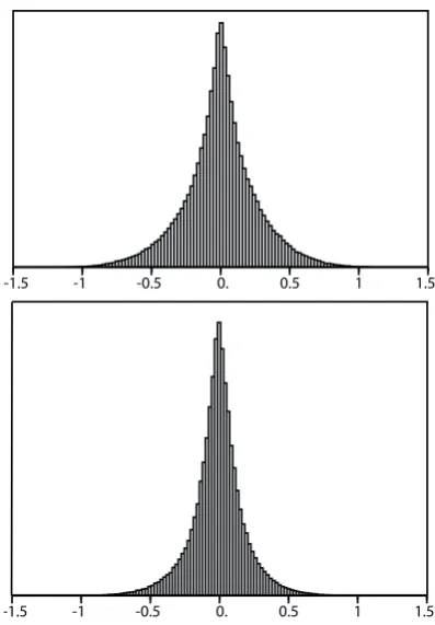
Figure 3 shows the distribution of background error before and after translation, deduced from the 1000-instants sam-ple. The translation step reduces significantly the standard deviation (0.17 instead of 0.26), which is consistent with the reduction in displacement error discussed in Sect. 3.2. The distribution error is not initially Gaussian, with skewness −0.045 and kurtosis 4.21 (a Gaussian distribution has skew-ness 0 and kurtosis 3). After translation, skewskew-ness is−0.16 and kurtosis is 6.3, which means that the Gaussianity of the background error distribution after translation is slightly de-graded. Although it has been wished that translation would improve the Gaussianity of background error in order to bet-ter apply the BLUE, this result does not prevent one from testing assimilation.
An attempt has also been made to iterate several times the two-step method, using the ouput(xa, ta)as the input of a second processing of steps 1 and 2. The results over the 1000 test cases was that translation was rarely modified after an-other step 1 and, if it changed, it was only by a few grid points. No significant improvement may thus be expected from further iterations of the two-step method.
-1.5 -1 -0.5 0. 0.5 1 1.5
-1.5 -1 -0.5 0. 0.5 1 1.5
Fig. 3. Distribution of background error before translation (top) and
after translation (bottom).
Table 1. Description of the eight assimilation experiments:
assump-tion for theBmatrix, translation approach (no, T1 or T2), distance (in gridpoints) between the observations that are assimilated, score (r.m.s of analysis error) of the experiment.
number B translation obs. distance score
exp1 non-diagonal no 1 0.042
exp2 non-diagonal no 5 0.213
exp3 non-diagonal yes 1 0.040
exp4 non-diagonal yes 5 0.135
exp5 diagonal no 1 0.091
exp6 diagonal no 5 0.238
exp7 diagonal yes 1 0.061
exp8 diagonal yes 5 0.151
tion has better scores than the one without translation, and it better represents the extremas. The example of translated
background (Fig. 4) confirms the results shown in Fig. 1: the extremas in the translated background fit well the ones from 400
the observation, while preserving smoothness. The analysis after background translation seems to be less smooth than without, but the amplitude of the irregularities remain small. The experiments with and without background translation will now be compared in detail. The experiments exp1 and 405
exp3 are designed with the most complete assumptions: hor-izontal correlations are full (BandB′are non-diagonal) and every observed points are assimilated. Still, the score (Tab. 1) is improved in exp3 (with background translation) compared to exp1 (without background translation) and most of the ex-410
tremas and slopes (upper panels of Fig. 4) are better repre-sented using background translation. The experiments exp2, exp4, exp5 and exp7 are closer to classical geophysical mod-els, either the observations are undersampled before assim-ilation or the background error covariance matrices are di-415
agonal. Tab. 1 shows that each experiment with background translation (exp4 and exp7 resp.) perform better than the cor-responding one without (exp2 and exp5 resp.). In particular, the extremas in exp7 (Fig. 4, bottom-right panel) are far bet-ter reproduced than in exp5 (Fig. 4, bottom-left panel), and 420
nearly as good as in exp3 (Fig. 4, upper-right panel). Back-ground translation without horizontal correlations performs nearly as well as a classical assimilation with background translation. To some extent, this result suggests that back-ground translation corrects position errors, and amplitude er-425
rors may be corrected without spatial correlations.
Fig. 5 shows another example, for which the local transla-tions to be sought are positive at some points (peak around abscissa160) and negative at some other points (peak around abscissa250). In such a case, the transformed background 430
(left panels of Fig. 5, dashed lines) correctly fits the peaks from the background to the observations. The resulting as-similation procedure leads to improved results compared to assimilation without background translation (Fig. 5).
4 Discussion on the possible implementation in a
mete-435
orological model
The method that has been described is sufficiently general to be applied on many geophysical models. The purpose of this section is to present and discuss how the method could be applied to a specific variational meteorological assimilation 440
scheme. It is assumed that an algorithm is available to detect coherent structures in images and in numerical model outputs (Plu et al., 2008; Michel, 2011).
Coherent structures in meteorology may be observed in two-dimensional fields, such as satellite or radar images. But 445
meteorological models are three-dimensional. It is thus suf-ficient to let translation to be two-dimensional: translated background points are not allowed to go through vertical lev-els. The translation fields are computed by minimizing Eq. 6.
Fig. 3. Distribution of background error before translation (top) and
after translation (bottom).
scores (r.m.s. of analysis error) remain between the r.m.s. of observation error (0.034) and the r.m.s. of background er-ror (0.26), which means that the assimilation procedure is suboptimal, probably due to nonlinearities of the Ginzburg– Landau system. If two equivalent experiments are compared, one with and one without translation, the one with transla-tion has better scores than the one without translatransla-tion, and it better represents the extremas. The example of translated background (Fig. 4) confirms the results shown in Fig. 1: the extremas in the translated background fit well with the ones from the observation, while preserving smoothness. The analysis after background translation seems to be less smooth than without, but the amplitude of the irregularities remains small.
The experiments with and without background translation will now be compared in detail. The experiments exp1 and exp3 are designed with the most complete assumptions: hor-izontal correlations are full (B and B0are non-diagonal) and
all observed points are assimilated. Still, the score (Table 1) is improved in exp3 (with background translation) com-pared to exp1 (without background translation), and most of the extremas and slopes (upper panels of Fig. 4) are better represented using background translation. The experiments exp2, exp4, exp5 and exp7 are closer to classical geophysical models: either the observations are undersampled before as-similation, or the background error covariance matrices are
Table 1. Description of the eight assimilation experiments:
assump-tion for the B matrix, translaassump-tion approach (no, T1 or T2), distance (in gridpoints) between the observations that are assimilated, score (r.m.s. of analysis error) of the experiment.
number B translation obs. distance score
exp1 non-diagonal no 1 0.042 exp2 non-diagonal no 5 0.213 exp3 non-diagonal yes 1 0.040 exp4 non-diagonal yes 5 0.135 exp5 diagonal no 1 0.091 exp6 diagonal no 5 0.238 exp7 diagonal yes 1 0.061 exp8 diagonal yes 5 0.151
diagonal. Table 1 shows that each experiment with back-ground translation (exp4 and exp7, respectively) performs better than the corresponding one without (exp2 and exp5, respectively). In particular, the extremas in exp7 (Fig. 4, bottom-right panel) are far better reproduced than in exp5 (Fig. 4, bottom-left panel), and nearly as well as in exp3 (Fig. 4, upper-right panel). Background translation without horizontal correlations performs nearly as well as a classi-cal assimilation with background translation. To some extent, this result suggests that background translation corrects po-sition errors, and amplitude errors may be corrected without spatial correlations.
Figure 5 shows another example, for which the local trans-lations to be sought are positive at some points (peak around abscissa 160) and negative at some other points (peak around abscissa 250). In such a case, the transformed background (left panels of Fig. 5, dashed lines) correctly fits the peaks from the background to the observations. The resulting as-similation procedure leads to improved results compared to assimilation without background translation (Fig. 5).
4 Discussion on the possible implementation in a meteorological model
The method that has been described is sufficiently general to be applied in many geophysical models. The purpose of this section is to present and discuss how the method could be applied to a specific variational meteorological assimilation scheme. It is assumed that an algorithm is available to detect coherent structures in images and in numerical model outputs (Plu et al., 2008; Michel, 2011).
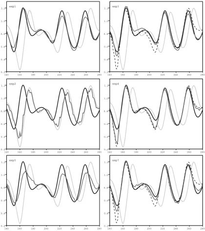
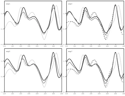
Fig. 4. Examples of assimilation for six relevant experiments described in Tab. 1. The only difference between the panels on the same line is
that translation is (resp. not) applied on the right (resp. left). The nature state (solid black curve) and the background (solid light grey curve) are the same in each panel. The translated background is the dashed curve when relevant (left panels). The results of assimilation are plotted in solid dark grey.
Fig. 4. Examples of assimilation for six relevant experiments described in Table 1. The only difference between the panels on the same line is
that translation is (resp. not) applied on the right (resp. left). The nature state (solid black curve) and the background (solid light grey curve) are the same in each panel. The translated background is the dashed curve when relevant (right panels). The results of assimilation are plotted in solid dark grey.
The main issue is how to compute the typical position er-ror σt of background coherent structures (that leads to the
parameterw1) and the background covariance matrix B0. A
common formulation of background error covariance is from Derber and Bouttier (1999), in which cross-parameter corre-lations are expressed from vorticity. Covariances are com-puted from an ensemble of coupled forecasts valid at the same instant. For every forecast, two-dimensional coherent
structures at every model level are identified in the rela-tive vorticity using the above-mentioned algorithm. The typ-ical position error σt of coherent structures at every level
Fig. 5. Other examples of assimilation for four relevant experiments described in Tab. 1. Same legend as Fig. 4
The main issue is how to compute the typical position er-450
rorσtof background coherent structures (that leads to the
parameterw1) and the background covariance matrixB′. A common formulation of background error covariance is from Derber and Bouttier (1999), in which cross-parameter corre-lations are expressed from vorticity. Covariances are com-455
puted from an ensemble of coupled forecasts valid at the same instant. For every forecast, two-dimensional coherent structures at every model level are identified in the relative vorticity using the above-mentionned algorithm. The typ-ical position errorσt of coherent structures at every level
460
would be obtained by the distribution of the difference of positions of detected structures in the coupled forecasts. For each coupled forecast, its coherent structures in the vorticity field would be translated towards the corresponding coher-ent structures in the other forecast. At each level, the result-465
ing translations would be applied to every field in the same forecast, and the resulting covariances between the translated
forecast and the other one would lead to theB′matrix. It is expected that this method would change horizontal and ver-tical correlations but it would preserve cross-parameter cor-470
relations.
Using these statistics and the algorithm for identification of coherent structures, step 1 and step 2 would apply to any background. One of the advantage of background transla-tion is that the selectransla-tion of observatransla-tions to be assimilated 475
would be improved. Since such a procedure relies on keep-ing the observations that do not depart too much from the background, good observations would have a better chance if they are compared to the translated background.
5 Conclusions
480
A method to translate and assimilate coherent structures in the context of variational data assimilation has been
intro-Fig. 5. Other examples of assimilation for four relevant experiments described in Table 1. Same legend as intro-Fig. 4.
translations would be applied to every field in the same fore-cast, and the resulting covariances between the translated forecast and the other one would lead to the B0matrix. It is expected that this method would change horizontal and ver-tical correlations, but would preserve cross-parameter corre-lations.
Using these statistics and the algorithm for identification of coherent structures, step 1 and step 2 would apply to any background. One of the advantages of background transla-tion is that the selectransla-tion of observatransla-tions to be assimilated would be improved. Since such a procedure relies on keeping the observations that do not depart too much from the back-ground, good observations would have a better chance if they are compared to the translated background.
5 Conclusions
A method to translate and assimilate coherent structures in the context of variational data assimilation has been intro-duced. Application to the more general problem of fusion of geophysical data is also promising in the case of a data source that is prone to phase error. A simple and robust two-step algorithm is provided to compute the translation
field and the analysis. Validation of the method is provided in a one-dimensional system, but extension of the method to three-dimensional geophysical fields and even to a four-dimensional context (4D-Var) is possible. Application to a model vector state in the wavelet domain may be highly valu-able, since wavelet space is compatible with the representa-tion of coherent structures (Plu et al., 2008). Moreover, some studies have shown the advantage of formulating data assim-ilation in a wavelet space (Deckmyn and Berre, 2005).
Acknowledgements. This work was supported by the Fondation
MAIF under the PRECYP grant. I thank O. Talagrand, E. Blayo and two anonymous reviewers for their insightful remarks, and Marie-Dominique Leroux for a careful proofreading.
Edited by: O. Talagrand
Reviewed by: E. Blayo and two anonymous referees
The publication of this article is financed by CNRS-INSU.
References
Beezley, J. D. and Mandel, J.: Morphing ensemble Kalman filters, Tellus, 60A, 131–140, 2008.
Chen, Y. and Snyder, C.: Assimilating vortex position with an ensemble Kalman filter, Mon. Weather Rev., 135, 1828–1845, 2007.
Deckmyn, A. and Berre, L.: A wavelet approach to representing background error covariances in a limited-area model, Mon. Weather Rev., 133, 1279–1294, 2005.
Derber, J. and Bouttier, F.: A reformulation of the background er-ror covariance in the ECMWF global data assimilation system, Tellus, 51A, 195–222, 1999.
Gilbert, J. C. and Lemaréchal, C.: Some numerical experiments with variable-storage quasi-Newton algorithms, Math. Pro-gramm., 45, 407–435, 1989.
Heming, J. T., Chan, J. C., and Radford, A. M.: A new scheme for the initialisation of tropical cyclones in the UK Meteorological Office global model, Meteor. Appl., 2, 171–184, 1995.
Hoffman, R. N., Liu, Z., Louis, J.-F., and Grassoti, C.: Distortion representation of forecast errors, Mon. Weather Rev., 123, 2758– 2770, 1995.
Kalman, R. E.: A new approach to linear filtering and prediction problems, J. Basic Eng., 82D, 35–45, 1960.
Le Dimet, F.-X. and Talagrand, O.: Variational algorithm for anal-ysis and assimilation of meteorological observations: theoretical aspects, Tellus, 38A, 97–110, 1986.
Michel, Y.: Displacing potential vorticity structures by the assimila-tion of pseudo-observaassimila-tions, Mon. Weather Rev., 139, 549–565, 2011.
Montroty, R., Rabier, F., Westrelin, S., Faure, G., and Viltard, N.: Impact of wind bogus and cloud and rain affected SSM/I data on tropical cyclones analyses and forecasts, Q. J. R. Meteorol. Soc., 134, 1673–1699, 2008.
Parrish, D. F. and Derber, J. C.: The National Meteorological Center’s spectral statistical interpolation analysis system, Mon. Weather Rev., 120, 1747–1763, 1992.
Pereira, M. B. and Berre, L.: The use of an ensemble approach to study the background error covariances in a global NWP model, Mon. Weather Rev., 134, 2466–2489, 2006.
Plu, M., Arbogast, P., and Joly, A.: A wavelet representation of synoptic-scale coherent structures, J. Atmos. Sci., 65, 3116– 3138, 2008.
Ravela, S., Emanuel, K., and McLaughlin, D.: Data assimilation by field alignment, Physica D, 230, 127–145, 2007.
Talagrand, O.: Assimilation of observations, an introduction, J. Me-teor. Soc. Japan, 75, 191–209, 1997.
Talagrand, O. and Courtier, P.: Variational assimilation of meteoro-logical observations with the adjoint vorticity equation, I: The-ory, Q. J. R. Meteorol. Soc., 113, 1311–1328, 1987.
Titaud, O., Vidard, A., Souopgui, I., and Le Dimet, F.-X.: Assimi-lation of image sequences in numerical models, Tellus, 62A, 30– 47, 2010.