Using
Repetitive Sampling Scheme
Nasrullah Khan
Department of Statistics
University of Veterinary & Animal Sciences, Lahore (Sub Campus, Jhang), Pakistan
Muhammad Aslam
Department of Statistics
Faculty of Science, King Abdulaziz University, Jeddah 21551, Saudi Arabia [email protected]
Liaquat Ahmad
Department of Statistics
University of Veterinary & Animal Sciences, Lahore, Pakistan [email protected]
Chi-Hyuck Jun
Department of Industrial and Management Engineering POSTECH, Pohang, Republic of Korea
Abstract
In this manuscript, a control chart is designed when the quality characteristic of interest follows a gamma distribution using repetitive sampling. The Wilson-Hilferty approximation is used to transform the gamma distributed characteristic to a normal random variable. Two pairs of control limits are established and their control constants are determined by considering the specified in-control average run length (ARL). The out-of-control ARL is derived when the process is shifted in terms of the scale parameter of the Gamma distribution. The ARLs are presented for various values of the shape parameter according to process shift parameters. A simulated example is given to illustrate the proposed control chart.
Keywords: Wilson-Hilferty transformation, Gamma distribution, Normal distribution Control chart.
1. Introduction
and measurements from the accelerated life test are skewed in nature Derya and Canan
(2012). More details about the application and designing of control charts for non-normal distributions can be seen in Nelson (1979), Bai and Choi (1995) and Choobineh and
Ballard (1987).
Recently, Santiago and Smith (2013) proposed the control chart called a t-chart when the time between events follows the exponential distribution. They used the variable transformation proposed by Nelson (1994) to transform the exponential distributed data to an approximate normal data. Aslam et al. (2014) proposed a new control chart for the exponential distribution using the transformed variable and repetitive sampling. More details about this type of control charts and applications in variety of fields can be found
Das (1955), Stephenson (1966), Ashkar and Bobée (1988), Aksoy (2000), Bhaumik
and Gibbons (2006), Borror et al. (2003), Zhang et al. (2007), Dogu (2014).
The gamma distribution has been widely used in a variety of fields. This distribution is considered as a good fit for the waiting time data in life testing. Das (1955) and Stephenson (1966) discussed the application of a gamma distribution to model the rain fall data. Ashkar and Bobée (1988) and Aksoy (2000) presented the applications of this distribution in hydrological data. According to Bhaumik and Gibbons (2006), the two-parameter gamma distribution can be used in environment monitoring and control issues. More details about the applications of gamma distributions can be found in Borror et al. (2003). Zhang et al. (2007) proposed a random-shift model to measure the average run length for a gamma distribution. Recently, Dogu (2014) designed the control chart for a gamma distribution using several change point models.
The control charts available in the literature are designed using the single sampling scheme. Sherman (1965) introduced the repetitive sampling scheme in the area of acceptance sampling plan. Later on, Balamurali and Jun (2006) proved that an acceptance sampling plan using repetitive sampling is more efficient than single and double sampling in term of the average sample number. The designing of control charts for various situations using the repetitive sampling scheme has received the attention these days. Moreover, the repetitive sampling scheme is more efficient than the single sampling scheme in terms of reducing the average run length. The repetitive sampling is operated as follows: a random sample is selected from the production process and information about quality of interest is studied. A decision whether the process is in-control or out-of control is taken on the basis of sample information. Sometimes, it may happen that the decision cannot be reached on the basis of first sample from the production process. In this case, a new sample is selected from the production process and repeated until a decision is reached, see Sherman (1965). This sampling scheme is simple to operate as compared to double and sequential sampling.
t-charts using various sampling schemes can be seen in Lio et al. (2014), Aslam et al. (2015a, b, c, d), Azam et al. (2015).
Krishnamoorthy et al. (2008) presented an extensive study of various approximations for a gamma distribution. According to Krishnamoorthy et al. (2008), the Wilson-Hilferty (WH) (1931) approximation is a simple, satisfactory and unified approach for addressing various issues for the gamma distribution. According to the best of our knowledge, there is no work on designing the control chart for the gamma distribution using WH approximation. In this paper, we will design a control chart using repetitive sampling by assuming that the quality characteristic of interest follows the gamma distribution. We will use the WH approximation to transform the gamma distributed variable to a normal random variable and to set up the upper and the lower control limits. The control constant of the proposed control chart is determined for a specified in-control average run length (ARL). The out-of-control ARL is derived when the process is shifted in terms of the scale parameter. A simulation example will be given for the illustration purpose.
2. Proposed control chart for Gamma distribution
Let T be a random variable from a gamma distribution with shape parameter and scale parameter . The cumulative distribution function (cdf) of the gamma distribution is given by
( ) ∑ ( ⁄ ) (1)
The Wilson and Hilferty (1931) suggested that the transformation of is distributed approximately as normal with mean
( )
( ) (2)
and variance
( )
( ) (3)
This suggests that is symmetric in distribution, so a control chart can be designed with the usual symmetric type of control limits. Therefore, we propose the following control chart using repetitive sampling for a gamma distributed quality characteristic:
Step 1: Select an item randomly and measure its quality characteristic T. Then, calculate
⁄
(4)
Step 2: Declare the process as out-of-control if or . Declare the process as in-control if . Otherwise, go to Step 1 and repeat the process.
The proposed chart reduces to Aslam et al. (2014) chart when (an exponential case). The proposed chart reduces to the chart by Santiago and Smith (2013) when
and . It is assumed here that the control limits have the following forms and that they are constructed from the data when the process is in control. Let be the scale parameter when the process is in control. Then, the outer control limits are given by
⁄ ( )( ) √ ⁄ ( )
( ) (5a)
⁄ ( )( ) √ ⁄ ( )
( ) (5b)
The inner control limits are given by
⁄ ( )( ) √ ⁄ ( )
( ) (6a)
⁄ ( )( ) √ ⁄ ( )
( ) (6b)
The control coefficients and are to be determined by considering the specified in-control ARL.
Define
[ ( )
( ) √
( )
( ) (
( )
( ) ) ]
[ ( )
( ) √
( )
( ) (
( )
( ) ) ]
[ ( )
( ) √
( )
( ) (
( )
( ) ) ]
[ ( )
( ) √
( )
( ) (
( )
Then, the control limits in Eqs (5) and (6) are reduced to
⁄
⁄
⁄
⁄
Note that , , and do not depend on the scale parameter .
It is assumed that only the scale parameter of the gamma distribution will be changed when the process shift occurs. That is, the shape parameter remains unchanged even when the process is shifted. The shape parameter is usually differently fixed depending on a particular type of application similarly to the Weibull case Jun et al. (2006). Let be the scale parameter when the process is in control and let be the scale parameter when the process is shifted. Further, the scale parameter for the shifted process has the form of for a constant c.
Under the proposed control chart, the probability that the process is declared as out of control for a single sample is given by below when the process is actually in control.
( ) ( ) (7)
or
∑ ( )
∑
( )
(8)
The probability of repetition ( ) for the proposed control chart is given as follows
* + * + (9)
or
∑
( )
∑
( )
∑
( )
∑
( )
(10)
It should be noted that the control limits, and only depend on shape parameter which is assumed to be known in this study. The shape parameter can be estimated from the data when it is unknown. It should also be noted that the above probabilities are exact under the gamma distribution instead of a normal approximation. The normal approximation is utilized only when establishing the symmetric control limits. The probability of declaring as out-of- control under repetitive sampling is given as
The average run length (ARL) for the in-control process is given as follows:
(12)
Now, we assume that the scale parameter of the gamma distribution is changed from to , for a constant c. The probability of declaring as out- of- control for the shifted process based on a single sample is given as follows
( ) ( )
∑
( )
∑
( )
(13)
The probability of repetition under repetitive sampling is given as follows
* + * +
∑
( )
∑
( )
∑
( )
∑
( )
(14)
Therefore, the probability of declaring as out-of control for the shifted process is given as
(15)
The out-of-control ARL for the shifted process is given as follows
(16)
Table 1: The values of when
c
3.053036 3.267858 4.427538 8.199072 8.006176
0.332165 2.681024 3.781105 3.794553 4.078875
1.00 200.59 200.02 200.66 200.38 200.20
1.01 187.28 187.24 183.19 138.24 142.82
1.02 175.08 175.52 167.58 96.15 102.62
1.03 163.87 164.74 153.59 67.42 74.28
1.04 153.57 154.81 141.04 47.68 54.16
1.05 144.09 145.66 129.75 34.02 39.79
1.10 106.51 109.27 87.69 7.40 9.72
1.15 80.73 84.11 61.56 2.43 3.22
1.20 62.57 66.21 44.67 1.36 1.63
1.30 39.78 43.42 25.57 1.03 1.07
1.40 26.96 30.30 16.03 1.00 1.01
1.50 19.24 22.23 10.81 1.00 1.00
1.60 14.34 16.97 7.74 1.00 1.00
1.70 11.09 13.40 5.83 1.00 1.00
1.80 8.84 10.88 4.57 1.00 1.00
1.90 7.24 9.05 3.72 1.00 1.00
2.00 6.07 7.67 3.12 1.00 1.00
2.50 3.24 4.19 1.78 1.00 1.00
3.00 2.25 2.88 1.37 1.00 1.00
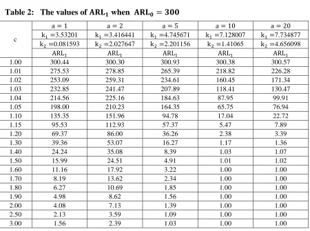
Table 2: The values of when
c
3.53201 3.416441 4.745671 7.128007 7.734877
0.081593 2.027647 2.201156 1.41065 4.656098
1.00 300.44 300.30 300.93 300.38 300.57
1.01 275.53 278.85 265.39 218.82 226.28
1.02 253.09 259.31 234.61 160.45 171.34
1.03 232.85 241.47 207.89 118.41 130.47
1.04 214.56 225.16 184.63 87.95 99.91
1.05 198.00 210.23 164.35 65.75 76.94
1.10 135.35 151.96 94.78 17.04 22.72
1.15 95.53 112.93 57.37 5.47 7.89
1.20 69.37 86.00 36.26 2.38 3.39
1.30 39.36 53.07 16.27 1.17 1.36
1.40 24.24 35.08 8.39 1.03 1.07
1.50 15.99 24.51 4.91 1.01 1.02
1.60 11.16 17.92 3.22 1.00 1.00
1.70 8.19 13.62 2.34 1.00 1.00
1.80 6.27 10.69 1.85 1.00 1.00
1.90 4.98 8.62 1.56 1.00 1.00
2.00 4.08 7.13 1.39 1.00 1.00
2.50 2.13 3.59 1.09 1.00 1.00
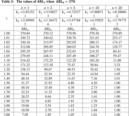
Table 3: The values of when
c
2.82152 1
3.54827 3
4.72527 4
5.80871 1
8.28060 4 2.69969
2
1.36472 6
2.47768 1
4.35825 1
3.79775 3
1.00 370.84 370.12 370.96 370.38 370.89
1.01 349.72 340.62 328.76 321.63 253.17
1.02 330.18 313.97 292.05 280.13 174.17
1.03 312.08 289.85 260.03 244.70 120.77
1.04 295.29 267.97 232.03 214.35 84.41
1.05 279.69 248.11 207.49 188.27 59.47
1.10 216.42 172.25 122.29 102.26 11.88
1.15 171.22 123.30 75.47 58.84 3.33
1.20 138.12 90.67 48.53 35.62 1.56
1.30 94.44 52.54 22.35 14.94 1.05
1.40 68.16 32.89 11.67 7.36 1.01
1.50 51.37 21.92 6.80 4.20 1.00
1.60 40.10 15.40 4.38 2.73 1.00
1.70 32.23 11.32 3.09 2.00 1.00
1.80 26.53 8.64 2.35 1.61 1.00
1.90 22.29 6.82 1.91 1.39 1.00
2.00 19.06 5.54 1.63 1.25 1.00
2.50 10.50 2.70 1.15 1.04 1.00
3.00 7.05 1.85 1.05 1.01 1.00
From Tables 1-3, we note the following trend:
1. For the same values of , decreases as increases.
2. There is no specific trend in value of k as the shape parameter increases.
3. decreases rapidly as value of increases.
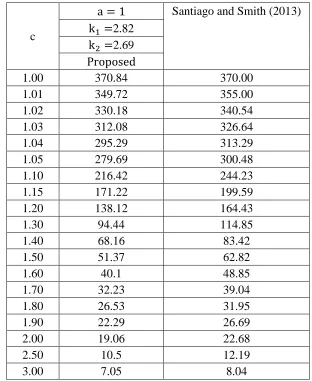
3. Advantages of the Proposed Chart
various values as compared to existing control chart. For example, when = 370 and = 1.1, the proposed control provides =216, while it is 244 from the chart by proposed by Santiago and Smith (2013). So, the proposed control chart performs better than control charts proposed by Santiago and Smith (2013) in terms of detecting early shift in the manufacturing process.
Table 4: Comparison of Proposed Chart with Santiago and Smith (2013) charts when
c
Santiago and Smith (2013)
2.82 2.69
1.00 370.84 370.00
1.01 349.72 355.00
1.02 330.18 340.54
1.03 312.08 326.64
1.04 295.29 313.29
1.05 279.69 300.48
1.10 216.42 244.23
1.15 171.22 199.59
1.20 138.12 164.43
1.30 94.44 114.85
1.40 68.16 83.42
1.50 51.37 62.82
1.60 40.1 48.85
1.70 32.23 39.04
1.80 26.53 31.95
1.90 22.29 26.69
2.00 19.06 22.68
2.50 10.5 12.19
3.00 7.05 8.04
The efficiency of proposed chart is also compared with existing control chart for the gamma distribution. Again, the values of are placed in Table 5 for both control charts for same values of specified parameters. From Table 5, we note that the proposed chart performs better than existing control chart for gamma distribution at all values of shifts. For example, when =370, and =1.1, the proposed control provides
Table 5: Comparison of Proposed Chart with existing gamma charts when
c
Existing chart when
4.72
2.47
1.00 370.96 370.00 1.01 328.76 344.44 1.02 292.05 321.12 1.03 260.03 299.81 1.04 232.03 280.30 1.05 207.49 262.42 1.10 122.29 192.35
1.15 75.47 145.07
1.20 48.53 112.18
1.30 22.35 71.42
1.40 11.67 48.71
1.50 6.80 35.07
1.60 4.38 26.39
1.70 3.09 20.59
1.80 2.35 16.55
1.90 1.91 13.64
2.00 1.63 11.48
2.50 1.15 6.07
3.00 1.05 4.05
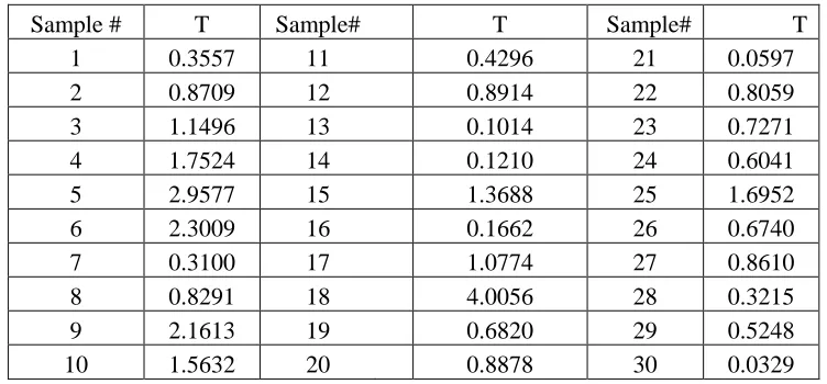
4. Simulation Study
Now, we will discuss the application of the proposed control chart using the simulated data. First 30 observations of the data is generated from the gamma distribution assuming that process is in control when . Let = 370. Next 35 observations are generated from the gamma distribution by assuming that process has shifted to ( =1.7). The data of 30 observations is reported in Table 6.
Table 6: Data of 30 observations from a gamma distribution
Sample # T Sample# T Sample# T
1 0.3557 11 0.4296 21 0.0597
2 0.8709 12 0.8914 22 0.8059
3 1.1496 13 0.1014 23 0.7271
4 1.7524 14 0.1210 24 0.6041
5 2.9577 15 1.3688 25 1.6952
6 2.3009 16 0.1662 26 0.6740
The transformed data ⁄ is given in Table 7.
Table 7: Transformed data using transformation
Sample # Sample# Sample#
1 0.7086 11 0.7545 21 0.3910
2 0.9549 12 0.9624 22 0.9306
3 1.0475 13 0.4663 23 0.8992
4 1.2056 14 0.4946 24 0.8453
5 1.4354 15 1.1103 25 1.1923
6 1.3201 16 0.5498 26 0.8767
7 0.6768 17 1.0251 27 0.9513
8 0.9394 18 1.5881 28 0.6850
9 1.2929 19 0.8802 29 0.8066
10 1.1605 20 0.9611 30 0.3207
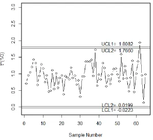
The four limits are obtained by =-0.0223, =0.0199, =1.7660 and
=1.8082. We plotted the transformed data ⁄ on the control chart in Figure 1.
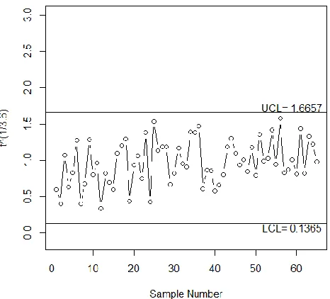
From this control chart, we can see that the proposed chart detects the shift at 32th observation. We also plotted 30 values on control chart by Santiago and Smith (2013) in Figure 2.
Figure 2: Existing chart for the simulated data
From Fig. 2, we note that the control chart by Santiago and Smith (2013) does not detect the shift. So, the proposed chart has ability to detect the shift in the process earlier as compared to the existing control chart.
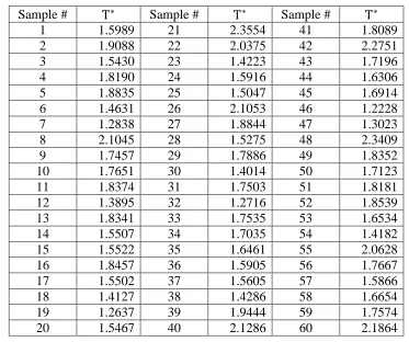
5. Application of Proposed Chart
By plotting the statistic on control chart in Figure 3, it can be seen that several values of are near to and and two values lie in repetitive area. The Figure 3, clearly indicates that cause of variation in the process should be indicated.
Table 8: The UTIs data
Sample # Sample # Sample #
1 1.5989 21 2.3554 41 1.8089
2 1.9088 22 2.0375 42 2.2751
3 1.5430 23 1.4223 43 1.7196
4 1.8190 24 1.5916 44 1.6306
5 1.8835 25 1.5047 45 1.6914
6 1.4631 26 2.1053 46 1.2228
7 1.2838 27 1.8844 47 1.3023
8 2.1045 28 1.5275 48 2.3409
9 1.7457 29 1.7886 49 1.8352
10 1.7651 30 1.4014 50 1.7123
11 1.8374 31 1.7503 51 1.8181
12 1.3895 32 1.2716 52 1.8539
13 1.8341 33 1.7535 53 1.6534
14 1.5507 34 1.7035 54 1.4182
15 1.5522 35 1.6461 55 2.0628
16 1.8457 36 1.5905 56 1.7667
17 1.5502 37 1.5605 57 1.5866
18 1.4127 38 1.4286 58 1.6654
19 1.2637 39 1.9444 59 1.7574
20 1.5467 40 2.1286 60 2.1864
6. Concluding Remarks
We proposed a new control chart for the gamma distribution. The WH transformation is used to establish the symmetric control limits of the proposed control chart. Tables are provided for practical use and comparison is made with the existing control chart. The proposed control chart is found to outperform the control chart proposed by Santiago and Smith (2013) and Aslam et al. (2014). The application of the proposed control chart is given with the help of a simulated data. The proposed control chart can be used in the industry for the manufacturing process when the time between events follows the exponential distribution or gamma distribution with known or unknown shape parameter. The proposed control chart will be extended using the other sampling schemes as a future research.
Acknowledgements
Jeddah. The author, Muhammad Aslam, therefore, acknowledge with thanks DSR technical and financial support.
References
1. Chase, N. (1997). SPC provides 1000% ROI. Quality, 36, 62-63.
2. Derya, K. and Canan, H. (2012). Control Charts for Skewed Distributions: Weibull, Gamma, and Lognormal. Advances in Methodology & Statistics/Metodoloski zvezki, 9(2), 95-106.
3. Nelson, P.R. (1979). Control charts for Weibull processes with standards given. Reliability, IEEE Transactions, 28(4), 283-288.
4. Bai, D. and Choi, I. (1995). (X) OVER-BAR-CONTROL AND R-CONTROL CHARTS FOR SKEWED POPULATIONS, Journal of Quality Technology,. 27(2), 120-131.
5. Choobineh, F. and Ballard, J. (1987). Control-limits of QC Charts for skewed distributions using weighted-variance, Reliability, IEEE Transactions, 36(4), 473-477.
6. Santiago, E. and Smith, J. (2013). Control charts based on the exponential distribution: Adapting runs rules for the t chart, Quality Engineering, 25(2), 85-96.
7. Nelson, L.S. (1994). A control chart for parts-per-million nonconforming items, Journal of Quality Technology, 26(3), 239-240.
8. Aslam, M., Khan, N., Azam, M., and Jun, C. H. (2014). Designing of a new monitoring t-chart using repetitive sampling. Information Sciences, 269, 210-216.
9. Das, S. (1955). The fitting of truncated type III curves to daily rainfall data, Australian Journal of Physics, 8(2), 298-304.
10. Stephenson, D. B., Kumar, K. R., Doblas-Reyes, F. J., Royer, J. F., Chauvin, F., and Pezzulli, S. (1999). Extreme daily rainfall events and their impact on ensemble forecasts of the Indian monsoon. Monthly Weather Review, 127(9), 1954-1966.
11. Ashkar, F., and Bobée, B. (1988). Confidence intervals for flood events under a Pearson 3 or log Pearson 3 distribution. Water Resources Bulletin, 24(3), 639-650.
12. Aksoy, H. (2000). Use of gamma distribution in hydrological analysis. Turkish Journal of Engineering and Environmental Sciences, 24(6), 419-428.
13. Bhaumik, D.K. and Gibbons, R.D. (2006). One-sided approximate prediction intervals for at least p of m observations from a gamma population at each of r locations, Technometrics, 48(1), 112-119.
16. Dogu, E. (2014). Change point estimation based statistical monitoring with variable time between events (TBE) control charts. Quality Technology & Quantitative Management, 11(4), 383-400.
17. Sherman, R.E.(1965). Design and evaluation of a repetitive group sampling plan. Technometrics, 7(1), 11-21.
18. Balamurali, S. and Jun, C.-h. (2006). Repetitive group sampling procedure for variables inspection, Journal of Applied Statistics, 33(3), 327-338.
19. Aslam, M., Azam, M., and Jun, C. H. (2014). New attributes and variables control charts under repetitive sampling. Industrial Engineering & Management Systems, 13(1), 101-106.
20. Ahmad, L., Aslam, M., and Jun, C.-H. (2014). Designing of X-bar control charts based on process capability index using repetitive sampling. Transactions of the Institute of Measurement and Control, 36(3), 367-374.
21. Aslam, M., Azam, M., and Jun, C. H. (2014). A new exponentially weighted moving average sign chart using repetitive sampling. Journal of Process Control, 24(7), 1149-1153.
22. Lio, Y. L., Tsai, T. R., Aslam, M., and Jiang, N. (2014). Control charts for monitoring Burr type-X percentiles. Communications in Statistics-Simulation and Computation, 43(4), 761-776.
23. Aslam, M., Azam, M. Jun, C.-H. (2015a). A New Control Chart for Exponential Distributed Life Using EWMA, Transactions of the Institute of Measurement and Control, 37(2), 205-210.
24. Aslam, M., Azam, M., Khan, N. Jun, C.-H. (2015b). A Control Chart for an Exponential Distribution Using Multiple Dependent State Sampling, Quality and Quantity, 49, 455-462.
25. Aslam, M., Nazir, A. Jun, C.-H. (2015c). A New Attribute Control Chart using Multiple Dependent State Sampling, Transactions of the Institute of Measurement and Control, 37 (4), 569-576.
26. Azam, M., Aslam, M. and Jun, C.-H. (2015). Designing of a hybrid exponentially weighted moving average control chart using repetitive sampling, International Journal of Advanced Manufacturing Technology, 77, 1927–1933.
27. Aslam, M. and Jun, C.-H. (2015d). Attribute Control Charts for the Weibull Distribution under Truncated Life Tests, Quality Engineering, 27, 283-288.
28. Krishnamoorthy, K., Mathew, T., and Mukherjee, S. (2012). Normal-based methods for a gamma distribution. Technometrics.
29. Wilson, E. B., and Hilferty, M. M. (1931). The Distribution of Chi-Squares,” Proceedings of the National Academy of Sciences, 17, 684–688.