Closed form solution of an exponential kernel integral equation

Closed Form Solution of an Exponential Kernel Integral Equation

Wynand Verwoerd, Senior Lecturer, Center for Advanced Computational Solutions, Lincoln University, New Zealand, [email protected]

Abstract

In this note a Fredholm integral equation of the first kind with exponential expressions for the kernel and right hand side is considered. The task of finding a practically usable solution to such an equation may need more effort than following a standard procedure, even when such a procedure yields a formal solution. An apparently elegant solution as an orthogonal polynomial expansion is obtained using the standard method based on transformation to a form where the kernel is an orthogonal polynomial generating function, but this is of limited use due to slow convergence. It is shown that this can nevertheless be transformed into a closed form solution that is computationally efficient.

2000 Mathematics Subject Classification: 41A10, 45H05, 76S05

The definitive version is available at

http://www.scientificjournals.org/journals2007/articles/1231.pdf

1. Introduction

The fact that a solution to a differential or integral equation can be found by standard general purpose methods, is no guarantee that this solution will be practically usable e.g. for

numerical calculations. This is true even when a solution in a closed functional form that can be readily calculated, does exist. The formal solution method will not necessarily find this solution. So the task of solving the equation does not end with the formal solution, but extends to looking for an alternative functional form that can be computed efficiently.

The situation is demonstrated in this note for the following Fredholm integral equation of the first kind:

(

)

2 2 2

( , , )

a x

exp

1

z

2

z

F x y z e

dx

a

e

a y e

∞ ₋

−∞

−

⎡

⎤

=

_⎣

−

+

_⎦

∫

(1)

where the function F(x,y,z) is to be found with a,x,y,z∈R and z ≥ 0.

Integral equations with this structure were encountered in the context of a stochastic differential equation model of solute transport in a porous medium (Kulasiri & Verwoerd, 2002), where use of the solution in further mathematical development of the theory required a closed form of the solution rather than a formal series expansion.

2. Formal Solution

Equation (1) is transformed into a more amenable form by the following substitution:

(2)

2 2

( , , )

y x

( , , )

F x y z

=

e

−

G x y z

Substituting this into equation (1) yields an integral equation for G(x,y,z)

(

)

2 2

( )

( , , )

a x

( ) exp

z

G x y z e

dx

g a

a e

y

∞ _{− − −}

−∞

⎡

⎤

=

≡

_⎢

−

−

_⎥

⎣

⎦

In this equation, the kernel is the generating function for Hermite polynomials Hn(a) (Hochstrasser, 1965) 2 2 ( ) 0

( )

!

a

a x n

n n

e

e

H

n

− ∞ − − =

=

∑

a x

(4)

As shown in (Morse & Feshbach, 1953) substituting this and employing the orthonormalization of the polynomials yields the solution

( ) 0

1

(0)

( , , )

( )

2 !

n n n n

g

G x y z

H x

n

π

∞

=

=

∑

(5)

From the Rodrigues’ formula (Hochstrasser, 1965) for the n-th Hermite polynomial

2

( ) ( 1)

n

n z z

n n

d

H z

e

e

dz

2

−

= −

(6)

it follows that

(

)

2

( )n

_{( )}

n z

_{( 1) exp}

n z

₍

z

₎

n

g

a

=

e

−

−

_⎢

⎡

−

a e

−

−

y

⎤

_⎥

H a e

−

y

⎣

⎦

−

(7)

and hence the solutions of equations (3) and (1) are respectively given by

2

0

( , , )

( )

( )

!2

y n z

n n

n n

e

e

G x y z

H

x H

y

n

π

− ∞ −

=

=

∑

(8)

2

0

( , , )

( )

( )

!2

x n z

n n

n n

e

e

F x y z

H

x H

y

n

π

− ∞ −

=

=

∑

(9)

While the standard method yields formal solutions to the integral equations, they are not useful in numerical computation because of the poor convergence of the bilinear Hermite series common to (8) and (9).

The formal convergence of the series is easily proven for z≥0 by using the inequality (Hochstrasser, 1965)

2 1 2

( )

x

!2

n n

H x

<

k e

n

(10)

where k is a number of order 1.

Nevertheless numerical convergence is slow. That is demonstrated by plotting partial sums of the series factor common to both solutions

0

( , , )

( )

( )

!2

n z N

N n n

n

e

S

x y z

H x H

y

n

−

=

Figure 1 shows this for increasing N values, as a function of x for arbitrarily chosen values y = 1.5 and z = 2.5. It is seen that there is a central peak common to all three plots, but outside the extent of this peak the behaviour is numerically very unstable.

(a)

(b)

(c)

Figure 1: Partial sums SN(x,y,z) as function of x for y = 1.5, z = 2.5 and (a) N = 5 (b) N = 20 and (c) N =

50 . All three plots are drawn to the same scale.

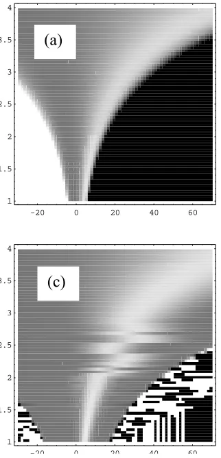
The convergence of the series depends sensitively on the value of z. An overview of this is shown in Figure 2. In the figure, the light coloured band that curves upwards and to the right represents the peak that was shown in Figure 1 as it evolves for increasing z-values. As more terms are included in the partial sum, the smoothly shaded grey area where the sum converges, expands, but only very slowly.

-20 0 20 40 60

1 1.5 2 2.5 3 3.5 4

-20 0 20 40 60

1 1.5 2 2.5 3 3.5 4

-20 0 20 40 60

1 1.5 2 2.5 3 3.5 4

(a)

(b)

(c)

Figure 2: Density plots of partial sums SN(x,y,z) with y = 1.5, -30≤x≤70 and 1≤ z≤ 4 for (a) N = 5

The convergence is worse for smaller z values as the sharpness of the central peak increases; in the limit z → 0 the infinite sum reduces to the completeness relation for Hermite polynomials (see equation (13) below) so that the peak approaches the Dirac delta function centered at x = y = 1.5 in this case. The ragged edge and the alternation between black and white areas (that represent large negative or positive values respectively) outside of the smoothly shaded peak are both indications of numerical instability.

Even with only 5 terms in the expansion, substituting in the explicit forms of the Hermite polynomials will obviously already result in a very complicated formula for the approximate solution. Applying computing technology allows one to ignore this; but even with as many as 500 terms in the expansion, there remain substantial ranges of x and z where the partial sum still behaves erratically. In fact the figure shows that this problem becomes even worse as N

increases, although the stability region of the partial sum approximation does expand (albeit at a disappointingly slow rate).

3. Closed form solutions

Having reached a formal solution, there is no general recipe for transforming this into a more amenable form and it is hard even to know if such a form exists. Symbolic algebra software may be helpful in simple cases but for this example did not lead to simplification of the result. However, a literature search led to a relatively obscure result known as the Mehler formula (Srivastava & Manocha, 1984), that contains bilinear sums of Hermite polynomials:

( )

₁

(

₂

)

1 2

(

2 2

)

2

2 2

0

2

( )

( )

1

exp

!

1

n

n n

n

x y w

x

y

w

H x H

y

w

w

n

w

∞ ₋

=

⎛

₋

₊

⎞

⎜

⎟

= −

⎜

−

⎟

⎝

⎠

∑

(12)

Putting w = e-zinto the left hand side of this formula reproduces , the infinite sum version of

( , , )

S

_∞

x y z

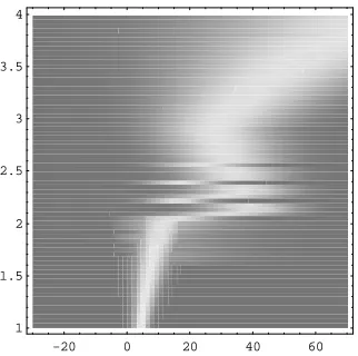
(11) that occurrs in equations (8) and (9). A plot of the right hand side closed expression in (12) gives the smooth behaviour demonstrated by Figure 3, and agrees with the partial sums inside their stability regions that was shown in Figure 2.

-20 0 20 40 60

1 1.5 2 2.5 3 3.5 4

Figure 3. Density plot of S(x,y,z) for y = 1.5, -30 ≤x≤ 70 and 1 ≤z≤ 4

The form of equation (12) shows that a real solution is obtained only for z>0. For z = 0 the sum can be evaluated directly from the completeness relation for parabolic cylinder functions (Abramowitz & Stegun, 1965) that are related to Hermite polynomials, which yields

2

0

( )

( )

(

)

!2

y

n n

n n

H x H

y

e

x

n

π δ

∞

=

=

Using these results, the solutions of equations (1) and (3) finally reduce to the closed forms

(

)

2

2 2

(

)

( , , )

1

exp

0

1

1

z

z z

x

y

z

x

y e

F x y z

z

e

e

δ

π

−

− −

0

−

=

⎧

⎪⎪

_⎛

₋

_⎞

= ⎨

_⎜

₋

_⎟

_>

⎪

₋

_⎜

₋

_⎟

⎪

_⎝

_⎠

⎩

(14)

(

)

2

2 2

(

)

( , , )

1

exp

0

1

1

z

z z

x

y

z

x e

y

G x y z

z

e

e

δ

π

−

− −

0

−

=

⎧

⎪⎪

_⎛

₋

_⎞

= ⎨

_⎜

₋

_⎟

_>

⎪

₋

_⎜

₋

_⎟

⎪

_⎝

_⎠

⎩

(15)

In addition to their computability, these functional forms give far more insight into how the arguments determine the behaviour of the solutions than the equivalent series expansions (8) and (9).

As is seen from this example, the generalised textbook recipes for solving differential and integral equations may need to be supplemented by ad hoc methods to obtain solutions in a form suitable for further numerical or analytic processing.

References

Abramowitz, M., & Stegun, I. A. (1965). Handbook of mathematical functions. New York: Dover Publications.

Hochstrasser, U. W. (1965). Orthogonal Polynomials. In M. Abramowitz, Stegun, Irene A. (Ed.), Handbook of Mathematical Functions (pp. 771-802). New York: Dover Publications.

Kulasiri, D., & Verwoerd, W. (2002). Stochastic dynamics - Modeling solute transport in porous media (Vol. 44). New York: Elsevier.

Morse, P. M., & Feshbach, H. (1953). Methods of theoretical physics. New York: McGraw-Hill. Srivastava, H. M., & Manocha, H. L. (1984). Treatise on Generating Functions. Chichester: