Estimating Continuous-Time Income Models
Christian Schluter
†and Mark Trede
‡18/2011
† Department of Economics, University of Southampton, UK ‡ Department of Economics, University of Münster, Germany
wissen
•leben
Estimating Continuous-Time Income Models
Christian Schluter
∗University of Southampton
Mark Trede
†Universität Münster
January 2011
Abstract: A fundamental component of inter-temporal consumption-saving and portfolio allo-cation models is a statistical model of the income process. While income processes are
com-monly unobservable income flows which evolve in continuous time, observable income data
are usually discrete, having been aggregated over time. We consider continuous-time earning
processes, specifically non-linearly transformed Ornstein-Uhlenbeck processes, and the
associ-ated integrassoci-ated, i.e. time aggregassoci-ated process. Both processes are characterized, and we show that time aggregation alters important statistical properties. The parameters of the earning
process are estimable by GMM, and the finite sample properties of the estimator are
investi-gated. Our methods are applied to annual earnings data for the US. It is demonstrated that the model replicates well important features of the earnings distribution.
Keywords: income processes, integrated non-linearly transformed Ornstein-Uhlenbeck process, temporal aggregation.
JEL classification: C22, E21, E24, J31
∗Department of Economics, University of Southampton, Highfield, Southampton, SO17 1BJ, UK.
Tel. +44 (0)2380 59 5909, Fax. +44 (0)2380 59 3858. Email: [email protected].
http://www.economics.soton.ac.uk/staff/schluter/
†Corresponding author. Center for Quantitative Economics and Center for Nonlinear Science, Westfälische
Wilhelms-Universität Münster, Am Stadtgraben 9, 48143 Münster, Tel.: +49-251-83 25006, Fax: +49-251-83 22012, Email: [email protected].
1
Introduction
A fundamental component of inter-temporal consumption-saving and portfolio allocation models is a statistical model of the income process (see e.g. the discussion in Wang (2009)). Assumed to
evolve in continuous time, popular modeling choices are variants of Brownian motion processes.1
The principal obstacle to the empirical implementation and the eventual testing of a model’s prediction, however, is the nature of the income data reported in the usual surveys: neither
is the income flow observable, nor is the income process sampled at specific time points; what
is reported in survey data is income data aggregated, by necessity, over time intervals. We address this problem by considering a statistical model of a continuous-time earnings process, and we propose methods to estimate its parameters from discretely sampled time-aggregated data. The estimation approach suggested in this paper therefore bridges the gap between the theoretical models and their empirical application. Moreover, we consider (Mincerian) classes of income processes, which are a more general than common modeling choices, and show that the estimated process describes well the US earnings distributions.
More specifically, we assume that the unobserved continuous-time earnings process is a
non-linearly transformed Ornstein-Uhlenbeck (OU) process. In the baseline model, the transforma-tion is an exponentiatransforma-tion, in the generalized model it is an inverted Box-Cox transformatransforma-tion. This process is sampled over possibly non-regular intervals, resulting for the baseline model in an integrated exponentiated Ornstein-Uhlenbeck process (intexpOU) and for the general model in an integrated inverted Box-Cox Ornstein-Uhlenbeck process (intinvBCOU). We characterize both expOU and intexpOU processes in terms of distributions and moments. In particular, we show that whereas the expOU process is Markov and lognormal, the intexpOU is neither. This
is an important finding since it demonstrates that wrongly assuming the observed integrated
process to have the same distributional properties as the unobservable underlying continuous-time process would introduce a temporal aggregation bias.
We demonstrate how the parameters of the unobservable income process are estimable from standard time-aggregated data by means of a GMM procedure. The merit of our approach is
illustrated using US PSID income data, and we show that the estimated modelfits the data very
well.
This is thefirst paper, to the best of our knowledge, to consider the estimation of
continuous-time earnings processes from continuous-time-aggregated data. The common approach in the labor
eco-1E.g. simple geometric Brownian motion (e.g. Bodie et al. (1992), Koo (1998), or Bick et al. (2009)), Brownian
motion with drift (Henderson, 2005), or geometric Brownian motion with time-varying drift and depending on other economic variables (Munk and Sørensen, 2009). Wang (2004, 2006, 2009) considers an Ornstein-Uhlenbeck process.
nomics literature is to estimate a discrete-time error component model on annual earnings data (e.g. MaCurdy, 1982, Abowd and Card, 1989, Baker, 1997, Guvenen, 2009). Integrated
diffu-sion processes are thus new to this empirical setting, but have been considered in other fields.
We highlight the principal differences. In the statistics literature, Gloter (2001) considers an integrated stationary Ornstein-Uhlenbeck process (intOU), which is shown to be Gaussian and
ARMA(1,1) with an exponentially decayingα-mixing coefficient. The likelihood is intractable
and he proposes a Whittle estimator for the OU parameters. However, his results do not apply to our case since the non-linear transform (exponentiation in the baseline model) prior to
inte-gration leads to completely different distributional properties of intexpOU and intOU processes.2
Such intOU processes are considered particularly infinance, and estimated for settings in which
the sampling time interval, required to be regular, converges to zero (e.g. Ditlevsen and Sørensen
(2004), or Gloter (2006)). The leading application is stochastic volatility modeling in finance
(e.g. Barndorff-Nielsen and Sheppard (2001)). In contrast to this literature our empirical setting does not allow to shrink the time interval to zero, nor do we require the time intervals to be
regular. Another strand of thefinance literature deals with integrated continuous-time processes
in the context of Asian option pricing (e.g. Carr and Schröder (2004)). Finally, turning to the consequences of temporal aggregation, such aggregation can, as in our case, lead to important differences between the continuous and the integrated process. Referring to such differences as time aggregation biases, these have been studied in a macro context in Harvey and Stock (1989) and Christiano, Eichenbaum and Marshall (1991), who consider how time-aggregation alters the results of tests of the permanent income hypothesis.
This paper is structured in the following way: In Section 2 we present the statistical model for the income process. Section 3 derives the moments of the time-aggregated, observable process. In Section 4 we suggest a more general non-linear transformation (Box Cox transformation)
for the income flow which permits the modeling of heavy tails. Section 5 sets out the GMM
estimation procedure. While the asymptotic properties of GMM are known to be attractive, not much can be said about its small sample properties. Therefore, in Section 6, we conduct
simulation exercises andfind that our estimation approach performs well even in relatively small
samples. Section 7 contains the empirical application in which we estimate the parameters of the continuous-time model using annual panel data from the US PSID. The model turns out to
fit the data very well. Section 8 concludes. All proofs are collected in the Appendix.
2Other related work includes Bhattacharya, Thomann and Waymire (2001), who derive partial differential
equations for the distribution of integrals of geometric Brownian motions. This is a special case of the intexpOU process if the mean reversion parameter of the OU process is absent. Comte, Genon-Catalot and Rozenholc (2009) suggest a nonparametric estimation method for integrated diffusions.
2
The Statistical Model for the Income Process
The log-incomeflow of an individual, denoted by {lnY (t) :t≥t0}, is assumed to follow a
sto-chastic process evolving in continuous time. t0 denotes the starting time of the process. We
impose a structure on this earnings process which follows conventional modeling, except that our
process evolves in continuous rather than discrete time. Specifically, we assume that the earnings
process decomposes additively into two independent parts. The error process is Gaussian and
denoted by{u(t) :t≥t0}, the model for the mean log-incomeflow is denoted by{y˜(t) :t≥t0},
and we assume that
lnY (t) = ˜y(t) +u(t). (1)
In Section 4 below we also consider more general Box-Cox transformations of theY (t)process.
The model for {y˜(t)} is standard in the sense of relating the mean log-income linearly to
observables such as measures of human capital. In our empirical application we postulate a Mincerian model. For notational convenience later, we partition the relevant observables into time-invariant and time-varying covariates
˜
y(t) =m+Z1>β+Z2>(t)γ. (2)
We treat the regressors as exogenous and follow e.g. Abowd and Card (1989) in ignoring the potential endogeneity of the human capital measure such as schooling which could arise from
unobserved ability. The interceptm, allowed to be individual-specific in order to accommodate
unobserved heterogeneity, is modelled as a random effect,
m=μ+ε,
withεhaving a zero-mean Gaussian distribution with varianceσ2ε.
The Gaussian latent variable or error process{u(t)}is assumed to be a zero-mean
Ornstein-Uhlenbeck (OU) process, governed by the stochastic differential equation
du(t) =−ηu(t)dt+σdW(t), (3) with solution u(t) =u(t0)e−ηt+σ Z t t0 eη(s−t)dW(s). (4)
{W(t) :t≥t0}is the standard Wiener process, andη∈Randσ >0are the parameters of the process.
The OU process is an attractive point of departure for two reasons. First, it is the continuous-time counterpart of an autoregressive process in discrete continuous-time. Autoregressive processes are commonly used for models of income dynamics in discrete time. Second, OU processes capture
not only stable processes but also unit root processes and, ifη <0, even explosive processes. In contrast to the common stability assumption, we do not impose any restrictions on the parameter
η.
The parameter σ determines the strength of the stochastic income component, and equals
the diffusion coefficient of the process. −ηu(t) is the instantaneous mean of the OU process.
The start value of the OU process u(t0) is assumed to be stochastic with E(u(t0)) = 0 and
V ar(u(t0)) =s20. Mean and covariances are given byE{u(t)}= 0and, forη6= 0,3
σs,t≡Cov(u(s), u(t)) = σ2 2ηe −η|t−s|+ae−η(t+s) (5) with a=s20−σ 2 2η (6)
for notational simplicity. Finally we note that the OU process is weakly stationary if a = 0,
i.e. s20=σ2η−1/2, and strongly stationary ifu(t0)is in addition Gaussian. However, we do not
impose any stationarity assumption.
Exponentiating the process (1) yields the continuous-time income process {Y (t) :t≥t0},
Y (t) = exp (˜y(t) +u(t)),
which is an exponentiated OU process (expOU).
A key assumption is that the econometrician cannot sample the process at specific points of
time. Instead, only the time-aggregated process is observable, i.e. the econometrician observes
the integrated process for non-overlapping time intervals[t0, t1], . . . ,[tT−1, tT]. Depending on the
specific application, these time intervals could be individual-specific if the data are spell data,
and common across individuals when the data are annual panel data. Below we refer to time
intervals that are common across individuals and of the same length∆as regular intervals. The
observable process is thus the integrated exponential Ornstein-Uhlenbeck (intexpOU) process
Sk= Z tk tk−1 Y(t)dt= Z tk tk−1 ey˜(t)eu(t)dt k= 1, . . . , T. (7) For ease of reference, we collect the model parameters in the vector
θ= [η, σ, s0, μ, σε, β, γ]>. (8)
We proceed to characterize both the unobservable income process {Y (t)} and the observable
integrated process{Sk}.4 In particular, important distributional properties of {Y(t)}will not
be inherited by{Sk}.
3We exclude the unit root case for expositional and notation ease by assumingη6= 0. However, all results can
be specialized forη→0.
4We follow notational convention and denote a continuous-time stochastic process byA(t)and an aggregated
3
Characterizing the Time Aggregated Process
Proposition 1 The unobservable income process{Y (t)}is lognormal and Markov, with E(Y(t)) = exp µ μ+Z1>β+σ 2 ε 2 + σ2 4η ¶ exp µ Z2>(t)γ+ae− 2ηt 2 ¶ , (9) E(Y(s)Y (t)) = exp¡2¡μ+Z1>β+σ2ε ¢¢ × (10) exp¡£Z2>(s) +Z2>(t)¤γ¢× exp µ σ2 2η h 1 +e−η|t−s|i+ae−η(t+s)+a 2 ¡ e−2ηs+e−2ηt¢ ¶ .
The integrated process does not inherit these distributional properties:
Lemma 2 The observable process{Sk:k= 1, . . . , T}is neither Markov nor lognormal.
We therefore consider the moments of the aggregated process, which follow from an applica-tion of Fubini’s theorem.
Corollary 3 The moments of the observable process {Sk:k= 1, . . . , T}are given by
E(Skn) = E ÃÃZ tk tk−1 Y(t)dt !n! (11) = exp µ n¡μ+Z1>β¢+1 2n 2σ2 ε ¶ × Z tk tk−1 . . . Z tk tk−1 exp³XZ2>(si)γ ´ ×exp ⎛ ⎝1 2 X σsi,si+ X X j>i σsi,sj ⎞ ⎠ds1. . . dsn
whereσs,t is given by (5) and nis an integer.
Lemma 4 Moments of Sk of all orders exists, and the distribution of Sk therefore cannot be
heavy-tailed.
Recall that a heavy-tailed distribution is one whose tail decays like a power function, i.e.
1−F(x) = x−1/γL
0(x) for sufficiently large x, where L0 is a slowly varying function and
γ >0. In Section 4, we therefore consider a generalized model which subsumes the intexpOU and heavy-tailed processes as special cases.
Corollary 5 The mixed moments for intervalsk andrare E(SkSr) = Z tk tk−1 Z tr tr−1 E(Y(s)Y (t))dsdt (12)
Without giving more structure to the covariate process, we cannot characterize the moments any further. A special case arises when the covariate process is absent. We then can state
exact expressions for thefirst moment, and approximations for the covariances, which give some
insights into the behavior of the more general process. For expositional brevity we focus on
regular intervals of length ∆. In Appendix A we derive the following statements.5 The first
moment satisfies exactly
E(Sk)×exp µ −σ 2 4η ¶ =∆+ 1 2η ∞ X i=1 1 i 1 i! ha 2e −2η(k−1)∆ii£1 −e−2iη∆¤,
and, forη >0,6 we have
Cov(Sl, Sk)l<k×exp µ −σ 2 2η ¶ ' η1 ∞ X i=1 1 i 1 i! ∙ σ2 2η ¸i 1 iη £
eiη∆−1¤ £1−e−iη∆¤e−iη(k−l)∆
−2η1 ∞ X i=1 1 i 1 i! ha 2 ii 1 2iηe −2iη(l−1)∆£e−2iη∆ −1¤2e−2iη(k−1)∆, and V ar{Sk} ×exp µ −σ 2 2η ¶ ' η2 ∞ X i=1 1 i 1 i! ∙ σ2 2η ¸iµ ∆+ 1 iη £ e−iη∆−1¤ ¶ −2η1 ∞ X i=1 1 i 1 i! ha 2 ii 1 2iη £ e−2iη∆−1¤2e−4iη(k−1)∆.
These two approximations become exact in the stationary case with a = 0. The expressions
highlight the effect of temporal aggregation. In particular mean and variances become unbounded
as ∆ → ∞. The covariances shrink to zero for fixed l as k → ∞. Covariances and variances
approximations increase in the diffusion coefficient σ2 fora ≥0, while the effect of increasing
η is ambiguous. For a >0 the covariance approximations are decreasing in s0 while the first
moments are increasing.
3.1
Digression: The intexpOU Process and standard Error Component
Modeling
We consider the relationship between the structural equation (7) describing the intexpOU process and the estimating equations of the error component modeling (ECM) approach as commonly
5In our numerical verifications, using the first term of the summation yields already good results. Note,
however, that in the simulation study below we use the exact expressions.
implemented in the literature. Recall that this consists infirstfiltering out observables using a linear regression of log-income on observables, and then to estimate an error component model using the empirical covariance structure of the residuals in the second step.
For expositional simplicity assume thatZ2(t)only contains an aggregate time effect and an
age effect, so Z>
2 (t)γ = γ1t+
£
agetk−1+t−tk−1 ¤
γ2, and that the time intervals are regular
and of length∆(usually a ‘year’). We have
log (Sk) = μ+Z1>β+γ1tk−1+γ2agetk−1+ε
+ log
Z ∆ 0
exp ((γ1+γ2)τ+u(tk−1+τ))dτ .
Consider the expectations of the last term.
μk≡E ( log Z ∆ 0 exp ((γ1+γ2)τ+u(tk−1+τ))dτ ) .
Using the strict concavity of thelogfunction we observe that
log Z ∆ 0 exp ((γ1+γ2)τ+u(tk−1+τ))dτ > Z ∆ 0 log exp ((γ1+γ2)τ+u(tk−1+τ))dτ = 1 2(γ1+γ2) £ ∆2k¤+ Z tk tk−1 u(t)dt,
which implies that μk > 0 since u(t) has mean zero. The estimating equation used by the
standard ECM approach is therefore
log (Sk) = (μ+μk) +Z1>β+γ1tk−1+γ2agetk−1+resk (13)
resk = ε+ " log Z ∆ 0 exp ((γ1+γ2)τ+u(tk−1+τ))dτ −μk #
where the true residualresk has mean zero.
Lemma 6 The marginal effects of the time-invariant covariates, age, and the time effect in the first-step ECM regression equal the true population coefficientsβ andγ2.
Next, consider the covariance structure of the residuals resk, upon which the second step of
the ECM approach consists in imposing a model. A common choice is to model the residual
as the sum of a random effect ε, a random walk part pk representing a permanent shock, and
a MA(1) component zk representing temporary shocks: resk,ECM = ε+pk+zk where ε also
appears in the reduced form (13), withpk=pk−1+wk andzk =xk−δxk−1 andwk∼iid¡0, σ2w
¢
andxk∼iid¡0, σ2x
¢
. Upon takingfirst difference using the ECM we have
so that E{∆rk,ECM∆rk+s,ECM}= ⎧ ⎪ ⎪ ⎪ ⎪ ⎪ ⎨ ⎪ ⎪ ⎪ ⎪ ⎪ ⎩ σ2w+h1 + (1 +δ)2+δ2iσ2x fors= 0 −(1 +δ)2σ2 x fors= 1 δσ2 x fors= 2 0 fors >2. (14)
However, using (13) we have ∆rk= log
Z ∆ 0
exp ((γ1+γ2)τ+ui(tk−1+τ))dτ−μk,
so E{∆rk∆rk+s}is a complicated function of the structural parameters
¡
η, σ2, γ¢, and is not
available in closed form. In general, the ECM estimating equations (14) do not describe correctly
the structureE{∆rk∆rk+s}.
4
A Generalized Box-Cox Transformed Model
The Mincerian formulation of the income process (1) could be criticized for two reasons. First, the logarithmic transformation is a fairly ad hoc assumption. Second, as Lemma 4 states, the
distribution of time aggregated income Sk cannot exhibit heavy tails since all moments exist.
Yet it is an enduring stylized fact going back to Pareto (1896) that some income and earnings distributions exhibit heavy tails, i.e. the tails of the distribution decay like power functions (see e.g. Schluter and Trede 2002, 2008). Common earnings models in the literature fail to generate these, and so does the cross-sectional earnings distribution implied by the intexpOU process. It is therefore desirable to seek a generalization of the current model which optimally determines the
transformation ofY (t)in a data-dependent manner, and which nests the Mincerian logarithmic
transformation and heavy tail transformations as special cases. These desiderata are fulfilled by
the Box Cox transformationgλ given by
gλ(x) = ⎧ ⎨ ⎩ xλ −1 λ forλ6= 0 ln (x) otherwise , forx >0leading to the generalized income model7
Y(t) =gλ−1(˜y(t) +u(t)).
In our application the Box Cox parameterλwill be estimated. The next Lemma elucidates the
role played byλ.
7Note that since the argument of the Box Cox transformation is required to be positve, this implies that the
Lemma 7 The model is linear forλ= 1, the Mincerian model follows for λ= 0. Forλ <0the distribution ofY (t)exhibits a heavy tail, whereas forλ≥0the right tail is decaying exponentially fast. Expressed equivalentlyFY(t)is regularly varying in the right tail of its support whenλ <0,
and slowly varying otherwise. Whenλ <0, the tail index (or the reciprocal of the coefficient of
regular variation) is proportional to |λ|−1.
The generalized observable integrated process is now given by
Sk(λ)= Z tk tk−1 Y(t)dt= Z tk tk−1 g−λ1(˜y(t) +u(t))dt
which we refer to below as the intinvBCOU process. The intexpOU process isSk =S(0)k .
Proposition 1 extends naturally to this setting, for instance thefirst moment beingE(Sk(λ)) =
Rtk
tk−1E ¡
g−λ1(˜y(t) +u(t))¢dt. The non-separability ofgλ−1(˜y(t) +u(t))can be extremely costly in terms of computation time. For many practical applications it is therefore advisable to use
higher order Taylor series approximations. Letc(t) =λ£μ+Z1>β+Z2>(t)γ¤+ 1, then forλ6= 0
we have, correct to fourth order,
E(Y (t)) = c(t)1/λ+1 2(1−λ)c(t) 1/λ−2¡ σ2ε+σt,t ¢ +1 24(1−λ) (1−2λ) (1−3λ)c(t) 1/λ−4¡ 3σ4ε+σ2t,t+ 6σ2εσt,t ¢ and E(Y (s)Y (t)) = [c(s)c(t)]1/λ+ [c(s)c(t)]1/λ−1¡σ2ε+σs,t ¢ +1−λ 2 ¡ σ2ε+σt,t¢c(t)1/λ−2c(s)1/λ+ 1−λ 2 ¡ σ2ε+σs,s¢c(s)1/λ−2c(t)1/λ + ∙ 1−λ 2 ¸2 [c(s)c(t)]1/λ−2¡3σ4ε+σ2ε(σt,t+σs,s+ 4σs,t) + 2σ2s,t+σs,sσt,t¢ +1−λ 2 (1−2λ)c(t) 1/λ−3 c(s)1/λ−1¡σ4ε+σ2ε(σt,t+σs,t) +σs,tσt,t ¢ +1−λ 2 (1−2λ)c(s) 1/λ−3 c(t)1/λ−1¡σ4ε+σ2ε(σs,s+σs,t) +σs,tσs,s ¢ +1−λ 24 (1−2λ) (1−3λ)c(t) 1/λ−4 c(s)1/λ¡3¡σ4ε+σ2t,t¢+ 6σ2εσt,t¢ +1−λ 24 (1−2λ) (1−3λ)c(s) 1/λ−4 c(t)1/λ¡3¡σ4ε+σ2s,s¢+ 6σ2εσs,s¢
5
Estimation and Inference
Inspection of equations (11) and (12), and hence of (9) and (10), makes it clear that all parameters
θ = £η, σ, s0, μ, σ2ε, β, γ
¤>
are identified provided that first and second moments are employed
in the estimation. We estimate the parameters in particular by iterated GMM using estimating
functions based on the first and mixed moments. In addition, orthogonality conditions for the
covariates are included.
More specifically, denote bySk,i the observed intexpOU process for individual i= 1, . . . , N
for the sampling interval k = 1, . . . , K. Similarly, define Z1,i as the time-invariant covariates
(including a constant 1 for the intercept) andZ2,i(t)as the time-varying covariates of individual
i. Thefirst moment conditions for sampling intervalkare
f1,k= 1 N N X i=1 Zk,iSk,i− 1 N N X i=1 Zk,iEθ(Sk,i) = 0 (15) whereZ>
k,i= [Z1>,i, Z2>,i(tk−1)]is the vector of covariates; the time-varyingZ2,iis approximated by
its value at the start of the interval. The dimension off1,k depends on the number of covariates;
if covariates are absent,f1,k is simply the difference between the empirical and theoreticalfirst
moment.
In order to identify the parameters of the diffusion process {u(t)}, we need a set of second
moment conditions. We use
f2,k = Ã 1 N N X i=1 S1,iSk,i−S¯1S¯k ! − Ã 1 N N X i=1 Eθ(S1,i)Eθ(Sk,i)−EθS1·EθSk ! = 0 where ¯ Sk = 1 N N X i=1 Sk,i and EθSk= 1 N N X i=1 Eθ(Sk,i)
fork= 1, . . . , K. Hence,f2,kis the difference between the empirical and the theoretical
autoco-variance of orderk−1.
Stack f1,k for all the different sampling intervals to get f1> =
£
f>
1,1, . . . , f1>,K
¤
, a vector of
lengthK·P where P is the number of covariates. Stack similarly the estimating function for
the second moments to getf>
2 = [f2,1, . . . , f2,K], andfinally stack these to getf> =£f1>, f2>
¤ ,
which is a vector of lengthK(P+ 1). Where necessary we make the dependence on θ explicit
by writingf(θ). Denote byΩ(θ)the theoretical covariance matrix off(θ).
The initial or unweighted estimate ofθis obtained by unweighted GMM,θ1= arg minf(θ)>f(θ).
Thenth iterate is obtained as
and we iterate until the parameter vector has converged. Denote the converged value bybθ.
More generally, write the estimate of the criterion function asQb(θ) =f(θ)>cW f(θ) where
c
W be a weighting matrix which converges in probability to a positive semi-definite matrix W.
The estimator is given bybθ= arg minf(θ)>cW f(θ). Under standard regularity conditions (e.g.
Theorem 3.2 of Newey and McFadden, 1994) the estimator satisfies
³
bθ−θtrue
´ d
→N³0,¡G>W G¢−1G>WΩW G¡G>W G¢−1´
where θtrue is the population value, G(θ) = df(θ)/dθ, G = G(θtrue), Ω(θ) is the theoretical
covariance matrix off(θ)andΩ=Ω(θtrue). LetΩb denote its estimator. The efficient weighting
matrix isΩ−1, estimated in the nth iteration byΩ(bθn−1)−1.
5.1
Initializations
The structural model permits convenient initializations of parameters β and σ2ε. In particular
the coefficients for the time-invariant covariatesβcan be estimated by a simple regression if the
time-varying covariates have a simple structure. As in our empirical application, assume that
the time-varying covariatesZ2,i(t)consist of a time effect and a polynomial in age. Then we can
consider groups defined by ages, difference out group invariants, and identify the coefficients of
Z1 by with-in group variations inZ1.
More specifically, for intervalk, thefirst moment can be written as
E(Si,k) = exp ¡ μ+Z1,iβ+σ2ε/2 +σ2/4η ¢ Ψage(i),k with Ψage(i),k = Rtk
tk−1exp (Z2,i,t(t)γ)dt being the same for individuals of the same age. Since
Si,k =E(Si,k) +^errori,k, afirst order Taylor expansion yieldslog (Si,k)≈μ+Z1,iβ+σ2ε/2 +
σ2/4η+ logΨ
1,age(i),k+errori,k. For each age group (and eachk), substract group means, and
finally regress individual within-group deviation from group means oflog (Si,k)on within-group
deviation from group means ofZ1,ito obtainβ.
A good initial simple estimate of σ2
ε can be obtained in situations in which σs,t≈0, which
requires η > 0 and t À s. For instance, in the empirical application first and last periods
(indicated byl) are 7 years apart. In these circumstances group individuals present in periods
1 andl into cells defined by unique values of Z1 and birth years. Then using (9) and (10), for
each such cellcand i∈cwe haveE(S1,iSl,i)/[E(S1,i)E(Sl,i)] = exp
¡
σ2
ε
¢
, and averaging over
all cells yields an initial estimate ofexp¡σ2
ε
¢
6
Simulation Evidence
We briefly investigate the finite sample performance of the GMM procedure in two different
settings characterized by contrasting parameter values and lengths of time aggregation. Since
the parametersθ= [η, σ, s0]>of the diffusion process{u(t)}are the principal objects of interest,
we assume that the process {y˜(t)} is absent. Throughout the experiments, time evolves on
the unit time interval, and we assume that all individuals have the same start time t0 = 0.
The econometrician only observes the intexpOU processesSk,i for individualsi= 1, . . . , N and
time intervalsk = 1, . . . , K. We consider initiallyK = 5time intervals of varying lengths. In
particular, letI1denote the intervals given by[.2, .3],[.3, .4],[.4, .5],[.5, .7], and[.7, .9]. Hence this
setting illustrates the virtue of the model to accommodate sampling intervals of varying length,
and substantial time aggregation. I2collects the time intervals[.1, .15],[.15, .2],[.2, .25],[.25, .3],
[.3, .35]. Compared to the previous setting, the intervals are regular and time aggregations less
substantial. The total number offirst and all mixed moments given by (11) and (12) is thus 20,
and we use all of these. The experiments have been repeated 500 times, we consider samples
of sizesN = 100 and N = 500 (far smaller than the sample size of our empirical application),
and compare results for iteration steps 0 (the unweighted estimation), 1 and 3. In the first
experiment, we setθ= [2.3, .707, .2828]> — which happens to coincide with the estimates in our
empirical application — and we report the estimates for bothI1andI2. In the next experiments,
we consider contrasting parameter configurations and interval settings. In particular, in the
second experiment we letθ= [1.5, .8, .5]> and estimate the model onI1, in the third experiment
we estimateθ= [.2, .2236, .3536]> onI2. Note that in the second experiment all parameters are
large compared to the third experiment, and that a = s2
0−σ2/(2η) >0 so the model is not
stationary (but still stable), whereasa= 0in the population in the third experiment (but we do
not impose this restriction in the estimation).
Tables 1 and 2 reports the means and standard deviations (SD) of the parameter estimates across the simulations. We report these for the unweighted initialization step 0, and iterations
i= 1andi= 3in which the weighting matrix isΩb(bθi−1)−1.8 SE(bθ3)is the mean standard error
(SE) in iteration 3. If convergence is achieved in step 2 then this result is reported. In Table 1 we report the results for sample sizes 100 and 500, but all subsequent tables report results for
N = 500for reasons of space.
We turn to the results. Across all experiments we observe the following general features:
8Due to inaccuracies in the numerical approximation of the integrals in (11) and (12), the inverse ofΩe(eθ
i−1)
may have some slightly negative eigenvalues, i.e. it is not always positive definite. In these circumstances, we
render the weighting matrix positive definite by applying a spectral decomposition in which all eigenvalues below
[η, σ, s0] = [2.3, .707, .2828] I1 I2 iteration iteration N 0 1 3 SE(bθ3) 0 1 3 SE(bθ3) 500 bη 2.118 2.326 2.310 0.160 2.074 2.312 2.307 0.191 (SD) (0.989) (0.355) (0.228) (0.007) (0.762) (0.292) (0.224) (0.008) b σ 0.673 0.705 0.708 0.019 0.657 0.702 0.705 0.014 (SD) (0.207) (0.033) (0.031) (0.002) (0.170) (0.021) (0.018) (0.000) b s0 0.253 0.273 0.278 0.035 0.279 0.283 0.285 0.019 (SD) (0.144) (0.060) (0.052) (0.006) (0.085) (0.033) (0.026) (0.001) 100 bη 2.133 2.600 2.362 0.361 2.310 2.576 2.319 0.431 (SD) (2.617) (1.872) (0.559) (0.071) (2.826) (2.487) (0.578) (0.091) b σ 0.634 0.698 0.705 0.045 0.628 0.684 0.702 0.031 (SD) (0.449) (0.115) (0.069) (0.010) (0.453) (0.081) (0.045) (0.003) b s0 0.304 0.272 0.281 0.113 0.280 0.299 0.286 0.044 (SD) (0.584) (0.179) (0.126) (0.130) (0.399) (0.181) (0.060) (0.017)
Table 1: Simulation evidence I: Estimating the parameters of the intexpOU process.
The estimation procedure copes well across different sample sizes, parameter settings and length
of time aggregation. Both weighted and unweighted mean point estimates are close to the
population values. The variability of the point estimates, as measured by the SDs, almost always falls, hence efficiency increases, on moving from unweighted GMM to weighted GMM, and then across the iterations. Mean SEs are in good agreement with the SDs (in case of eta some small discrepancies are due to a small number of extreme point estimates), so we expect inference to be reliable. Even sample sizes as low as 100 can be dealt with successfully, although variability of the estimates can be somewhat large; the variability falls substantially when sample sizes are
increased from 100 to 500, which is still significantly smaller than in our empirical application.
For samples of size 500 the inefficient unweighted estimator yields good and significant estimates
across the two settings. Tables 1 also reveals that typically the precision of the estimates increases as the extent of time aggregation falls. We proceed to examine this more systematically.
We investigate the impact of the effect of time aggregation on the estimation’s accuracy by varying the number of grid points — the smaller the number of grid point, the longer the intervals.
More specifically, we consider individuals from time t = 0.1 to t = 0.6, and half this interval,
[η, σ, s0] = [1.5, .8, .5],I1 [η, σ, s0] = [.2, .2236, .3536],I2 iteration iteration 0 1 3 SE(bθ3) 0 1 3 SE(bθ3) bη 1.468 1.504 1.489 0.146 0.285 0.197 0.193 0.058 (SD) (0.526) (0.267) (0.232) (0.036) (0.088) (0.100) (0.108) (0.018) b σ 0.785 0.792 0.789 0.026 0.247 0.221 0.223 0.005 (SD) (0.190) (0.039) (0.034) (0.003) (0.088) (0.008) (0.006) (0.000) b s0 0.489 0.494 0.495 0.043 0.352 0.352 0.352 0.014 (SD) (0.095) (0.053) (0.047) (0.007) (0.046) (0.024) (0.017) (0.001)
Table 2: Simulation evidence II: Estimating the parameters of the intexpOU process.
of 4 intervals, and I5 the case of 8 intervals. All intervals are regular. The mean estimates as
well as their standard deviation (over all simulation runs) and their mean standard errors after iterating GMM three times are reported in table 3. The table indicates that the estimators are
always unbiased, even in caseI1where there are only two intervals. However, the interval length
has a substantial impact on the standard errors. The larger the number of distinct intervals the smaller the standard error.
[η, σ, s0] = [1.5, .8, .5] [η, σ, s0] = [.2, .2236, .3536] I3 I4 I5 I3 I4 I5 b η 1.523 1.505 1.501 0.200 0.196 0.196 (SD),[SE] (.27),[.29] (.18),[.18] (.17),[.16] (.06),[.06] (.07),[.05] (.07),[.04] b σ 0.800 0.798 0.799 0.222 0.222 0.223 (SD),[SE] (.07),[.08] (.03),[.03] (.02),[.02] (.01),[.01] (.01),[.01] (.01),[.00] b s0 0.500 0.497 0.498 0.353 0.352 0.351 (SD),[SE] (.04),[.04] (.03),[.03] (.03),[.03] (.02),[.02] (.02),[.01] (.02),[.01]
Table 3: Simulation evidence: The effect of time agggregation.
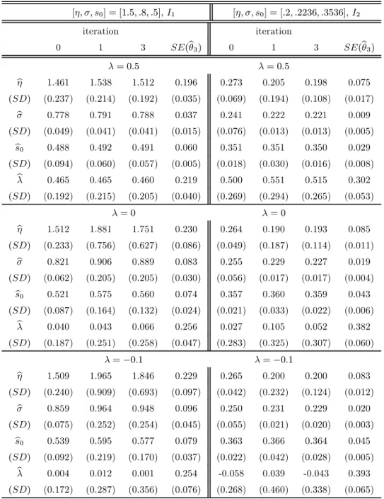
In ourfinal set of experiments we turn from the baseline intexpOU process to the more general
Box Cox transformed model. The econometrician observes the intinvBCOU process S(kλ). We
reconsider the previous settings, and consider three cases for the Box Cox parameterλ, namely
λ= 0.5,λ= 0, andλ=−0.1.
Table 4 reports the results. Forλ= 0.5, all the estimates are very good across the investigated
settings. The SDs diminish across the iterations, and the average SEs are in good agreement with
[η, σ, s0] = [1.5, .8, .5],I1 [η, σ, s0] = [.2, .2236, .3536],I2 iteration iteration 0 1 3 SE(eθ3) 0 1 3 SE(eθ3) λ= 0.5 λ= 0.5 e η 1.461 1.538 1.512 0.196 0.273 0.205 0.198 0.075 (SD) (0.237) (0.214) (0.192) (0.035) (0.069) (0.194) (0.108) (0.017) e σ 0.778 0.791 0.788 0.037 0.241 0.222 0.221 0.009 (SD) (0.049) (0.041) (0.041) (0.015) (0.076) (0.013) (0.013) (0.005) e s0 0.488 0.492 0.491 0.060 0.351 0.351 0.350 0.029 (SD) (0.094) (0.060) (0.057) (0.005) (0.018) (0.030) (0.016) (0.008) e λ 0.465 0.465 0.460 0.219 0.500 0.551 0.515 0.302 (SD) (0.192) (0.215) (0.205) (0.040) (0.269) (0.294) (0.265) (0.053) λ= 0 λ= 0 e η 1.512 1.881 1.751 0.230 0.264 0.190 0.193 0.085 (SD) (0.233) (0.756) (0.627) (0.086) (0.049) (0.187) (0.114) (0.011) e σ 0.821 0.906 0.889 0.083 0.255 0.229 0.227 0.019 (SD) (0.062) (0.205) (0.205) (0.030) (0.056) (0.017) (0.017) (0.004) e s0 0.521 0.575 0.560 0.074 0.357 0.360 0.359 0.043 (SD) (0.087) (0.164) (0.132) (0.024) (0.021) (0.033) (0.022) (0.006) e λ 0.040 0.043 0.066 0.256 0.027 0.105 0.052 0.382 (SD) (0.187) (0.251) (0.258) (0.047) (0.283) (0.325) (0.307) (0.060) λ=−0.1 λ=−0.1 e η 1.509 1.965 1.846 0.229 0.265 0.200 0.200 0.083 (SD) (0.240) (0.909) (0.693) (0.097) (0.042) (0.232) (0.124) (0.012) e σ 0.859 0.964 0.948 0.096 0.250 0.231 0.229 0.020 (SD) (0.075) (0.252) (0.254) (0.045) (0.055) (0.021) (0.020) (0.003) e s0 0.539 0.595 0.577 0.079 0.363 0.366 0.364 0.045 (SD) (0.092) (0.219) (0.170) (0.037) (0.022) (0.042) (0.028) (0.005) e λ 0.004 0.012 0.001 0.254 -0.058 0.039 -0.043 0.393 (SD) (0.172) (0.287) (0.356) (0.076) (0.268) (0.460) (0.338) (0.065)
Table 4: Simulation evidence: Estimating the parameters of the Box Cox transformed model.
explains the occasional discrepancy between SDs and average SEs for iteration 3. Relatedly, the
unweighted estimator is preferred to the weighted estimator in thefirst setting and forλ=−0.1
the mean estimate fails to pick up the sign ofλas the mean estimate is statistically insignificant,
but recall that time aggregation in this setting is substantial. By contrast, the mean estimate ofλ
correctly picks up the sign in the second setting. The results forλ= 0should also be compared
to the results for the intexpOU process of Table 2. It is clear that the combination of an
unconstrained estimation ofλand the use of fourth order approximations leads to no significant
deterioration of the estimates. In summary, for sample sizes of 500, efficiency gains from iterated
estimation only arise forλ= 0.5, the unweighted estimator yields typically good results, and the
nested intexpOU population case is well estimated by the unconstrained estimator.
7
Empirical Application: Income Dynamics in the US.
We estimate the parameters of the structural continuous-time model using individual annual earnings data from the Panel Study of Income Dynamics (PSID).
7.1
The Data
The PSID data are provided in a standardized and easily accessible form by the Cross National
Equivalent Files (CNEF) project (Frick et al., 2007).9 We use a balanced panel of annual
observations from 1989 until 1996, a total of 8 waves. Sk,i are individual’s i labor earnings
in year k. These labor earnings include wages and salary from all employment including
self-employment as well as bonuses, overtime and commissions. Annual earnings are measured in current 10,000 US dollars.
Turning to sample selection, we consider full-time employees having worked at least 1,500
hours per year. We follow standard practice and remove extreme outliers that could influence
the estimation results by deleting the top and bottom 0.5% percent of observations in each
wave. Our Mincerian covariates include sex, age, age2, and years of education interpreted a
(pre-determined) measure of human capital. In order to capture the effect of economic growth,
we also include a time trend. Cohort effects are not identified when age and time are regressors
present (Deaton and Paxson, 1994).
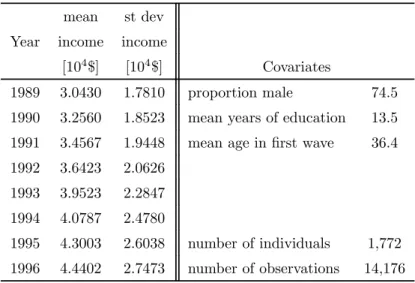
Table 5 reports some cross-sectional summary statistics of income. The number of persons
in the panel isN = 1,772.The average age in thefirst wave is 36.4. Since the panel is balanced,
average age increases by 1 each year.
mean st dev
Year income income
[104$] [104$] Covariates
1989 3.0430 1.7810 proportion male 74.5
1990 3.2560 1.8523 mean years of education 13.5
1991 3.4567 1.9448 mean age infirst wave 36.4
1992 3.6423 2.0626
1993 3.9523 2.2847
1994 4.0787 2.4780
1995 4.3003 2.6038 number of individuals 1,772
1996 4.4402 2.7473 number of observations 14,176
Table 5: PSID descriptive statistics.
Estimating a standard discrete-time random effects panel regression of log-earnings on
co-variates yields the following coefficient estimates (standard errors): sex: −0.319(0.022), years
of schooling: 0.114 (0.005), age: 0.081 (0.005), age squared: −0.00085(5.3×10⁻⁵) and linear
time trend: 0.038 (0.002). The variance of the individual effect is estimated as 0.153 while the variance of the idiosyncratic error term is 0.078. The principal interest, however, is the stochastic
structure of the continuous-time process{u(t)}.
7.2
Estimation Details
We estimate the model parameters by iterated GMM using the estimating equations described
in Section 5. The length of vectorf, i.e. the number of moment conditions used to identify the
parameters, is K(P + 1) = 8·6 = 48.10 We impose the stationarity restriction a= 0, i.e. the
variances2
0 of the initial deviationu(t0) is not estimated but calculated from the estimates of
η and σ2 using (6). This is a mild restriction since the impact of the initial deviation vanishes
over time if the OU process is stable.
7.3
Empirical Results
The estimates of the structural parameters are reported in Table 6. All parameters are
sta-tistically significant. The parameter estimates of β and γ are very plausible, close to the ones
1 0While there are six covariates (sex, education, age, age2, time trend, and a constant for the intercept) present,
we have to drop either the time trend or age from the list of covariates if we make the simplifying assumption in
parameter estimate SE BC model SE intercept μ −2.3296 0.2315 −1.4072 0.2407 sex β1 −0.3038 0.0583 −0.2281 0.0535 education β2 0.1254 0.0216 0.1084 0.0153 age γ1 0.0928 0.0063 0.0654 0.0063 age2 γ 2 −0.0010 0.0001 −0.0009 0.0001 time effect γ3 0.0407 0.0032 0.0360 0.0041 individual effect σ2 ε 0.1177 0.0125 0.0870 0.0225 OU parameter η 2.3240 0.6475 1.955 0.4835 diffusion coefficient σ2 0.5033 0.1990 0.3287 0.1286
Box Cox parameter λ - - −0.1098 0.0576
Table 6: Coefficient estimates of the intexpOU earnings process estimated using PSID data.
estimated in a naive panel regression (though the standard errors are considerably larger since the naive panel model neglects the intertemporal dependence), and are of the same magnitudes as reported in the literature. This should not be surprising given the result stated in Lemma 6. The implied estimated variance of the initial deviation equals the unconditional variance
ˆ s2
0= ˆσ2/(2ˆη) = 0.1083. As regards the interpretation of the parameters of the OU process, this
is perhaps best done visually in terms of their implications on moments and the cross-sectional
income distribution. Figure 1 (a) and (b) displays the goodness offit of the model by comparing
empirical sample moments of income and the moments predicted by the estimated model. It is evident that the moments are well estimated.
The estimates of the parameters of the Ornstein-Uhlenbeck component,ˆηandσˆ2, imply that,
given the individual effect εi, deviations from the expected log-income path decline relatively
rapidly: The percentage deviation of the latent continuous-time income Yit from its mean is
expected to halve in about four months. In order to gauge the relative influence of the individual
effect on the distribution we compute the cross-sectional coefficient of variation of the continuous-time process, CV(Yit) = p V ar(Yit) E(Yit) = sµ exp µ σ2 ε+ σ2 2η ¶ −1 ¶ .
Inserting our parameter estimates yieldsCVd= 0.5035.Settingσ2
ε= 0to eliminate the individual
effects the coefficient of variation decreases to0.3382, while settingσ2= 0to eliminate the error
process results in CVd = 0.3534. Even though the two components are not additive we can
conclude that the influence of the individual effect and the error process on the distribution is of
1989 1991 1993 1995 2. 5 3 .0 3. 5 4 .0 4. 5 5 .0
(a) First Moments
Year M e a n I n c o m e ( 10. 000 $) 1989 1991 1993 1995 2. 5 3 .0 3. 5 4 .0 (b) Autocovariances Year A u to co va ri a n c e 0 2 4 6 8 10 12 14 0. 0 0 0. 10 0. 20 0. 3 0 (c) Distribution 1989 Income (in 10.000 $) 0.5 1.0 1.5 2.0 2.5 3.0 -1 0 -8 -6 -4 -2 0 (d) Pareto plot log(x) lo g( 1-F (x ))
Figure 1: (a) Empirical means (solid line) and model impliedfirst moments (dashed line); (b)
empirical (solid) and theoretical (dashed) variances in 1989 and autocovariances between 1989 and 1990, . . . , 1996; (c) histogram and model implied density of income 1989; (d) empirical (solid) and theoretical (dashed) Pareto plots of income 1989
We proceed to consider the entire income distribution. Lemma 2 states that the income density implied by the structural model is not tractable analytically. We therefore estimate the
income density by Monte Carlo methods. In particular, we simulate income paths ofB= 20,000
individuals having the same distribution of covariates as the original data. Figure 1 (c) depicts the histogram of the actual incomes for the year 1989, and the kernel density estimate of the simulated incomes. The model-based simulated density describes the actual income density well. Finally, Figure 1 (d) shows the Pareto plots of the 1989 income data and the corresponding
Pareto plot of the simulated incomes. Recall that a Pareto plot depicts log (1−F(x)) versus
log (x). If the distribution is heavy-tailed, i.e. 1−F(x) = x−1/γL0(x) for sufficiently large
xwhere L0 is a slowly varying function and γ >0, then the plot is a straight line with slope
−1/γ for sufficiently largex. As regards the theoretical Pareto plot, we know from Lemma 4
that the intexpOU process cannot generate heavy tails. This manifests itself in the curvature of the theoretical Pareto plot in the extreme right tail. However, Figure 1 (d) reveals that the empirical Pareto plot becomes a straight line in the rightmost tail of the income distribution. In
particular, by inspection, the plot suggests the estimate1/bγ≈ −11.
In the light of this tails behavior, we estimate the generalized model for the intinvBCOU process, in which the estimated Box Cox parameter, if negative, picks up the heavy tail. Table 6 reports the results. The Box Cox parameter is indeed estimated to be negative, but is small in
magnitude and only marginally significant. Lemma 7 and the Remark following its proof in the
Appendix state thatγ =|λ|−1 when λ <0. The point estimatebλ=−.1suggests an estimate
of γ which is very close to the slope of the Pareto plot in its right tail obtained by inspection.
Turning to the the remaining covariate coefficients reported in the Table, these hardly change,
while the estimates of the interceptμand the OU drift parameterηhave fallen in magnitude.
We summarize all this evidence by concluding that the estimated structural model of the intexpOU describes the empirical US earnings distributions and the intertemporal dependencies very well. Like all standard earnings models in the literature, the process generates a right tail of the earnings distribution which decays too fast, but this tail behavior is captured by the computationally more intensive generalized model of the intinvBCOU process. However, the difference in tail decay between the two models is not “too large”, so that for most applications the simpler intexpOU process provides a good description of all the features of the US earnings distribution.
8
Conclusion
We have considered continuous-time earnings models and their associated observable, time ag-gregated or ‘integrated’, processes. We have shown that time aggregation alters important sta-tistical properties, for instance the integrated process does not inherit the lognormality and Markovianess of the underlying continuous-time process. The parameters of this process are
estimable by GMM, and the finite sample performance of the estimator is shown to be good
in several simulation studies. When applied to US panel data, the estimated models replicate well all important features of the actual earnings distribution. While the computationally more demanding intinvBCOU process does capture the heavy-tailedness of the actual earnings distri-bution, the estimate of the Box Cox parameter also reveals that the discrepancies between the speed of tail decays is relatively small. Hence we conclude that the simpler intexpOU process does a good job in describing the actual US earnings distributions.
References
Abowd, J. and D. Card(1989), “On the covariance structure of earnings and hours changes”,
Econometrica, 57, 411-445.
Baker, M. (1997), “Growth-rate heterogeneity and the covariance structure of life-cycle
earn-ings”,Journal of Labor Economics, 15, 338-375.
Barndorff-Nielsen, O. E. and N. Shepard (2001), “Non-Gaussian
Ornstein-Uhlenbeck-based models and some of their uses infinancial econometrics (with discussion)”,J. Roy. Statist.
Soc. Ser. B,63, 167-241.
Bhattacharya, R., E. Thomann, and E. Waymire (2001), “A note on the distribution of
integrals of geometric Brownian motion”,Statistics and Probability Letters,55, 187-192.
Bick, B., H. Kraft and C. Munk(2009), “Investment, income, and incompleteness”, working
paper.
Bodie, Z., Merton, R.C. and W.F. Samuelson(1992), “Labor supplyflexibility and
port-folio choice in a life-cycle model”,Journal of Economic Dynamic and Control, 16(3-4), 427-449.
Carr, P. and M. Schröder (2004), “Bessel processes, the integral of geometric Brownian
motion, and Asian options”,Theory of Probability and Its Applications, 48, 400-425.
Christiano, L. J., M. Eichenbaum, and D. Marshall (1991), “The permanent income
Comte, F., V. Genon-Catalot, and Y. Rozenholc(2009), “Nonparametric adaptive
esti-mation for integrated diffusions”,Stochastic Processes and their Applications, 119, 811-834.
Deaton, A. and C. Paxson(1994), “Intertemporal choice and inequality”,Journal of Political
Economy, 102, 437-467.
Ditlevsen, S. and M. Sørensen (2004), “Inference for observations of integrated diffucion
processes”,Scandinavian Journal of Statistics, 31, 417-429.
Frick, J.R., S.P. Jenkins, D.R. Lillard, O. Lipps and M. Wooden(2007), “The
Cross-National Equivalent File (CNEF) and its Member Country Household Panel Studies”,Schmollers
Jahrbuch,127, 627-654.
Gloter, A. (2001), “Parameter estimation for a discrete sampling of an integrated
Ornstein-Uhlenbeck process”,Statistics, 35, 225-243.
Gloter, A.(2006), “Parameter estimation for a discretely observed integrated diffusion process”,
Scandinavian Journal of Statistics, 33, 83-104.
Guvenen, F. (2009), “An empirical investigation of labor income processes”, Review of
Eco-nomic Dynamics, 12, 58-79.
Harvey, A. C. and J. H. Stock(1989), “Estimating integrated higher-order continuous time
autoregressions with an application to money-income causality”, Journal of Econometrics, 42,
319-336.
Henderson, V.(2005), “Explicit solutions to an optimal portfolio choice problem with
stochas-tic income”,Journal of Economic Dynamics and Control, 29, 1237-1266.
Kaufmann, E.(2000), “Penultimate Approximations in Extreme Value Theory”,Extremes, 3,
39-55.
Koo, H.K.(1998), “Consumption and portfolio selection with labor income: a continuous time
approach”,Mathematical Finance, 8, 49-65.
MaCurdy, T.(1982), “The use of time series processes to model the error structure of earnings
in longitudinal data analysis”,Journal of Econometrics, 18, 83-114.
Munk, C. and C. Sørensen (2009), “Dynamic asset allocation with stochastic income and
interest rates”, working paper.
Newey, W.K. and D. McFadden(1994), “Large sample estimation and hypothesis testing”,
in: Handbook of Econometrics, chapter 36.
Pareto, V. (1896), “La courbe de la répartition de la richesse”, reprinted 1965 in G. Busoni
richesse, Geneva: Librairie Droz. English translation inRivista di Politica Economica, 87 (1997), 647-700.
Schluter, C. and M. Trede(2002), “Tails of Lorenz curves”,Journal of Econometrics, 109,
151-166.
Schluter, C. and M. Trede(2008), “Identifying multiple outliers in heavy-tailed distributions
with an application to market crashes”,Journal of Empirical Finance, 15, 700-713.
Wang, N., (2004), “Precautionary saving with partially observed income”,Journal of Monetary
Economics, 51, 1645-1681.
Wang, N.(2006), “Generalizing the permanent-income hypothesis: revisiting Friedman’s
con-jecture on consumption”,Journal of Monetary Economics, 53, 737-752.
Wang, N.(2009), “Optimal consumption and asset allocation with unknown income growth”,
A
Moment Expressions for the intexpOU Process with
˜
y
(
t
)
≡
0
The presence of covariates in they˜(t)process precludes us from saying much analytically, but in
the absence of they˜(t)process we can obtain some useful insights about the moments ofSk. For
expositional brevity we focus on regular intervals of length∆. For the first moment we obtain
an exact result. Exact results are also available in the stationary case (whena= 0), otherwise
we state approximations for variances and covariances.
Lemma 8 Consider the case when y˜(t)≡0and regular intervals of length∆. Then E(Sk)×exp µ −σ 2 4η ¶ =∆+ 1 2η ∞ X i=1 1 i 1 i! ha 2e −2η(tk−1)∆i i£ 1−e−2iη∆¤.
In the stationary case with a = 0, or asymptotically with k → ∞, we have E(Sk) =
∆exp¡σ2/4η¢, while the expectation becomes unbounded for∆→ ∞.
Exact expressions for covariances and variances are only available in the stationary case
considered explicitly below in Lemma 10. Asymptotics for k→ ∞ i.e. tk−1 → ∞ yield simple
results and are stated next, while approximations for the general case are stated below in Lemma 12.
A.1
Moments’ Asymptotics
Lemma 9 Consider the case when y˜(t)≡ 0, let η > 0 and consider regular intervals of fixed
length∆. Ask→ ∞ E{Sk} → exp µ σ2 4η ¶ ∆, Cov{Sl, Sk}lfixed → 0, V ar{Sk} ×exp µ −σ 2 2η ¶ 1 2 → 1 η ∞ X i=1 1 i 1 i! ∙ σ2 2η ¸iµ ∆+ 1 iη £ e−iη∆−1¤ ¶ .
A.2
The Exact Moments of
{
S
k}
in the Stationary Case
In the stationary casea= 0, and we can state exact expressions for the covariance structure:
length∆. Then E{Sk} = exp µ σ2 4η ¶ ∆ Cov{Sl, Sk}l<k×exp µ −σ 2 2η ¶ = 1 η ∞ X i=1 1 i 1 i! ∙ σ2 2η ¸i 1 iηe −iη∆(k−l) × £ eiη∆−1¤ £1−e−iη∆¤ V ar{Sk} ×exp µ −σ 2 2η ¶ 1 2 = 1 η ∞ X i=1 1 i 1 i! ∙ σ2 2η ¸iµ ∆+ 1 iη £ e−iη∆−1¤ ¶ .
Of course Lemma 10 specializes to Lemma 9 ask→ ∞.
Moreover, we can derive the spectral density for the stationary process.
Lemma 11 Consider the case wheny˜(t)≡0, let a= 0 and consider regular intervals of fixed
length∆. The spectral density is
fS(λ) = ∞ X j=1 cj 2π ∙ 1−e−2jη∆ 1−2e−jη∆cosλ+e−2jη∆ ¸ (16) withcj= exp ³ σ2 2η ´ 1 j 1 j! h σ2 2η ij 1 jη2 £ ejη∆+e−jη∆−2¤ andλ∈[−π, π].
The first order term in the series offS(λ), 2c1π
£
1−2e−η∆cosλ+e−2η∆¤−1, is the spectral
density of an AR(1) process with coefficient e−η∆, with the variance of the white noise error
equal toc1 and depending on the autoregressive coefficient.11
A.3
Covariance Approximations for the General Case
The exact expression for thefirst moment is stated above in Lemma 8. Exact expressions for
the covariance structure are not available in the general case, but we can state the following approximations:
Lemma 12 Consider the case wheny˜(t)≡0and assume that η >0. Then Cov(Sl, Sk)l<k×exp µ −σ 2 2η ¶ ' 1η ∞ X i=1 1 i 1 i! ∙ σ2 2η ¸i 1 iη £
eiη∆−1¤ £1−e−iη∆¤e−iη(k−l)∆− 1 2η ∞ X i=1 1 i 1 i! ha 2 ii 1 2iηe −2iη(l−1)∆£e−2iη∆ −1¤2e−2iη(k−1)∆.
1 1For completeness we also state the spectral density of the underlying continuous process as f
Y(λ) = 1 2πσ 2expqσ2 2η r S∞ j=1j1! σ2 2η j 2jη 1 j2η2+λ2 forλ∈R.
V ar{Sk} ×exp µ −σ 2 2η ¶ ' 2 η ∞ X i=1 1 i 1 i! ∙ σ2 2η ¸iµ ∆+ 1 iη £ e−iη∆−1¤ ¶ − 1 2η ∞ X i=1 1 i 1 i! ha 2 ii 1 2iη £ e−2iη∆−1¤2e−4iη(k−1)∆. The order of the approximation is a∆1ηe−η(k−1)∆£1−e−η∆¤.
In the stationary case a= 0 and this covariance and variance immediately simplify to the
statement in Lemma 10, while withtl−1fixed andtk−1→ ∞we immediately obtain the statement
of Lemma 9. Similar approximations can be derived for the caseη <0.
B
Proofs
We briefly state two Lemmas which will be used in the subsequent proofs.
Lemma 13 Let X = (X1, . . . , XT)> be a multivariate normal random variable. Its moment
generating function is MX(θ)≡E ³ eθ>X´= exp µ μ>θ+1 2θ >Σθ¶
whereμis the expectation vector and Σ= [σst] is the covariance matrix. The expectation of the
exponentiated sum is then
E¡eX1+...+XK¢=M X(1) = exp ÃK X k=1 μk+1 2 K X k=1 K X r=1 σkr ! , (17)
andY = exp(X)is multivariate lognormal with expectations and covariances given by E(Yk) = exp µ μk+1 2σkk ¶ Cov(Yk, Yr) = exp µ (μk+μr) +1 2(σkk+σrr) ¶ (exp (σkr)−1).
Direct computations lead to the following lemma.
Lemma 14 The process{y˜(t) :t≥t0}is Gaussian with
E(˜y(t)) = μ+Z1>β+Z2>,tγ Cov(˜y(s),y˜(t)) = σ2ε,
and the process{u(t) :t≥t0}is Gaussian with E(u(t)) = 0 Cov(u(s), u(t)) = ∙ s20+σ 2 2η ³ e2ηmin(s,t)−1´¸e−η(t+s) = ∙ σ2 2ηe −η(t−s)+e−η(t+s) µ s2 0− σ2 2η ¶¸ s≤t .
Proof of Proposition1. By direct computation using the Lemmas 13 and 14. In particular
{Y (t) :t≥t0}is a log-normal process. Finally, {exp (u(t))} is Markov since u(t) is, because
the increments are independent, and {Y (t)}is Markov given the independence of {y˜(t)} and
{u(t)}.
Proof of Lemma2. The distribution ofSkhas no closed form expression, since the distribution
of the sum of dependent log-normal variates has no exact closed form. As regards the non-Markov
property, only consider the OU process and intervals of equal length 0 =t0 < t1 = ∆< t2 =
2∆< . . . < tT =T∆. Using (4) wefind Sk = Z k∆ (k−1)∆ exp (u(t))dt = Z ∆ 0 exp à u((k−1)∆)e−μt+σ Z (k−1)∆+t (k−1)∆ eμ(s−t)dWs ! dt.
If the value of the latent process at the beginning of the interval,u((k−1)∆), was known,Sk
would not depend onSk−1, Sk−2, . . .However, since the process u(t) is latent we can only use
the conditional distribution ofu((k−1)∆)given Sk−1, Sk−2, . . . to determine the distribution
ofSk. As the same holds true forSk−1 andu((k−2)∆), the process{Sk:k= 1, . . . , T}cannot
be Markov.
Proof of Lemma7. We recall some results from extreme value theory (EVT). The Generalized Extreme Value distribution is given by
G(x) = exp³−h1 +γ
σ(x−μ)
−1/γ
+
i´
whereγis the shape parameter of interest. It is the limit distribution of the normalized maximum
of a random variable X with distribution FX (if the limit exists). γ > 0 is the Frechet case,
so FX is heavy tailed, γ →0is the Gumbel case so FX is slowly varying in its right tail, and
γ <0is the negative Weibull case. Let xF be the upper end point of the distributionFX, and
lethX(x) = 1−fXFX(x()x) be the reciprocal of the hazard function. A well-known result from EVT
(Kaufmann, 2000) states thatγX = limx→xFh0X(x).
Consider the Box Cox transformation g(x) = xλλ−1 with x > 0 and λ 6= 0. For later
reference we haveg0(x) =xλ−1andg00(x) = (λ−1)xλ−2sog00(x)/[g0(x)]2
= (λ−1)x−λ. Let
Y =g−1(U). We prove the result stated in the Lemma more generally for distributions ofU
which lie in specific domains of attractions which depend on the sign of λ.
We have
The associated density isfY(y) =fU(g(y))g0(y),and hY (y) = 1−FY (y) fY (y) = 1−FU(g(y)) fU(g(y)) 1 g0(y) = hU(g(y)) 1 g0(y).
Differentiating the latter yields
h0Y(y) =h0U(g(y))−hU(g(y))
g00(y) [g0(y)]2.
In the particular case of the Box Cox transform,g00(y)/[g0(y)]2= (λ−1)y−λ, so
γY =γU−(λ−1) lim
y→yF
hU(g(y))y−λ. (19)
As regards the Box Cox parameterλ, we distinguish between three cases.
Case (a) If λ > 0, assume that the distribution of U is in the domain of attraction of the
Gumbel distribution, so that
hU(x) =Cx−α
¡
1 +O¡x−ε¢¢
withα >−1, ε >0andC >0. This class includes the normal distribution withα= 1and the
lognormal distribution withα= 0. We haveyF =∞. Thenh0u(x) =−αCx−(α+1)(1 +O(x−ε)),
and thusγU = limx→∞h0u(x) = 0. Moreover
hU(g(y))y−λ=Cλ−α
£
yλ−1¤−αy−λ³1 +O³£yλ−1¤−ε´´.
Then limy→∞hU(g(y))y−λ = 0 for α ≥0. We have the result that γY = 0 so FY is slowly
varying in its right tail.
Case (b) When λ = 0, h0Y (y) = h0U(g(y)) + limy→∞hU(g(y)), with g(y) = ln (y) so for
α≥0,γY = 0again.
Case (c) Next, consider λ <0. Theng has an asymptote at|λ|−1, so thatU cannot exceed
|λ|−1. Assume that the distribution ofU satisfies this restriction. In particular, the distribution
of U could be normal but truncated at uF → |λ|−1so that yF = g−1(uF). Therefore the
distribution of U is now in the domain of attraction of the (negative) Weibull distribution, so
that 1−FU(u) =C(uF−u)α h 1 +D(uF−u)β+O ³ (uF −u)β+ε ´i (20) withα, β, ε, C >0andD∈R, and uF <∞. Then
fU(u) =αC(uF−u)α−1 h 1 + ((α+β)/α)D(uF −u)β+O ³ (uF−u)β+ε ´i
and hU(u) =α−1(uF−u) 1 +D(uF−u)β+O ³ (uF−u)β+ε ´ 1 + ((α+β)/α)D(uF−u)β+O ³ (uF−u)β+ε ´.
It follows that γU = limu→uFh
0
U(u) = −α−1. The Box Cox transform is g(x) = 1−x
−|λ| |λ| and g00(y)/[g0(y)]2 =−(1 +|λ|)y|λ|, so γY =γU+ (1 +|λ|) lim y→yF hU(g(y))y|λ|.
We have foruF →|λ|−1 and thusyF → ∞
lim y→∞hU(g(y))y |λ| = lim y→∞α −1 µ |λ|−1−1−y −|λ| |λ| ¶ y|λ| = lim y→∞α −1 µ y−|λ| |λ| ¶ y|λ| = α−1|λ|−1. In summary γY = −α−1+ (1 +|λ|)α−1|λ|−1 = α−1|λ|−1.
ThereforeγY >0and the distribution is heavy-tailed.
Remark 15 If the distribution ofU is a truncated normal distribution, thenFU is in the domain
of attraction of the negative Weibull distribution given by (20) withα= 1, and thenγY =|λ|−
1 ifλ <0. Proof: Consider 1−FU(u) =c 1 √ 2πσ Z uF−u 0 exp à −1 2 µ (u−μ) +ε σ ¶2! dε.
The claim follows using a Taylor expansion aboutε= 0.
For the next set of proofs, the following result is useful.
Lemma 16 Define the error integral by EI(y;ea)≡ Z exp ( e ay) y dy= logy+ e ay 1 + 1 2 (eay)2 2! + 1 3 (eay)3 3! +.. (21)
Then Z tk tk−1 exp¡eaebt¢dt = µ1 b ¶ Z τk τk−1 exp (eay) y dy = µ 1 b ¶ EI(y;ea)|eebtkbtk−1 = tk−tk−1+ 1 b ∞ X i=1 1 i 1 i!ea i£eibtk −eibtk−1¤.
The Lemma follows after the change of variablesy=ebtwith inverse Jacobian∂y/∂t=by.
Proof of Lemma8. We have
E{Sk} = Z ∆ τ=0 E{Y (tk−1+τ)}dτ = exp µ σ2 4η ¶ Z ∆ τ=0 exp³a 2e −2ηtk−1e−2ητ´dτ . Hence using Lemma 16 we obtain
E{Sk} ×exp µ −σ 2 4η ¶ =∆− 1 2η ∞ X i=1 1 i 1 i! ha 2e −2ηtk−1i i£ e−2ηi∆−1¤. Proof of Lemma9.
(i) The expression for thefirst moment follows immediately from Lemma 8.
(ii) The covariances. Fixsand apply Proposition 1. Then
lim t→∞Cov(Y (s), Y (t))s<t×exp µ −σ 2 2η ¶ = 0 and therefore lim tk−1→∞ Cov{Sl, Sk}tl−1fixed = lim t→∞ Z tl−1+∆ s=tl−1 (Z ∆ τ=0 Cov(Y(s), Y (tk−1+τ))dτ ) ds = 0.
(iii) The variances. Letting boths, t→ ∞we have by Proposition 1
Cov(Y (s), Y (t))s<t×exp µ −σ 2 2η ¶ → exp µ σ2 2ηe −η(t−s) ¶ −1, Cov(Y (s), Y (t))s>t×exp µ −σ 2 2η ¶ → exp µ σ2 2ηe −η(s−t) ¶ −1.
Then V ar{Sk} = Z tk t=tk−1 Z t s=tk−1 Cov(Y(s), Y (t))dsdt + Z tk t=tk−1 Z tk s=t Cov(Y (s), Y (t))dsdt
By Lemma 16 withea=¡σ2/2η¢e−ηt we have
Z t s=tk−1 exp (eaeηs)ds = (t−tk−1) + 1 η ∞ X i=1 1 i 1 i!ea i¡eiηt −eiηtk−1¢ = (t−tk−1) + 1 η ∞ X i=1 1 i 1 i! ∙ σ2 2η ¸i ¡ 1−e−iηteiηtk−1¢
Therefore integrating overtyields
exp µ −σ 2 2η ¶ × Z tk t=tk−1 Z t s=tk−1 Cov(Y(s), Y (t))dsdt = ∆ η ∞ X i=1 1 i 1 i! ∙ σ2 2η ¸i + 1 η2 ∞ X i=1 1 i2 1 i! ∙ σ2 2η ¸i £ e−iη∆−1¤.
A similar calculation forexp¡−σ2/2η¢×Rtk
t=tk−1 Rtk−1
s=t Cov(Y (s), Y (t))dsdtyields the same
result, so putting everything together, we have
V ar{Sk}exp µ −σ 2 2η ¶ 1 2 → ∆ η ∞ X i=1 1 i 1 i! ∙ σ2 2η ¸i + 1 η2 ∞ X i=1 1 i2 1 i! ∙ σ2 2η ¸i £ e−iη∆−1¤.
Proof of Lemma10. Use similar calculations as in the proof of Lemma 9.
Proof of Lemma11. Using Lemma 10 withk=l+hthe autocovariance function is, for allh,
γS(h) =
∞
X
j=1
with b =η∆>0and cj = exp ³ σ2 2η ´ 1 j 1 j! h σ2 2η ij 1 jη2 £
ejη∆+e−jη∆−2¤. The spectral density is
defined asfS(λ) =21πPh∞=−∞e−iλhγS(h)fori=
√
−1. Considerfirst thefirst order term
e fS(λ) = 1 2π ∞ X h=−∞ e−iλhc1e−b|h| = c1 2π ⎡ ⎣1 + ∞ X h≥1 ³ e−(iλ+b)´ h + −∞ X h≤−1 ³ e−(iλ−b)´ h ⎤ ⎦ = c1 2π ⎡ ⎣1 + ∞ X h≥1 ³ e−(iλ+b)´h+ ∞ X h≥1 ³ e(iλ−b)´h ⎤ ⎦ = c1 2π ∙ 1 + e− (iλ+b) 1−e−(iλ+b) + e(iλ−b) 1−e(iλ−b) ¸ = c1 2π ∙ 1−e−2b 1−e−b(eiλ+e−iλ) +e−2b ¸ = c1 2π ∙ 1−e−2b 1−2e−bcosλ+e−2b ¸ .
The spectral density is therefore
fS(λ) = ∞ X j=1 cj 2π ∙ 1−e−2jb 1−2e−jbcosλ+e−2jb ¸ .
Remark: The spectral density of the underlying continuous-time processY (t)is
fY (λ) = 1 2πσ 2exp ½ σ2 2η ¾X∞ j=1 µ σ2 2η ¶j 2jη 1 j2η2+λ2.
Proof. The autocovariance function is
γY (h) = exp ½ σ2 2η ¾∙ exp ½ σ2 2ηe −η|h| ¾ −1 ¸ .