Boston University
OpenBU http://open.bu.edu
Mathematics and Statistics BU Open Access Articles
2018
How the instability of ranks under
long memory affects large-sample
inference
This work was made openly accessible by BU Faculty. Please share how this access benefits you. Your story matters.
Version Accepted manuscript
Citation (published version): Shuyang Bai, Murad S Taqqu. 2018. "How the instability of ranks under long memory affects large-sample inference." Statistical Science, Volume 33, Issue 1, pp. 96 - 116.
https://doi.org/10.1214/17-STS633 https://hdl.handle.net/2144/39120
arXiv:1610.00690v2 [math.ST] 2 Nov 2017
Submitted to Statistical Science
How the instability of ranks under
long memory affects large-sample
inference
Shuyang Bai , Murad S. Taqqu∗
University of Georgia and Boston University
Abstract. Under long memory, the limit theorems for normalized sums of random variables typically involve a positive integer called “Hermite rank”. There is a different limit for each Hermite rank. From a statis-tical point of view, however, we argue that a rank other than one is unstable, whereas, a rank equal to one is stable. We provide empirical evidence supporting this argument. This has important consequences. Assuming a higher-order rank when it is not really there usually re-sults in underestimating the order of the fluctuations of the statistic of interest. We illustrate this through various examples involving the sample variance, the empirical processes and the Whittle estimator.
Key words and phrases: Long-range dependence, Long memory, Her-mite rank, power rank, non-Gaussian limit, instability, large-sample inference.
1. INTRODUCTION
Suppose that D is a data set, and one has a statistical model for D which involves a random
stationary sequence {X(n)}, referred to as noise. Let T =T(D) be a sample statistic of interest.
Deriving the asymptotic distribution for the statistic T as the sample size tends to infinity is a
standard practice in large sample inference. The asymptotic distribution is useful for reporting confidence intervals, conducting hypothesis tests, etc.
When the construction of the statistic T involves summing the data and if the stationary noise
{X(n)} is weakly dependent, then the asymptotic distribution of T is typically Gaussian in view
of the Central Limit Theorem. This asymptotic distribution can also be a functional of a Gaussian process.
The situation, however, is much more intricate when the strength of dependence in the noise
increases significantly. This strong-dependence regime, often called long memory or long-range
Shuyang Bai: Department of Statistics, University of Georgia, Athens, GA 30602, US (e-mail: [email protected]). Murad S. Taqqu: Department of Mathematics and Statistics, Boston University, Boston, MA 02215, US (e-mail: [email protected]).
∗Supported by NSF grant DMS-1309009 at Boston University
2010 AMS Classification:62M10, 60F05
1
dependence, is typically characterized by the following behavior of the variance of partial sums: (1) Varh N X n=1 X(n)i≈N2H, asN → ∞.
where ≈means asymptotic equivalence up to some positive constant, the parameter H ∈(1/2,1)
is called the Hurst index1. Normally when the dependence is weak, one expects H = 1/2 in (1),
that is, the growth of the variance is linear. The superlinear growth in (1) is typically due to the
slow decay of the covariance of {X(n)}:
(2) Cov[X(n), X(0)]≈n2H−2, asn→ ∞,
where −1 <2H−2<0. In fact, (2) is also a common characterization of long memory. We refer the reader to the recent monographs Beran et al. [11], Giraitis et al. [39], Samorodnitsky [69] and
Pipiras and Taqqu [64] for comprehensive introductions to the notion long memory.
In view of (1), when deriving the asymptotic distribution of the sum, one needs to associate the
stronger normalization N−H to PN
n=1X(n) rather than the standardN−1/2 normalization. These
limit theorems have been applied in many statistical studies. See Section 3 below.
This paper makes the following basic argument: while these limit theorems are definitely of probabilistic interest, their immediate application to statistical inference can lead to problems. This is because these limit theorems can be unstable, that is, they often cease to hold when{X(n)} is slightly perturbed. In particular, the limit theorems under long memory often depend critically
on an integer quantity called rank, e.g, the Hermite rank in the Gaussian context. We will show
that the rank is unstable when it takes value greater than one, and it easily collapses to rank one when there is a slight perturbation.
The notion of rank, however, is not relevant when the data is weakly dependent. We indicate that under weak dependence, limit theorems are robust against, for example, a transformation of the data. We illustrate this by considering various types of weak dependence, such as strong mixing, Gaussian subordination and Bernoulli shifts.
The paper is organized as follows. The rank instability issue is discussed in Section2. In Section
3, we provide some examples on how the instability of rank can affect statistical results. In Section
4, we carry out an empirical study which supports the instability argument. In contrast, we show in
Section5that the central limit theorems under weak dependence are not subject to such instability
issues. Section 6 contains conclusions and suggestions. Some technical extensions are found in the
Appendix.
2. THE INSTABILITY OF RANKS UNDER LONG MEMORY
In this section, we introduce the notion Hermite rank and point out its instability. We focus on the simple scenario of instantaneous transformation of a Gaussian stationary process. (The
non-instantaneous case is somewhat technical and is deferred to AppendixA.) We then address the case
where the model involves a non-Gaussian linear (moving-average) process, where the corresponding
notion of Hermite rank is called the Appell rank or thepower rank.
Throughout the paper, the notation a(n) ≈b(n) means limn→∞a(n)/b(n) =cfor some generic
constant 0< c <∞ that can change from expression to expression. We note that in many places,
1
The term “Hurst index” is also frequently used for the self-similarity parameter of self-similar processes arising from the normalized limit of the sum of X(n) (see Pipiras and Taqqu [64]). It is also common to introduce the so-called memory parameterdin the context of (2), re-expressed as Cov[X(n), X(0)]≈n2d−1 (d=H−1/2). We will
useH throughout in order not to switch between parameters and thus to avoid confusion.
one can include a slowly varying function in the asymptotic relation, for example, a logarithmic function (see, e.g., Bingham et al. [14]), but for simplicity we do not do that.
2.1 Transformation of Gaussian processes
We want to consider possibly nonlinear finite-variance transformations of Gaussian random
vari-ables. To do so, let Z be a standard normal random variable, γ(dx) be the standard Gaussian
measure (2π)−1/2e−x2
/2dxon R, and let
L2(γ) ={G(·) : EG(Z)2 <∞}.
It is well-known (see, e.g., see Pipiras and Taqqu [64], Proposition 5.1.3) that{√1
m!Hm(·), m≥0}
forms an orthonormal basis of L2(γ), where {Hm(·), m≥ 0} are Hermite polynomials defined as
H0(x) = 1 and (3) Hm(x) = (−1)mex 2 /2 d dxme− x2 /2 for m ≥1.
Thus H1(x) =x,H2(x) = x2−1 and H3(x) =x3−3x, etc. We can now define the Hermite rank
of a functionG∈L2(γ).
Definition 2.1. Suppose thatG(·) ∈L2(γ). LetZ be a standard Gaussian random variable. The Hermite rank kof G(·) is defined as
(4) k= inf m≥1 : EG(Z)Hm(Z) = Z R G(x)Hm(x)γ(dx)6= 0 .
whereHm(·) is them-th order Hermite polynomial.
Remark 2.2. An alternative way of defining the Hermite rankkis through the starting index of the Hermite expansion of G(·)−EG(Z), namely,
(5) G(·)−EG(Z) =
∞
X m=k
cmHm(·), k≥1,
for some sequence cm satisfying ck 6= 0, where the series converges in the L2(γ)-sense. By the
orthonormality of{√1
m!Hm(·)}, we have
(6) cm= E
[G(Z)Hm(Z)]
m! for m≥0.
Note that c0 =EG(Z) sinceH0(Z) = 1. Furthermore, since the Hermite polynomials {Hm(·),0≤
m ≤ k} form a basis for polynomials of degree less than equal to k, the definition (4) can be
re-expressed as
(7) k= infnm≥1 : Eh G(Z)−EG(Z)Zmi6= 0o.
Remark 2.3. The Hermite rank ofG(x) is the same as that of G(x) +a, for any a∈R, since relation (5) involves centering.
Now suppose that{X(n)} is a long-memory stationary Gaussian process satisfying (2). We may assume without loss of generality that it is standardized, that is, EX(n) = 0 and Var[X(n)] = 1 The following lemma explains the role that the Hermite rank plays in determining the asymptotic behavior of the covariance of the transformed sequence{G(X(n))} (see p.223 of Beran et al. [11]).
Lemma 2.4. If G(·) has Hermite rank k, then
(8) Cov[G(X(n)), G(X(0))] ≈Cov[X(n), X(0)]k ≈n(2H−2)k.
Remark 2.5. Comparing (8) and (2), we note that for functionsG(·) that have Hermite rank
k = 1, the Hurst index of{G(X(n))} is the same as the Hurst index of {X(n)}. In general since
2H−2 < 0, the higher the Hermite rank k is, the faster the covariance decays as n→ ∞. Note
that in view of (2) and (8), for{G(X(n))} to have long memory, one needs (2H−2)k >−1 ⇐⇒ H >1− 1
2k.
This is natural because whenk >1, the covariance of{G(X(n))}decays faster than that of{X(n)} and thus H must be greater than 1−1/(2k) in order to ensure that {G(Xn)}has long memory.
2.2 Asymptotic behavior
Now returning to the theme of the introduction: suppose that in order to derive the asymptotic
distribution of the statistics T of interest, one first needs to obtain the distributional limit as
N → ∞ of (9) 1 A(N) [N t] X n=1 G(X(n))−EG(X(n)), t∈[0,1],
whereG(·)∈L2(γ), A(N) is a suitable normalization, and [·] stands for the integer part.
Theorem 2.6. (Dobrushin and Major [31], Taqqu [76], Breuer and Major [15], Major [57].)
Suppose that Ghas Hermite rank k. Then the following conclusions hold. • Central limit case: suppose that
H <1− 1 2k.
Then {G(X(n))} has short memory in the sense that
σ2 :=
∞
X n=−∞
Cov[G(X(n)), G(X(0))]
converges absolutely and
(10) 1 N1/2 [N t] X n=1 G(X(n))−EG(X(n))f.d.d.−→ σB(t), t≥0,
where f.d.d.−→ denotes convergence of the finite-dimensional distributions and B(t) is the standard Brownian motion.
• Non-central limit case: suppose that
H >1− 1 2k.
Then {G(X(n))} has long memory with Hurst index:
(11) HG= (H−1)k+ 1∈ 1 2,1 . Furthermore, as N → ∞, we have2 (12) 1 NHG [N t] X n=1 G(X(n))−EG(X(n))f.d.d.−→ cZHG,k(t),
for some c6= 0, and
(13) ZHG,k(t) = Z ′ Rk Z t 0 k Y j=1 (s−xj)γ+ds B(dx1). . . B(dxk), γ =H− 3 2 = HG−1 k − 1 2,
is the so-called k-th order Hermite process, where RR′k[ · ] B(dx1). . . B(dxk) denotes the k-tuple
Wiener-Itˆo integral with respect to the standard Brownian motion B(·). The prime ′ indicates that
one does not integrate on the diagonals xi=xj.
Remark 2.7. When the Hermite rank k= 1, one has
HG=H
and the limit ZHG,k(t) in Theorem 2.6 is the fractional Brownian motion BH(t), namely, the
centered Gaussian process determined by the following covariance structure: Cov [BH(s), BH(t)] =
1 2 |s|
2H+|t|2H − |s−t|2H.
The preceding covariance is shared by all the other Hermite processes. When the Hermite rank
k= 2,ZHG,2(t) is called theRosenblatt process (see Rosenblatt [68] and Taqqu [75]). The Hermite processZHG,k(t) in (13) admits different representations. See Pipiras and Taqqu [63].
Remark 2.8. The boundary case H = 1− 21k typically falls in the central limit theorem
regime (convergence to Brownian motion) after modifying the normalization N−1/2 to include
some slowly varying functions (Theorem 1’ of Breuer and Major [15]). In general, the convergence
of finite-dimensional distributionsf.d.d.−→ in the short-memory case cannot be strengthened to weak
convergence ⇒ in D[0,1] unless some additional assumption is imposed on G, e.g., G being a
polynomial (Chambers and Slud [17]).
The long-memory Gaussian{X(n)}may be directly used as a model for the long-memory
station-ary noise. For statistical theory, however, it is often desirable to allow departure from Gaussianity, e.g., to accommodate the situations where the noise distribution is skewed or heavy-tailed. Within the same framework, a way to achieve such flexibility is as follows. Suppose that there is an
un-derlying long-memoryGaussian stationary process{Y(n)}. Assume without loss of generality that
{Y(n)}is standardized. Now suppose that the noise sequence {X(n)}in the model is given by
(14) X(n) =F(Y(n)).
2
In fact, we have weak convergence in the spaceD[0,1] with uniform metric.
Remark 2.9. There are different perspectives to interpret (14). First, note that when F(·)
is nonlinear, X(n) is non-Gaussian. So F(·) can represent the departure from the ideal Gaussian
assumption. Hence when the noise X(n) is modeled by (14) with an unknown F(·), this provides
great model flexibility. Note that a proper choice of F(·) can match any marginal distribution for
X(n). Second, from the perspective of analysis of robustness, one may view X(n) as a perturbed
version ofY(n), whereX(n) is close to Y(n), that is, F(·) is close to the identity function.
Following the same statistical inference procedure that leads to (9), we then focus on the
distri-butional limit of 1 A(N) [N t] X n=1 G◦F(Y(n))−EG◦F(Y(n)) asN → ∞.
Remark 2.10. We emphasize the different roles played byF(·) and G(·). The function F(·)
accounts for an unknown and uncontrollable departure from the Gaussian Y(n). On the other hand, the function G(·) depends on the statistical procedure of interest and is therefore typically precisely known. For example,Gis typically the identity transformation for inference of the meanEX(n) =EF(Y(n)).
2.3 Basic claim
We are now ready to make the following claim which will be justified below. The case of
non-instantaneous (multivariate) F (and also G) will be addressed in Appendix A (the issues remain
essentially the same).
Claim 2.11. It is typically the case that
(a) the function G◦F has Hermite rank 1;
(b) the process {X(n)} has long memory with the same Hurst index H as {Y(n)} in (14).
Justification of the claim:. Let Z be standard Gaussian. SinceH1(Z) =Z, requiring the
functionG◦F to have Hermite rankk≥2 is equivalent to
(15) E[(G◦F)(Z)Z] = 0.
This requirement is very restrictive, and is, moreover, unrelated to the usual size or smoothness
conditions typically imposed on the perturbation F. Unlike the precisely known G(·) which
is related to the method of inference considered, one has no control nor accurate knowledge of the function F(·). There is thus no a priori reason that F(·) be such that (15)
holds. But if (15) does not hold, then the Hermite rank ofG◦F is 1, which justifies part (a) of the Claim2.11.
Applying the same reasoning, the perturbation function F(·) is also very likely to be such that
E[F(Z)Z]6= 0
and hence to have Hermite rank 1. Then in view of Lemma2.4and Remark 2.5, this justifies part
(b) of the Claim2.11 (b).
Remark 2.12. The Claim2.11indicates not only the instability of a Hermite rank higher than 1, but also the stability of the Hermite rank 1 and hence the Hurst index of the noise model. Then,
as suggested by the Claim2.11, ifG◦F has Hermite rank 1, by Theorem2.6and Remark2.7, one
has (16) 1 NH [N t] X n=1 G◦F(Y(n))−EG◦F(Y(n))⇒cZH,1(t) =cBH(t).
for somec >0, where BH(t) is the fractional Brownian motion with Hurst indexH. The theorem
thus also implies the stability of fractional Brownian motion as the limit.
Remark 2.13. In statistics, one sometimes needs limit theorems for functionals other than the sum. A typical example is the quadratic formPNn,m=1a(n−m)X(n)X(m). Limit theorems in this
case depends on the not only the “memory” of {X(n)} but also the “memory” of the coefficient
a(n) (see, e.g., Avram [2] and Terrin and Taqqu [79]). Instead of discussing in general the instability
of such quadratic forms, we shall focus in Section3.3below on an important statistical application,
namely, Whittle estimation.
2.4 The level shift case
One may consider making Claim 2.11 a genuine mathematical statement by, for example,
con-sidering F(·) as a random element in a suitable function space with a “prior probability model”,
as long as that model assigns a small probability to the set of F(·) on which (15) happens.
In the following theorem, we consider the simple case where the perturbation is given by a level shift of sizez, namely, ifF(y) =z+y so thatG◦F(·) =G(·+z). To understand the assumptions, note that we want to exclude the case whereG(·) is constant, since thenG(·+z) remains equal to
G(·). We also wantG(·+z) to be inL2(γ).
Theorem 2.14. Suppose that the function G(·) ∈ L2(γ) has an arbitrary Hermite rank, G(·)
is not constant a.e. , and assume that there exists δ >0, so that G(·+z) ∈L2(γ) for all |z|< δ. Then there existsǫ∈(0, δ), such that the Hermite rank of G(·+z) is1for all z∈(−ǫ,0)∪(0,+ǫ).
The proof can be found in Bai and Taqqu [6]. In that paper, we also study what happens when
the shift tends to zero as the sample size tends to infinity, which is analogous to the near integration
analysis of unit roots (see Phillips [62]). In Bai and Taqqu [6], we also consider transformations
other than the shift, e.g., the scaling F(z) =zy so that G◦F(y) =G(zy).
2.5 Transformation of linear processes
Another popular class of models for a stationary, not necessarily Gaussian, noise {Y(n)} is the
so-called (causal) linear process:
(17) Y(n) =
∞
X i=0
an−iǫi,
where ǫi’s are assumed to be i.i.d. random variables (not necessarily Gaussian) with mean 0 and
variance 1 and Pna2n<∞. When
(18) an≈nH−3/2, 1/2< H <1 as n→ ∞,
one has Cov[Y(n), Y(0)]≈n2H−2, and thusY(n) has long memory with Hurst indexH. The
well-known fractionally-integrated noise model (see, e.g., Granger and Joyeux [40]) satisfies (18). We
shall assume (18) throughout this section.
Theorem 2.6 can be extended to linear processes. In this case, the larger class of polynomials
called Appell polynomials (Avram and Taqqu [3]) plays an analogous role to that of the Hermite
polynomial in Section 2.1. One can define the so-called Appell rank of a function G(·) as in (5), with Hermite polynomials replaced by the Appell polynomials, given that the expansion is valid (for example, when G(·) is a finite-order polynomial). However, in this framework (Surgailis [73]), the class of functionsG(·)’s that can be treated is rather restrictive. Ho and Hsing [46] greatly extended
the allowable G(·)’s through a martingale difference approach and introduced a more convenient
notion of rank, which we shall call thepower rank. See also L´evy-Leduc and Taqqu [54].
Given a functionG(·) and a random variable Y satisfying EG(Y)2<∞, let
(19) G∞(y) =EG(Y +y)
given that the expectation exists and suppose that G∞(·) has derivatives of order sufficiently high.
The power rank of G(·) with respect to Y is defined as
(20) inf{m≥1 : G(∞m)(0)6= 0},
whereG(∞m)(y) denotes them-th derivative ofG∞(y). In fact, the power rank in (20) coincides with
the Hermite rank (4) ifY is Gaussian. This was stated in Ho and Hsing [46], and see Bai and Taqqu
[6] for a proof. The case whereG is a polynomial was treated in L´evy-Leduc and Taqqu [54].
Now we can state the following limit theorems (for simplicity we omit the inclusion of some technical conditions, see Ho and Hsing [46] and Pipiras and Taqqu [64]):
Theorem2.15 (Ho and Hsing [46]). Suppose thatEG(Y(0))2 <∞andG(·)has power rankk≥ 1 with respect toY(0)in the sense of (20). Under some additional technical conditions, statements exactly analogous to Theorem 2.6hold with the role of the Hermite rank replaced by the power rank. Remark 2.16. Using similar arguments as Section2.1, one sees that a power rank higher than 1 is also unstable to perturbation: to get a power rank higher than 1, one needs the restrictive condition
G(1)∞(0) = d
dyEG(Y +y)|y=0= 0.
which can be easily perturbed by compositing G with a transformation before. So an analog of
Claim2.11 may be stated in this context.
Below we provide some further remarks on the instability phenomenon.
Remark 2.17. We mention that Surgailis [74] established some results which can be
inter-preted as the “robustness” of Theorem 2.15 against additive noise. Roughly speaking, Surgailis
[74] showed that if the long memory linear processY(n) is replaced by Y′(n) =Y(n) +U(n) with
U(n) specified as some short-memory models, then the non-central convergence in Theorem 2.15
still holds, where the power (or Appell) rank is now with respect to the distribution of Y′(n).
Nevertheless, the instability discussed earlier still applies. Firstly, the rank can still be unstable under a transformation. Secondly, even without considering a transformation perturbation, one has typically no accurate knowledge of the marginal distribution ofY′(n). A change in the distribution
will affect the rank defined through (20).
Remark 2.18. It is important to consider not only the limit distribution that one obtains, but also the normalization since the latter corresponds to the magnitude of the fluctuations of the partial sum. When the true rank (Hermite or power) is indeed 1, but one assumes a higher-order Hermite rank from some statistical consideration, this will lead to underestimation of the magnitude of the fluctuations of the partial sum sinceHG< H in Theorem2.6.
3. EXAMPLES IN STATISTICS
In this section, we review statistical problems in the literature related to limit theorems involving different ranks. We shall elaborate on some examples: sample variance, empirical processes, Whittle likelihood, and nonparametric estimation, to demonstrate how the asymptotic statistical theories are affected by the instability discussed in Section 2.
3.1 Sample variance
In the context of long memory, with the complexity introduced by the limit theorems, scale
estimation becomes a problem. We only discuss the case where the data {X(n)} is a Gaussian
process, but everything can be extended to a linear process{X(n)} (see Section2.5).
Assume then that {X(n)} is a long memory stationary Gaussian process with Hurst index
H ∈ (1/2,1), unknown mean µ and unknown variance σ2. Consider the estimation of σ2 using
the sample variance:
(21) bσN2 := 1 N N X n=1 X(n)−X¯N2,
where ¯XN = (X(1)+. . .+X(N))/N is the sample mean. In the short memory situation, say ifX(n)
were i.i.d., it is well known that bσ2
N is asymptotically normal. The situation is, however, delicate.
Indeed, express (21) as (22) bσ2N = 1 N N X n=1 (X(n)−µ)2+ ( ¯XN −µ)2 =:UN +VN. We can write (23) UN −σ2 = 1 N N X n=1 (X(n)−µ)2−σ2 =N−1/2 " 1 √ N N X n=1 (X(n)−µ)2−σ2 # , and (24) VN = ( ¯XN −µ)2=N2H−2 1 NH N X n=1 (X(n)−µ) !2 .
Note that the term X(n)−µhas Hermite rank k= 1, and the term (X(n)−µ)2 has expectation
σ2 and Hermite rank k= 2, sinceE(X(n)−µ)2X(n) = 0.
Thus when H < 3/4, in view of Theorem 2.6, the term in the brackets in the right-hand sides
(23) and (24) converge as N → ∞. Since H < 3/4 implies N2H−2 ≪ N−1/2, the term V
N is
asymptotically negligible, compared to UN −σ2, and hence N1/2(bσN2 −σ2) has the same limit as
N1/2UN asN → ∞. Thus
N1/2(σb2N −σ2)→d N(0, s21) 9
for somes1>0.
When H >3/4, in view of Theorem 2.6withk= 2, we write
UN −σ2 =N2H−2 " 1 N2H−1 N X n=1 (X(n)−µ)2−σ2 # ,
andVN is as in (24). Now bothUN andVN contribute to the limit, where we have by a multivariate
version of Theorem2.6 (see, e.g, Bai and Taqqu [4]):
(25) N2−2H(σb2N−σ2)→d aHZ2H−1,2(1) +bHZH,1(1)2
whereZ2H−1,k(t), k= 1,2 are the Hermite processes in (13) defined by the same Brownian integrator
B(·). for some constants aH, bH >0. See also Dehling and Taqqu [27].
We now suppose that{X(n)}is perturbed by a transformation in the spirit of Claim2.11, which leads to consider the case where both X(n) and [X(n)−µ]2 have Hermite rank 1. Then writing
UN −σ2 =NH−1 " 1 NH N X n=1 (X(n)−µ)2−σ2 # , and VN =N2H−2 " 1 NH N X n=1 (X(n)−µ) #2 ,
we can apply Theorem2.6 withk = 1. SinceH <1, we have N2H−2 ≪NH−1, and thus only the
termUN contributes to the limit. ThenN1−H(σb2N−σ2) has the same limit as
N1−H(U N −σ2) = 1 NH N X n=1 [(X(n)−µ)2−σ2],
namely, cHZH,1(1) for somecH >0, where ZH,1 is the fractional Brownian motion. Hence
(26) N1−H σb2N −σ2→d cHZH,1(1),
which is different from (25).
Remark 3.1. Under the above perturbation consideration, there is no dichotomy between
H < 3/4 and H > 3/4 in (26), and the normalization is always N1−H, which is of smaller order
than bothN1/2andN2H−2. In the caseH <3/4, however, we get a Gaussian limit with or without
perturbation. Hence without the perturbation consideration, there is the danger of underestimating the fluctuation magnitude of the sample variance, namely, taking the fluctuation to be of the order
N−1/2 when H < 3/4 and N2H−2 when H > 3/4, whereas they are of the order NH−1. We also
mention that similar considerations also apply to the study of the asymptotic behavior of sample autocovariance/correlation (see, e.g., Hosking [48], Wu et al. [84] and L´evy-Leduc et al. [56]).
3.2 Empirical processes
Empirical processes play important roles in many statistical problems. We refer the reader to Dehling et al. [28] for an introduction to empirical processes of dependent data. Let{X(n)} be a
stationary process with marginal cdfF(x). The corresponding centered empirical process is defined
as FN(x) = 1 N N X n=1 [I{X(n)≤x} −F(x)]. (27)
When{X(n)}is i.i.d., it is well-known thatN1/2FN(x) converges weakly inD(−∞,∞) toB0(F(x)) =
B(F(x))−F(x)B(1), where B0(t) = B(t)−tB(1) is a Brownian bridge and B(t) is a Brownian
motion. Under some weak dependence conditions on {X(n)}, the process N1/2F
N(x) converges
weakly inD(−∞,∞) to a centered Gaussian process G(x) with covariance structure given by
(28) EG(x)G(y) =
∞
X n=−∞
Cov[I(X(0)≤x), I(X(n)≤y)].
See, e.g., Theorem 4.1 of Dehling and Philipp [25].
When X(n) has long memory, the corresponding weak convergence results become rather
dif-ferent in nature. Indeed, assume that X(n) =G(Y(n)) where{Y(n)} is a standardized stationary Gaussian process with Hurst index 1/2< H <1. We define the deterministic function
Jm(x) =
1
m!EI{G(Y(0))≤x}Hm(Y(0)),
whereHm(·) is the m-th order Hermite polynomial. Note that for any fixedx∈R,Jm(x)’s are the
coefficients of the Hermite expansion (5) of the function ∆x(y) = I{G(y) ≤x} −F(x). We have
the following result:
Theorem 3.2 (Theorem 1.1 of Dehling and Taqqu [26]). Let
(29) k= inf{m≥1 : Jm(x)6= 0 for at least one x∈R},
and assume that H >1−21k. Then we have the following weak convergence in D(−∞,+∞)
(30) N1−HkF
N(·)⇒cJm(·)ZHk,k(1)
where ZHk,k(·) is the Hermite process as in (13), and Hk = (H−1)k+ 1 as in (11).
Remark 3.3. It is interesting to note that in the long memory case, the limit process
{Jm(x)ZHk,k(1), x∈R}
is quite degenerate, namely, it has correlation 1 between any different pointsx1, x2 ∈R, in contrast
to the weak dependence case where the limit Gaussian process G(x) admits a rich correlation
structure (see (28)).
By the perturbation argument, one may assume that the rank k = 1, regardless of the choice of G(·) in a statistical application of Theorem 3.2. In fact, the definition of rank (29) makes the
assumption k = 1 even more appealing in this context, because J1(x) 6= 0 for just one point x
would make k= 1. From this point of view, the only practically relevant convergence in (30) is
(31) N1−HFN(·)⇒cZJ1(·),
where Z is a standard Gaussian variable, and thus the fluctuation of the empirical process is
practically always of the orderNH−1. The convergence (30) can be applied to study the asymptotic
behavior of U-statistics and V-statistics (see Corollary 1 of Dehling and Taqqu [26]). It is also applied
to develop the asymptotic theories of estimation of the probability density function f = F′ (see
Cs¨org¨o and Mielniczuk [23] and Section3.5).
3.3 Whittle likelihood
In the parametric estimation for time series, the so-called Whittle pseudo-likelihood is a com-putationally efficient approximation to the Gaussian likelihood, which bypasses the inversion of a covariance matrix in the latter. The resulting Whittle estimator and its semiparametric extensions are found particularly useful in the long memory context for the estimation of the Hurst parameter
H. For more details on the background and motivation, we refer to Section 5.5 of Beran et al. [11] or
Chapter 10 of Pipiras and Taqqu [64]. We shall focus on the rank instability issue in the asymptotic
theory developed in Giraitis and Taqqu [37]. The asymptotic theory in this context depends on the
limit theorem for quadratic forms, which is more delicate than the limit theorems for sums. The instability issue in this context exhibits some distinct features compared with the previous cases.
Suppose a stationary time series{X(n)}has spectral density (see, e.g., Chapter 1 of Pipiras and Taqqu [64]) f(λ;θ, σ) =σ2gθ(λ)>0,λ∈(−π, π) so that
Cov[X(n), X(0)] =
Z π
−π
einxfθ(λ;θ, σ)dλ,
where σ and θ = (θ1, . . . , θp) are unknown parameters. Assume that the normalization condition
(scale identifiability) holds: Z
π
−π
loggθ(λ)dλ= 0,
under which σ2 becomes the mean squared error of the one-step prediction by the Kolmogorov’s
formula (see, e.g., Section 5.8 of Brockwell and Davis [16]). Suppose that we want to estimate the
unknown parameterθ. Under long memory, the choice ofθ typically includes H. Define
(32) aθ(n) = Z π −π einλ 1 gθ(λ) dλ and wθ(m, n) = Z π −π gθ(λ) ∂2 ∂θm∂θn [gθ(λ)]−1dλ.
The so-called Whittle estimatorθbN ofθ is given by b θN = argmin θ N X m,n=1 aθ(m−n)X(m)X(n). 12
If{X(n)}is a Gaussian or a linear long-memory process, it was established under some regularity conditions that (see, e.g., Fox and Taqqu [35] and Giraitis and Surgailis [36])
(33) N1/2(θbN −θ)→d N(0,4πWθ−1),
where the matrixWθ = (wθ(m, n))1≤m,n≤p. Note that the standardN1/2-convergence rate appears
even though {X(n)} has long memory. This is due to the dependence cancellation effect from the
quadratic coefficient aθ(n).
On the other hand, Giraitis and Taqqu [37], consideredX(n) =G(Y(n)), where{Y(n)}is
long-memory Gaussian and the transformation G(·) is restricted to be a polynomial by Giraitis and
Taqqu [37] to avoid some technical difficulties. Define
ρk= 1 k! ∞ X n=−∞ E dk dxkG(x+Y(0))G(x+Y(n)) x=0∇aθ(n) = X m,n≥0,m+n=k 1 m!n! ∞ X r=−∞ EhG(m)(Y(r))G(n)(Y(0))i∇aθ(r),
where∇denotes the gradient with respect to θ. In particular,
(34) ρ1 = 2 ∞ X n=−∞ E[G′(Y(n))G(Y(n))]∇a θ(n).
Note that in the case G(x) =x, namely, the Gaussian case, ρk= 0 for all k= 1,2, . . ..
It was established in Corollary 2.1 of Giraitis and Taqqu [37] that under some regularity
condi-tions, if ρ1 6= 0, then as N → ∞, we have
(35) N1−H(θbN −θ)→d Z
for some centered normal random vector Z. Note that in (35) the convergence rate is the same as
that of the sample mean in view of (1). Giraitis and Taqqu [37] also showed that ifρ1 = 0 but some
ρk 6= 0, then (35) needs to be modified resulting in limit theorem with a central and non-central
dichotomy similar to Theorem2.6. See Theorem 2.3 and 3.1 of Giraitis and Taqqu [37].
Now we consider the instability issue. Here the role of Hermite (or power) rank is instead played by
(36) k= inf{m∈Z+: ρm6= 0}.
There is instability even in the Gaussian case where G(·) is the identity, namely, G(x) = x, and where then allρk = 0. In that case, we would have (33), but by perturbingG(·) slightly, we would
getρ16= 0 in (34), and thus we would have (35) instead of (33).
The preceding observation raises a question on the applicability of (33) in statistical inference.
It turns out that the achievement of the parametric rate N1/2, or say the cancellation effect of
the quadratic coefficient in (32), critically depends on the Gaussian or linear data-generating
as-sumption, while a disturbance of such an assumption yields instead the rate N1−H, which is the
usual slower rate of convergence under long memory. It is unclear whether similar instability issues occur in the semiparametric extensions of the Whittle estimator, e.g., the local Whittle estimator (K¨unsch [53], Robinson [66]).
3.4 Nonparametric estimation
In this section, we review briefly some nonparametric statistical studies under long memory
involving the Hermite or power rank. Assume throughout that{X(n)}is a stationarylong-memory
process, typically specified by a Gaussian process, or a linear process, or a transformation of either (we call the model a Gaussian or linear subordination).
In the kernel smoother type nonparametric estimation procedures, a nonlinear transformation of the data is naturally involved. For example, the kernel density estimator of the probability density functionf(x) is defined as (37) fb(x) = 1 N h N X n=1 K x−X(n) h , x∈R.
where N is the sample size, h > 0 is the bandwidth parameter, and K(·) is a kernel satisfying
R
RK(x)dx = 1. A number of studies have considered the asymptotic behavior of the estimator
b
f(x) as N → ∞ and h → 0. See, for example, Cheng and Robinson [18], Cs¨org¨o and Mielniczuk
[23] and Ho [45],Wu and Mielniczuk [83]. Another typical class of statistical procedures involving kernel smoothers are the nonparametric local regressions (e.g., Nadaraya-Watson estimator and local polynomial estimators). Some relevant work involving the ranks are Hidalgo [44] , Cs¨org¨o and Mielniczuk [24], Masry and Mielniczuk [59], Guo and Koul [41].
We mention that under long memory, the asymptotic behavior of kernel smoothers can be quite different from the short-memory case. In particular, an interesting dichotomy phenomenon appears
in the asymptotics depending on how fast the bandwidth bn tends to 0 with respect to the Hurst
indexH ofX(n). Ifbntends to 0 relatively slowly, one can have a very degenerate behavior such as
the kernel density estimatefb(x) at different points ofxbecomes asymptotically perfectly correlated. See, e.g, Cs¨org¨o [22] as well as Chapter 5.14 of Beran et al. [11]).
Asymptotic results involving applying limit theorems with different ranks when studying these
kernel smoother procedures are due more often to the assumption that X(n) is a transformation
of a Gaussian or linear process, than due to the nonlinear transformation produced by K(·) in
(37). To obtain a higher-order rank forfb(x) whenX(n) is Gaussian or linear, one has to be in very special situations, e.g., when focusing on the asymptotic distribution offb(x) in (37) at a fixed point
x =x0 while assuming that the true density satisfies f′(x0) = 0 (see, e.g., Theorem 3 of Wu and
Mielniczuk [83]). Similar considerations extend to other nonparametric procedures, e.g, the spline
regression under long memory noise (Beran and Weiersh¨auser [10]).
3.5 Miscellaneous
Wavelets are useful tools for analyzing long-memory data due to their natural adaptivity to scaling. Limit theorems involving ranks were applied, e.g., in Clausel et al. [20] and Clausel et al.
[21], who studied the asymptotic behaviors of the wavelet coefficients and the wavelet estimation
of Hurst index of the Gaussian subordination data.
Some other statistical studies involving higher-order ranks limit theorems are: bivariate U-processes (L´evy-Leduc et al. [55]), change-point test (Zhao et al. [86], Dehling et al. [29]),
goodness-of-fit test in regression Koul and Stute [52], normality test (Beran and Ghosh [9]), sign test
(Psaradakis [65]), unit root test (Wu [82]).
4. EMPIRICAL EVIDENCE
In this section, we provide empirical evidence to support the preceding discussion of instability of ranks in the limit theorems under long memory.
Consider the rank of the quadratic transformation
G(x) =x2.
It is always 2, in both the Gaussian and linear subordination context. This means that if {X(n)}
is exactly a centered Gaussian or linear process with Hurst index H >1/2, then the Hurst index
of the transformed series{X(n)2} should be
(38) HG= max 1 2,2H−1 < H,
in view of Theorem 2.6 and 2.15. Note that when H <0.75, the resulting Hurst index is always
HG = 0.5 unless in the special case where the sum of covariances of all orders is zero
(ainti-persistency).
Here is the question: if {X(n)} is a real-life centered stationary data in which displays long
memory, does one typically observe the decrease fromHto HGas in (38) when{X(n)}is replaced
by {X(n)2}? If our arguments in the previous sections make practical sense, then the time series
{X(n)2} should most likely still possess rank 1, which means that (38) should barely happen. To
test this hypothesis, we design the following empirical study which involves{X(n)} and {X(n)2}.
The design is explained in Remark4.1below.
Design of the study:
Suppose that we have a collection of M real-life stationary long-memory time series data {Xm(n), n= 1, . . . , Nm m= 1, . . . , M.},
where n is the time index, and m is the data set index. For each m, we perform the following analysis.
Step 1 For each m= 1, . . . , M, center the data:
Xm(n)←Xm(n)− 1 Nm Nm X n=1 Xm(n);
Step 2 For each m= 1, . . . , M, obtain
the estimated Hurst index Hbm(1) of {Xm(n) n= 1, . . . , Nm}
and
the estimated Hurst index Hbm(2) of {Xm(n)2, n= 1, . . . , Nm}.
Step 3 For each m = 1, . . . , M, simulate R independent sequences of fractional Gaussian noise (increments of fractional Brownian motion):
{Gmr(n), n= 1, . . . , Nm, r= 1, . . . , R},
all with Hurst index Hbm(1). Obtain
the estimated Hurst index bh(1)mr of {Gmr(n), n= 1, . . . , Nm}
and
the estimated Hurst index bh(2)mr of {Gmr(n)2, n= 1, . . . , Nm},
for each r= 1, . . . , R.
Step 4 For each m= 1, . . . , M, compute
δm=Hbm(2)−max(
1 2,2Hb
(1)
m −1)
from the data, and compute
δmr:=bh(2)mr−max 1 2,2bh (1) mr−1 , r= 1, . . . , R
from the simulated series. Then compute the relative number of times (percentile) that δmr
is less than or equal to δm for r= 1, . . . , R, namely,
Pm =
1
R#{δmr : δmr ≤δm, r= 1, . . . , R}=Fbm,R(δm),
where Fbm,R is the empirical CDF of {δmr : r= 1, . . . , R}.
Step 5 Construct the following contrast group: for each m= 1, . . . , M, simulate a fractional Gaus-sian noise sequence
{X∗
m(n), n= 1, . . . , Nm∗}
with Hurst index randomly sampled from {Hbm(1), m= 1, . . . , M}, and length Nm∗ randomly
sampled from {Nm, m= 1, . . . , M}.
Then perform the preceding steps 1-4 replacing {Xm(n)} by {Xm∗(n)}, from which one gets b
Hm(1)∗, Hbm(2)∗, δm∗ and Pm∗ that correspond to Hb
(1)
m , Hbm(2), δm and Pm respectively.
In our study we set R= 200.
Remark 4.1. We explain here the preceding study design. Recall thatHbm(1) is the Hurst index
estimate of the time series{Xm(n)}andHbm(2) is the Hurst index estimate of the squared time series
{Xm(n)2}. As mentioned before, the goal is to examine whether Hbm(1) and Hbm(2) behave according
to (38). If they behave perfectly according to (38), then
δm =Hbm(2)−max 1 2,2Hb (1) m −1
should be zero. Both Hbm(1) and Hbm(2) are random and thus fluctuate asm varies. To get a reference
point, we introduce a statistical contrast in Step 3, whereby we simulateRfractional Gaussian noises
series and measure their Hurst indicesbh(1)mr andbh(2)mr: the first index is for fractional Gaussian noise
and the second is for its square. Since these Hurst indices are obtained from fractional Gaussian
noises, they indeed obey (38). We want to see how δm, which is measured from data, compares to
the δmr =bh(2)mr −max 1 2,2bh (1) mr−1
corresponding to fractional Gaussian noise. This leads us to
focus onPm instead ofδm. One may viewPm as a “standardized” version ofδm with respect to the
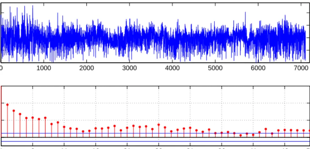
1 6 11 16 21 26 31 36 41 46 50 0 0.1 0.2 0.3 Lag 0 1000 2000 3000 4000 5000 6000 7000 0 500 1000 1500 2000
Fig 1.Up: Plot of the tree ring time series extracted from ca506.crn in ITRDB. Down: autocorrelation plot. The variance aggregation estimate for the Hurst index of the data yieldsHb(1)= 0.7182and the Hurst index for
the centered and squared data yieldsHb(2)= 0.7217; the local periodogram regression yieldsHb(1)= 0.7569and
b
H(2)= 0.7801respectively; the local Whittle estimate yields Hb(1)= 0.7024andHb(2)= 0.7061respectively.
contrast distribution constructed from fractional Gaussian noise, which makes comparison across
different data items (different m) more consistent. More technical explanations are given below.
LetFm(x) be the CDF of the randomδm. ThenFm(δm) follows exactly auniform distribution on
[0,1]. If {Xm(n)} were indeed generated by fractional Gaussian noise with true Hurst indexHbm(1),
then the empirical CDFFbm,Rin Step 4 is a good approximation ofFm. Therefore, if{Xm(n)}obeys
(38) as the fractional Gaussian noise does, andHbm(1) is a reasonable estimate, thenPm =Fbm,R(δm)
in Step 4 is expected to follow auniform distribution on [0,1] approximately. On the other hand, if
theδm computed from the data makes the distribution ofPm=Fbm,R(δm) skewed towards 1, then
this indicates that δm tends to be larger than δmr.
To account for the potential bias due to the estimation of the Hurst index, in Step 5 we replace our original data {Xm(n)} by a second contrast group {Xm∗(n)} made up of fractional Gaussian
noise sequences with similar lengths and Hurst indices. After repeating the same procedure on
this contrast group, we can then compare the distribution (histogram) of {Pm}obtained from the
original data with the distribution of {P∗
m} obtained from the contrast group.
These designs may be regarded as simulation-assisted statistical tests where the null hypothesis is the relation (38).
Now we describe the data we use. Thetree ring widthin chronological order has been identified as
one of the natural stationary time series data sets which exhibit long memory (see Mandelbrot and Wallis [58] and Pelletier and Turcotte [61]). Since the tree ring width is largely affected by
environ-mental factors, which is explored in dendrochronology (see Schweingruber [70]), it also reflects the
long-memory stationary fluctuation of the ecological systems. We shall use the data compiled by The
International Tree-Ring Data Bank (ITRDB,ftp://ftp.ncdc.noaa.gov/pub/data/paleo/treering/chronologies/)
collected from Africa, Asia, Australia, Canada, Europe, Mexico, South America and USA, stored
in the Standard Chronology File (*.crn) format. For example, Figure 1 displays the time series
extracted from the file ca506.crn in the data bank and its autocorrelation plot. We further select 17
the data according to the following criteria:
Criterion 1 The length of the time series is at least 300.
Criterion 2 The time series data is importable by the Tree-Ring Matlab Toolbox3 (data is usually
importable if there is no missing value).
Criterion 3 The estimated Hurst indexHbm(1) lies within the interval [0.6,0.9]4.
To be consistent, we also apply Criterion 1 and Criterion 3 for to the contrast group{X∗
m(n), n=
1, . . . , Nm}.
We shall use the following three popular estimators of Hurst index:
• Variance aggregation estimator;
• Local periodogram regression estimator (also known as GPH estimator);
• Local Whittle estimator.
For a description and empirical study of these estimators, see Taqqu et al. [78]. There are more
sophisticated estimators, for example, the wavelet-type estimators (see, e.g., Fa¨y et al. [34]). To minimize finite-sample bias, these methods typically involve complicated choice of some tuning pa-rameters. Since our study design has taken into account the potential bias of the estimator, we shall stick to the three more elementary estimators aforementioned. For the variance aggregation estima-tor and the local periodogram regression (GPH estimaestima-tor), we use the implementation by Chu Chen (http://www.mathworks.com/matlabcentral/fileexchange/19148-hurst-parameter-estimate, and we use the default parameter settings); For the local Whittle estimate, we use the
implementa-tion by Katsumi Shimotsu (http://shimotsu.web.fc2.com/Site/Matlab_Codes.html), in which
case we choose the frequency cutoff threshold to be [N2/3] with N being the length of the time
series).
Observations:
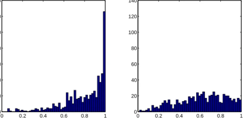
The graphs in the right-hand side of Figure 2, 3 and 4 are as expected, namely, corresponding
roughly to a uniform distribution. This indicates that the procedure described in the study is
reasonable. In fact, the median of P∗
m is roughly 50% as it should be (see Table 1). As mentioned
below, there may be a small bias when using the Local Periodogram Regression method (Figure 3
(right)). See also Taqqu and Teverovsky [77] for an empirical discussion of Whittle-type estimators.
Table 1 summarizes some key statistics of the analysis based on the three different estimators.
One can see that for all three estimators, the median of δm is consistently smaller than that of the
contrastδ∗
m. The median ofPmis significantly smaller than that of the contrastPm∗. Figure2,3and
4 plot the histograms of{Pm} and{Pm∗} obtained via the three different estimators. Their results
are similar: while {P∗
m} are roughly uniformly distributed as expected, the histogram of {Pm} is
severely skewed towards 1. The contrast in the skewness shows that the δm computed from the
tree ring data tends to be larger than the {δmr} computed from the fractional Gaussian noise. In
other words, in the case of tree ring data, the Hurst index doesnot tend to decrease as much after
squaring as the case of fractional Gaussian noise.
As mentioned in Remark4.1, if the Hurst index estimate is unbiased,P∗
m is expected to
approx-imately follow a uniform distribution on [0,1], so that the median is close to 1/2. However, the
3
http://www.ltrr.arizona.edu/~dmeko/toolbox.html
4
Ideally we want the selected data to be stationary and long-range dependent. When the estimate is close to 0.5, the data is likely to have short memory; when the estimate is close to 1, it is likely to be non-stationary.
Estimator Selected numberM Medianδm Medianδ∗m MedianPm MedianPm∗
Variance Aggregation 1250 0.0786 0.0104 80.50% 51.00%
Local Periodogram Regression 658 0.0921 -0.0204 86.25% 63.50%
Local Whittle 908 0.0496 -0.0162 80.50% 52.50%
Table 1
Analysis Summary
estimation bias of Hurst index could distort this uniformity. Indeed, in the Local Periodogram
Re-gression case, the median of P∗
m is 63.5%. But this is still in sharp contrast with the corresponding
median of Pm which is 86.25% and hence significantly larger. This indicates that the data is not
behaving like fractional Gaussian noise. Thus our design is effective despite the bias inherent in the estimation method.
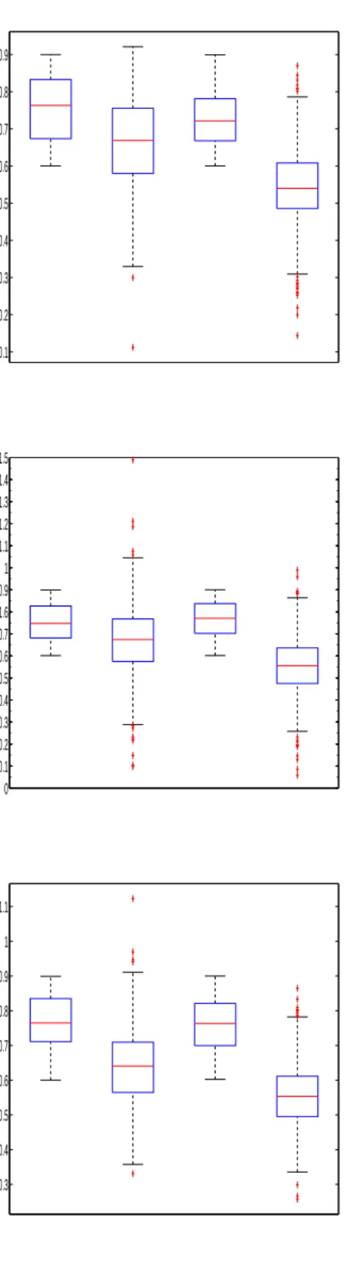
Remark 4.2. From the analysis above, we conclude that relation (38), or more generally (11), may not make good prediction on real-life data. We note, however, that the estimated Hurst index
b
Hm(2) of{Xm(n)2}tends to be somewhat smaller than the estimated Hurst indexHbm(1) of{Xm(n)},
although for the contrast group {X∗(n)} the decrease from Hbm(1)∗ to Hbm(2)∗ is more significant. See
Figure5. A possible explanation is that although {Xm(n)2}actually possesses rank 1 and thus has
the same Hurst index as {Xm(n)}, many of the {Xm(n)} may be close to a Gaussian (or linear)
process. So they tend to exhibit somewhat the relation (38) when the sample size is moderate. See
Bai and Taqqu [6] for an analysis of the interplay between the rank instability effect and the sample size.
Remark 4.3. As a reviewer pointed out, another explanation of the observations found in the study is that the data originally follows a model with a rank higher than 1, in which case squaring does not necessarily lead to a higher-order rank. Although this explanation is allowable in theory, it is less natural than the instability explanation. The reviewer’s explanation relies on assuming a special model: the transformation of a Gaussian or linear process with higher-order rank, while ours indicates that a slight perturbation makes the formula (38) unrealistic in practice.
5. STABILITY OF LIMIT THEOREMS UNDER WEAK DEPENDENCE
In this section, we demonstrate that the instability phenomenon appearing in the limit theorems under long memory does not typically occur in the short-memory case. This is important because it shows that the transformation considered as “perturbation” in the previous section usually does not make any qualitative difference in short-memory situations and hence may be safely negligible in large sample inference.
There are many ways to mathematically characterize weak dependence. For an introduction to various notions of weak dependence of stationary processes and corresponding limit theorems, we
refer to Doukhan [32]. In this section, we shall mainly look at the following three as examples:
(1) Fast-decaying mixing coefficients under strong mixing conditions;
(2) Fast decaying covariance function in Gaussian subordination model (Theorem5.2);
(3) Fast decaying physical dependence measure of Wu [81] in Bernoulli shift models.
The first is by far the most widely-used notion for weak dependence which applies to very general stationary processes. The second is mentioned due to its close connection to the considerations in
0 0.2 0.4 0.6 0.8 1 0 50 100 150 200 250 300 350 0 0.2 0.4 0.6 0.8 1 0 50 100 150 200 250 300 350
Fig 2.Histogram of {Pm}(left) v.s. {P∗
m} (right) from the Variance Aggregation Estimator
0 0.2 0.4 0.6 0.8 1 0 20 40 60 80 100 120 140 0 0.2 0.4 0.6 0.8 1 0 20 40 60 80 100 120 140
Fig 3. Histogram of {Pm} (left) v.s.{Pm∗}(right) from the Local Periodogram Regression
0 0.2 0.4 0.6 0.8 1 0 20 40 60 80 100 120 140 160 180 0 0.2 0.4 0.6 0.8 1 0 20 40 60 80 100 120 140 160 180
Fig 4. Histogram of {Pm} (left) v.s.{P∗
m} (right) from the Local Whittle Estimator
0.1 0.2 0.3 0.4 0.5 0.6 0.7 0.8 0.9 0 0.1 0.2 0.3 0.4 0.5 0.6 0.7 1.6 0.9 1 1.1 1.2 1.3 1.4 1.5 0.3 0.4 0.5 0.6 0.7 0.8 0.9 1 1.1
Fig 5.Top to bottom: variance aggregation estimator, local periodogram regression and local Whittle estimator. In each boxplot, from left to right: Hbm(1),Hb
(2) m ,Hb (1)∗ m andHb (2)∗ m . 21
Section2.1. The third is a convenient criterion under the Bernoulli shift framework which covers a wide range of concrete statistical models.
5.1 Strong mixing conditions
Suppose that {Y(n)} is a stationary process with E[Y(n)] = 0 and Var[Y(n)] = 1. Define the
σ-field Fb
a = σ{Y(n) : a ≤n ≤ b}, where −∞ ≤a ≤ b ≤+∞. Given two σ-fields A,B, one can
define the following measure of dependence
(39) α(A,B) = sup{|P(A∩B)−P(A)P(B)|: A∈ A, B∈ B}.
Then the α-mixing coefficient of {X(n}), first introduced in Rosenblatt [67], is defined as
αY(n) =α F−∞0 ,Fn∞
.
WhenαY(n)→0 asn→ ∞, we say that{Y(n)}isstrong mixing. If one assumes thatαY(n) decays
to zero fast enough together with some other regularity conditions, then a central limit theorem
for X(n) can be established. We state, as an example, the following central limit theorem due to
Ibragimov [49] and Herrndorf [43].
Theorem 5.1. If E|Y(n)|2+δ<∞ for someδ >0 and (40) ∞ X n=1 αY(n)δ/(2+δ)<∞, then 1 √ N [N t] X n=1 Y(n)−EY(n)⇒σB(t).
where B(t) is a standard Brownian motion, ⇒ stands for weak convergence in D[0,1], and
σ2 =
∞
X n=−∞
Cov[Y(n), Y(0)].
Now consider the transformation
X(n) =F(Y(n), . . . , Y(n−l)).
Let us compare αX and αY. Since X(n)∈ Fnn−l, it is easily deduced that for n > l, theα-mixing
coefficient of {X(n)} satisfies
(41) αX(n)≤αY(n−l).
The relation (41) means that the dependence measured by the α-mixing coefficient after the
per-turbing tranform F(·) cannot exceed that of the original process Y(n) (up to a fixed lag l). In
particular, relation (40) holds for αX(n).One then only needs E|X(n)|2+δ <∞ (which is the case
if F(·) has at most linear growth) for Theorem5.1to hold.
There are different mixing coefficients than α(n), obtained by modifying the measure of
depen-dence between the σ-fields in (39), for example, theφ-mixing coefficient defined through
φ(A,B) = sup{|P(A|B)−P(A)|: A∈ A, B∈ B, P(B)>0},
theρ-mixing coefficient defined through
ρ(A,B) = sup{Corr(X, Y) : X∈L2(A), Y ∈L2(B)},
and so on. In general, as long as a dependence measure m(·,·) is non-increasing with respect to
set inclusion and the mixing coefficient is defined as m(n) =m(F−∞0 ,F∞
n ), then a relation as (41)
always holds.
Hence, the central limit theorems under strong mixing conditions is robust against a transfor-mation perturbation.
5.2 Gaussian subordination
Let{Y(n)} be a stationary Gaussian process, and let
X(n) =F(Y(n), . . . , Y(n−l)).
When the covariance function ofY(n) decays fast enough, a central limit theorem always holds for
X(n). In particular, we have the following result which is a consequence of Ho and Sun [47]. Theorem 5.2. Suppose thatEX(n)2<∞ and
(42)
∞
X n=−∞
|Cov [Y(n), Y(0)]|<∞.
Then one has
1 √ N [N t] X n=1 X(n)−EX(n)f.d.d.−→ σB(t),
where B(t) is a standard Brownian motion and
σ2 =
∞
X n=−∞
Cov[X(n), X(0)].
Theorem5.2directly expresses the robustness of the central limit theorem against transformation
perturbation when the short memory condition (42) is imposed onY(n).
5.3 Bernoulli shift
Let {ǫi} be an i.i.d. sequence of random variables with mean 0 and variance 1. Consider the
Bernoulli shift model
(43) Y(n) =GY(ǫn, ǫn−1, . . .),
where GY is a non-random measurable function. This specification covers not only the causal
linear process (17), but also many nonlinear time series models obtained as solutions of difference
equations involvingǫi.
Wu [81] introduced the following so-called physical dependence measure for a process {Y(n)}
specified by (43). Letǫ∗
0 be a random variable independent of{ǫi}and having the same distribution
asǫ0. Define
(44) δ2X(n) =kGY(ǫn, . . . , ǫ1, ǫ0, ǫ−1, . . .)−GY(ǫn, . . . , ǫ1, ǫ∗0, ǫ−1, . . .)kL2 (Ω).
If (43) is interpreted as a nonlinear system with input{ǫn} and output{Y(n)}, then δ2Y(n) in (44)
measures the influence of the lag-ninput ǫ0 on the current outputY(n).
Withδ2Y(n), one can state the following central limit theorem, which is a consequence of Theorem 1 and 3 of Wu [81].
Theorem 5.3. Suppose that
∞
X n=1
δX2 (n)<∞.
(45)
Then one has
1 √ N [N t] X n=1 X(n)−EX(n)f.d.d.−→ σB(t), t≥0,
where B(t) is a standard Brownian motion, and
σ2 =
∞
X n=−∞
Cov[X(n), X(0)].
Remark 5.4. The criterion (45) is typically easier to check for a specific Bernoulli shift model
than the criteria based on strong mixing conditions (see Theorem5.1), while still providing
numer-ous statistical applications.
Now we consider the transformation perturbation. Let
X(n) =F(Y(n), . . . , Y(n−l+ 1)) =:GX(ǫn, ǫn−1, . . .).
We need to assume some smoothness condition (compare with the arguments of Claim2.11) on the
perturbation functionF(x1, . . . , xl). In particular, suppose that F(·) is Lipschitz, that is,
(46) |F(x1, . . . , xl)−F(y1, . . . , yl)| ≤CF l X
i=1
|xi−yi|
for some constant CF ≥0.
Settingǫn= (ǫn, . . . , ǫ1, ǫ0, ǫ−1, . . .) and ǫ∗n= (ǫn, . . . , ǫ1, ǫ∗
0, ǫ−1, . . .), one has by (46) that |GX(ǫn)−GX(ǫ∗n)| ≤CF
l−1
X i=0
|GY(ǫn−i)−GY(ǫ∗n−i)|.
Therefore, ifδ2X(n) andδ2Y(n) are the physical dependence measures of{X(n)}and{Y(n)} respec-tively, then δ2X(n) =kGX(ǫn)−GX(ǫ∗n)kL2(Ω)≤CF l−1 X i=0 δY2(n−i).
Hence if {Y(n)} satisfies the short memory condition
∞
X n=1
δ2Y(n)<∞,
then so does {X(n)}. This shows the robustness of Theorem 5.3 against a perturbation by any
Lipschitz transformation.
Remark 5.5. The proof of Theorem 5.3 is based on a martingale difference approximation method and resorts to the martingale difference central limit theorem. We note, however, that the martingale difference central limit theorem is itself not robust against transformation, since the martingale difference structure in general can be easily disturbed by a transformation. For example, in the stochastic volatility-type models, e.g., the LARCH(∞) model (Giraitis et al. [38]), the return sequence X(n) is a martingale difference, while |X(n)|can exhibit long memory (see Beran et al. [11], Chapter 4.2.8.).
Remark 5.6. Using similar arguments, one can show that the θ-weak dependence criterion (whose definition involves bounded Lipschitz transformation) introduced by Doukhan and Louhichi
[33], enjoys a robustness against bounded Lipschitz transformations.
6. CONCLUSION AND SUGGESTIONS
In this paper, we discussed the instability issue of Hermite rank and other related ranks appearing in limit theorems under long memory. We argued that a rank greater than 1 can be disturbed by a transformation and only a rank equal to 1 is stable. We provided empirical evidence supporting this argument. Such an instability feature has important statistical implications. In particular, assuming a higher-order rank when it is really not there may result in underestimating the order of fluctuation of the statistic of interest.
To address this issue we briefly indicate here some suggestions for performing valid inference.
As illustrated, particularly in Section 3, one may adopt the assumption that the rank is always 1,
regardless of any nonlinear transformation resulting from the statistical procedure. Here the rank
should be understood in a generalized sense, taking into account situations as (36). Some studies
have implicitly done so, although without giving an explanation (see, e.g., Beran [8] and Shao [72]).
Recently Beran et al. [12] designed a statistical test based on resampling to distinguish Hermite
rank 1 and a higher-order Hermite in the model (14).
Another appealing way out, is to redesign the statistical procedure in a way as to avoid using the fixed-rank limit theorems for inference directly. This may be achieved by combining re-sampling method (see, e.g, Hall et al. [42], Nordman and Lahiri [60], Zhang et al. [85]), Bai and Taqqu [5]),
together with suitable self-normalization technique (see, e.g., Shao [71] and Shao [72]). We refer
the reader to Jach et al. [50] Betken and Wendler [13] and Bai et al. [7] for approaches of this type.
APPENDIX A: NON-INSTANTANEOUS TRANSFORMATION OF THE GAUSSIAN
Let {Y(n)} be a standardized stationary long-memory Gaussian process with Hurst index H.
We extend here the discussion on instantaneous transformation (14) to the non-instantaneous
transformation
(47) X(n) =F Y(n), Y(n−1), . . . , Y(n−l),
whereX(n)∈L2(Ω) andlis a finite positive integer. Since the non-instantaneous case is much less treated in the literature, we shall introduce in this section the relevant results in Dobrushin and
Major [31], and show that the arguments developed in Section 2.1continue to be valid.
It is well-known that the GaussianY(n) admits the spectral representation (see, e.g., Dobrushin
and Major [31]) (48) Y(n) = Z (−π,π] einxWY(dx), 25
whereWY(dx) is a complex-valued Gaussian measure satisfying
(49) E|WY(dx)|2 =FY(dx)
andFY(·) is the spectral distribution5 ofY(n). ThenX(0) has following Wiener-Itˆo expansion (see
Dobrushin and Major [31], formula (6.1), or Janson [51], Theorem 7.61):
(50) X(0)−EX(0) = ∞ X m=1 Z ′′ (−π,π]m αm(x1, . . . , xm)WY(dx1). . . WY(dxm),
where the double prime′′ indicates the exclusion of the hyper-diagonals x
p =±xq in the multiple
stochastic integral. Hereαm(·)’s are a.e. unique complex-valued functions in satisfying
αm(x1, . . . , xk) =αm(−x1, . . . ,−xm), and ∞ X m=1 m!kαmk2L2(( −π,π]m,F⊗m Y ) <∞, where kαmkL2 ((−π,π]m,F⊗m Y ) 2 = Z (−π,π]m| αm(x1, . . . , xm)|2FY(dx1). . . FY(dxm).
The Hermite rank ofX(n) (or say the Hermite rank of F(·) with respect to {Y(n)}) is defined as
(51) infnm≥1 : kαmkL2((
−π,π]m,F⊗m Y )6= 0
o
,
The Hermite rank in (51) is also equal to (see Dobrushin and Major [31] Remark 6.3)
(52) infnm≥1 : Eh X(0)−EX(0)Y(n)mi6= 0 for some n∈Zo.
This should be compared to (7).
By Remark 6.1 of Dobrushin and Major [31], the a.e. unique functionαm(·) can further be chosen
to be continuous, which we shall assume throughout below. We are now ready to state the following
generalization of Theorem2.6, which follows from Dobrushin and Major [31] Theorem 3, Remark
6.3 and Remark 6.4.
Theorem A.1. Suppose thatX(n) =F(Y(n), . . . , Y(n−l)), and that the Hermite rank in the
sense of (51) is k, and that the Hurst index H of {Y(n)} satisfies
H >1− 1 2k.
Suppose also that αk(·) in (50) satisfies
(53) αk(0, . . . ,0)6= 0.
Then {X(n)} has long memory with Hurst index:
HF = (H−1)k+ 1∈ 1 2,1 . 5
Do not confuseFY in (49) withF in (47).