Economics Working Papers
3-2019
Working Paper Number 19007
Wild bootstrap for fuzzy regression discontinuity
designs: obtaining robust bias-corrected confidence
intervals
Yang He
Freddie Mac
Otávio Bartalotti
Iowa State University, [email protected]
Original Release Date: March 2019
Follow this and additional works at:
https://lib.dr.iastate.edu/econ_workingpapers
Part of the
Econometrics Commons
, and the
Economic Theory Commons
Iowa State University does not discriminate on the basis of race, color, age, ethnicity, religion, national origin, pregnancy, sexual orientation, gender identity, genetic information, sex, marital status, disability, or status as a U.S. veteran. Inquiries regarding non-discrimination policies may be directed to Office of Equal Opportunity, 3350 Beardshear Hall, 515 Morrill Road, Ames, Iowa 50011, Tel. 515 294-7612, Hotline: 515-294-1222, email
Recommended Citation
He, Yang and Bartalotti, Otávio, "Wild bootstrap for fuzzy regression discontinuity designs: obtaining robust bias-corrected confidence intervals" (2019).Economics Working Papers: Department of Economics, Iowa State University. 19007.
Wild bootstrap for fuzzy regression discontinuity designs: obtaining robust
bias-corrected confidence intervals
Abstract
This paper develops a novel wild bootstrap procedure to construct robust bias- corrected valid confidence
intervals (CIs) for fuzzy regression discontinuity designs, providing an intuitive alternative to existing
analytical methods. The CIs generated by this procedure are valid under conditions similar to the standard
analytical procedures used in the empirical literature. Simulations provide evidence that this new method is at
least as accurate as the analytical corrections when applied to a variety of data generating processes featuring
heteroskedasticity, endogeneity and clustering. Finally, we demonstrate its empirical relevance by revisiting
Angrist and Lavy (1999) analysis of class size on student outcomes.
Keywords
Fuzzy Regression Discontinuity, Robust Confidence Intervals, Wild Boot- strap, Average Treatment Effect
DisciplinesWild bootstrap for fuzzy regression discontinuity designs:
obtaining robust bias-corrected confidence intervals.
Yang He and Ot´
avio Bartalotti
First Draft: December, 2016.
This Draft: March, 2019.
Abstract
This paper develops a novel wild bootstrap procedure to construct robust bias-corrected valid confidence intervals (CIs) for fuzzy regression discontinuity designs, providing an intuitive alternative to existing analytical methods. The CIs generated by this procedure are valid under conditions similar to the standard analytical procedures used in the empirical literature. Simulations provide evidence that this new method is at least as accurate as the analytical corrections when applied to a variety of data generating processes featuring heteroskedasticity, endogeneity and clustering. Finally, we demonstrate its empirical relevance by revisiting Angrist and Lavy (1999) analysis of class size on student outcomes.
Key Words: Fuzzy Regression Discontinuity, Robust Confidence Intervals, Wild Boot-strap, Average Treatment Effect.
1
Introduction
Regression discontinuity (RD) designs are one of the leading empirical approaches in economics, political science, and public policy evaluation, being extensively used to estimate the causal effects of treatments or policies under transparent assumptions.1
The identification in RD designs exploits the fact that many policies and programs use a threshold based on a score, also called a “running variable” to assign treatment to individuals or firms. In that case, if the researcher credibly believes that subject’s position relative to the threshold is not related to unobserved characteristics driving the outcome of interest, we can attribute the differences between units slightly above and below the cutoff as caused by treatment alone. When the running variable does not
∗
He: Freddie Mac, 1551 Park Run Dr, McLean, VA 22102. Email: [email protected]. Bartalotti: Department of Economics, Iowa State University and IZA. 260 Heady Hall, Ames, IA 50011. Email: [email protected].
1Imbens and Lemieux (2008) and Lee and Lemieux (2010) provide reviews of this literature with many examples.
entirely determine the treatment, there are both treated and untreated units on each side of the cutoff, a situation referred to as the fuzzy RD design. Directly comparing the outcomes on both sides of the cutoff results in an intent-to-treat effect, and the average treatment effect at the cutoff can be recovered by taking the ratio of difference in outcomes and difference in treatment probabilities at the threshold, as in a Wald formulation of the treatment effect in the instrumental variable setting. Even when units are self-selected to treatment based on anticipated gains, Hahn et al. (2001) show that this ratio can be interpreted as the local average treatment effect (LATE) under proper assumptions.
The identification of RD designs occurs exactly at the cutoff, and in practice the treatment effect is typically estimated by fitting local linear models above and below the threshold, which are extrapolated to the exact point of discontinuity.23 The choice
of the bandwidth, h, in these nonparametric estimators, is an important econometric issue which controls the trade-off between bias and variance. One popular bandwidth selector proposed by Imbens and Kalyanaraman (2012) and extended by Calonico et al. (2014), henceforth “CCT,” minimizes the asymptotic mean squared error (AMSE) of the treatment effect estimator. However, this bandwidth selector has the form
h=Op(n−1/5), where nis the number of observations. As pointed out by CCT, the
AMSE-optimal bandwidth shrinks slowly enough that the leading bias term in the local polynomial estimators will be non-negligible, affecting the asymptotic distribution of the estimator. Consequently, the usual confidence intervals (CIs) for the RD treatment effects are invalid, and simulation studies on sharp RD designs in CCT, confirm that conventional CIs have empirical coverage well below their nominal levels.
CCT solve this problem by obtaining a valid estimate of the leading bias-term and re-centring the conventional point estimator. Furthermore, the additional variability introduced by the bias estimation needs to be considered when constructing CIs. This approach results in a bias-corrected point estimator which is asymptotically normal with weaker assumptions on the bandwidth. CIs based on this method are valid even when AMSE optimal bandwidths are used.
In this paper, a wild bootstrap procedure is proposed as an alternative to the analytical methods for bias-corrected robust inference for fuzzy RD designs. We theo-retically show that the new bootstrap procedure is asymptotically equivalent to CCT’s and provide simulation evidence that it performs well in finite samples. Compared with the analytical method, the bootstrap procedure is straightforward and does not require intensive derivations. Additionally, since the bootstrap is motivated by mimicking the true data generating process, it has the flexibility to accommodate dependent (clus-tered) data by adjusting the resampling algorithm accordingly. We demonstrate how the proposed bootstrap procedure can be applied to clustered data.
The wild bootstrap procedure exploits CCT’s theoretical insight by resampling from higher order local polynomials. In particular, the local linear models are estimated as usual for both outcome and treatment, resulting in a conventional biased estimator. To estimate the bias, additional local quadratic models are used, and the potentially correlated residuals on both the outcome and treatment equations serve as the “true”
2
See Fan (1992); Hahn et al. (2001) for a detailed discussion on local polynomial estimator properties and its use in RD designs.
3
data generating process (DGP) for the bootstrap. The bias of the conventional estima-tor is therefore known under this bootstrap DGP and can be calculated by averaging the error of the linear model’s estimates across bootstrap replications. Any remaining bias converges to zero at a faster rate, allowing the bias of the local linear model to be estimated. This approach is described in Algorithm 3.1 and the resulting bias-corrected estimator is shown to be asymptotically normal with mean zero in Theorem 3.1.
Following Bartalotti et al. (2017) we propose an iterated bootstrap procedure to account for the additional variability introduced by the bias correction: generate many bootstrap datasets from local quadratic models and calculate the bias-corrected esti-mate for each of them. The resulting empirical distribution of bias-corrected estimator is then used to construct CIs. This procedure is in line with CCT’s approach, where the variance of estimated bias term and the covariance between estimated bias and original point estimator are derived analytically. This complex adjustment to the orig-inal variance is automatically embedded in the iterated bootstrap. The bootstrap implementation is described in Algorithm 3.2, and the resulting CIs are shown to be asymptotically valid in Theorem 3.2.
Relative to Bartalotti et al. (2017), which developed a similar iterated bootstrap procedure for robust inference in special case of sharp RD designs, the current paper provides important generalizations in several dimensions. First, it connects the idea of bootstrapping IV models and adapts that to a more general fuzzy RD design. Second, its validity is extended and theoretically proved to general local polynomials and higher order of derivatives of interests, which could be used in the context of “Kink” RD designs, for example. Last, its flexibility and capability to accommodate clustered data is discussed and confirmed by simulation studies.
Concomitantly and independently, Chiang et al. (2017) proposed a multiplier boot-strap procedure that could be used in fuzzy RD and many related general settings based on a Bahadur representation of a general class of Wald estimators. Both the proce-dure and proofs in that paper differ from the ones proposed here and could potentially serve as alternatives in the cases covered by both approaches. Nevertheless, our pro-cedure benefits from its very intuitive nature, easy implementation and flexibility as exemplified in Section 5 when dealing with dependent (clustered) data.
The paper is organized as follows. Section 2 describes the basic fuzzy RD approach, its usual implementation, and the CCT’s robust inference method. Section 3 presents the proposed bootstrap procedures to estimate bias and construct confidence interval. Their asymptotic properties are discussed and summarized in two theorems. Section B provides simulation evidence that the bootstrap procedure effectively reduces bias and generates valid CIs. Implementation of the bootstrap to clustered data is discussed in Section 5. Section 6 demonstrates the applied relevance of this bootstrap procedure by applying it to the scholastic achievement data used by Angrist and Lavy (1999). Finally, Section 7 concludes.
2
Background
This section provides additional details of identification assumptions and traditional estimation methods in fuzzy RD designs. It also briefly introduces the robust
confi-dence interval proposed by CCT. Notations defined in this and following sections are consistent with CCT.
In a typical fuzzy RD setting, researchers are interested in the local causal effect of treatment at a given cutoff. For any unit i, (Xi, Ti, Yi) is observed, where Xi is
a continuous running variable which determines treatment assignment,Ti is a binary
variable which indicates actual treatment status and Yi is the outcome. In sharp
RD designs, the treatment actually received is the same as the assigned treatment, i.e., Ti = 1(Xi ≥ c), with c being the cutoff. In fuzzy RD designs, however, the
received treatment is not a deterministic function of running variableXi. Instead, the
probability Pr(Ti = 1 | Xi) is between zero and one in both sides but experiences a
sudden change at the cutoff. Without loss of generality, the cutoff c can be reset to zero. If assigned to treatment (Xi≥0), uniti’s actual treatment status and outcome
are represented by functions Ti(1) and Yi(1), otherwise Ti(0) and Yi(0). Thus the
observed treatment status and outcome are
Ti=Ti(0)1(Xi <0) +Ti(1)1(Xi ≥0)
Yi=Yi(0)1(Xi <0) +Yi(1)1(Xi≥0).
For each uniti’s outcome, either Yi(0) or Yi(1) is observed. The data itself is
unin-formative in terms of treatment effect because the counterfactual outcome could be arbitrary. However, under continuity and smoothness conditions onTi(0), Yi(0), Ti(1)
andYi(1) around the cutoff Xi = 0, it is possible to identify the treatment effect for
units just at the cutoff and the estimand of interest is
ζ= τY
τT
=E[Yi(1)|Xi= 0]−E[Yi(0)|Xi= 0] E[Ti(1)|Xi= 0]−E[Ti(0)|Xi= 0]
, (2.1)
where the symbol E represents the expectation and τY and τT represent the sharp
RD estimators, i.e., difference in expectations at the cutoff. Intuitively, this is a Wald estimator in the limit where the assigned treatment serves as an instrument. The reduced-form difference in expected outcome, τY, reveals the “intent-to-treat” (ITT)
effect. The treatment effect is recovered by dividing ITT effect by the difference in treatment probabilities. When the treatment effect is not constant across units, ζ
should be interpreted with caution. If treatment status is independent of treatment effects at the cutoff,ζ is the average treatment effect (ATE) at the cutoff. This as-sumption rules out self-selection based on anticipated gain. Hahn et al. (2001) show that under a less restrictive assumption that the running variable is independent of the joint distribution of treatment effect and treatment status at the cutoff, the LATE is identified.
Equation 2.1 presentsζas a ratio of two sharp RD estimators. Due to this symme-try, we use “Z” as a placeholder for either outcome variable Y or treatment variable
T to ease the notation. In addition, denote the conditional expectations µZ+(x) and µZ−(x), conditional variancesσZ2+(x) andσZ2−(x), theη-th order derivative of
as µZ+(x) = E[Zi(1)|Xi=x] µZ−(x) = E[Zi(0)|Xi=x] σZ2+(x) =V[Zi(1)|Xi =x] σ2Z−(x) =V[Zi(0)|Xi=x] µ(Zη+)(x) =d ηµ Z+(x) dxη µ (η) Z−(x) = dηµ Z−(x) dxη µ(Zη+) = lim x→0+µ (η) Z+(x) µ (η) Z−= lim x→0−µ (η) Z−(x)
where the symbolV(·) represents variance. The treatment effectζis nonparametrically estimable becauseµZ− andµZ+can be estimated consistently under Assumption 2.1,
which lists standard conditions in the fuzzy RD literature.4 (See, in particular, Hahn et al., 2001, Porter, 2003 and CCT.)
Assumption 2.1 (Behavior of the DGP near the cutoff ) The random variables
{Xi, Ti, Yi}ni=1form a random sample of sizen. There exists a positive numberκ0such
that the following conditions hold for all x in the neighbourhood (−κ0, κ0) around
zero: (a) The density of Xi is continuous and bounded away from zero at x; (b)
E[Zi4 | Xi = x] is bounded; (c) µZ−(x) and µZ+(x) are three times continuously
differentiable; (d)σ2Z−(x)andσ2Z+(x)are continuous and bounded away from zero; (e)
µT−(0)6=µT+(0).
Assumption 2.1(a) ensures that the number of data points arbitrarily close to the cutoff increases as the sample size grows. Part (c) imposes necessary smoothness condition to allow an approximation by second order polynomials. Parts (b) and (d) put standard restrictions on moments to ensure that the estimated local polynomials are well behaved. Part (e) requires that the treatment assignment as an instrument is valid, in the sense that it induces a first stage difference in treatment probability. In practice, local polynomial regression is widely used to estimate RD designs because of nice boundary properties.5 As an illustration, consider the local linear regression using kernel functionK(·) with a common bandwidth,h, used for both the outcome and the treatment at both sides of the cutoff. The estimated treatment effect is
ˆ ζ(h) = ˆτY(h) ˆ τT(h) =µˆY+(h)−µˆY−(h) ˆ µT+(h)−µˆT−(h) , (2.2) 4
Throughout the main text we focus on the case where the researcher implements a local linear model to estimateτZ and a quadratic model to approximate the bias term. The proofs presented in the appendix for the validity of the bootstraps proposed include the general case in which higher-order polynomials can be used to obtainτZ or a higher-order bias correction is implemented, e.g., Bartalotti (2018).
5See Fan and Gijbels (1996) for discussions on the boundary properties of local polynomial regression. See Gelman and Imbens (2018) for discussions on the choices of global and local polynomial regression and its order.
with ˆ µZ+(h) = arg min β0 min β1 n X i=1 1{Xi≥0}(Zi−β0−Xiβ1)2 1 hK Xi h ! ˆ µZ−(h) = arg min β0 min β1 n X i=1 1{Xi<0}(Zi−β0−Xiβ1)2 1 hK Xi h ! .
The conditional expectationsµZ+ and µZ− are consistently estimated by ˆµZ+(h)
and ˆµZ+(h) whenh→0.6 The asymptotic distribution of the quotient estimator ˆττˆY(h) T(h)
can be derived by applying the delta method. Let VZ be the asymptotic variance of
ˆ
τZ(h) andCY T be the asymptotic covariance between ˆτY(h) and ˆτT(h), i.e.,
√ nh(ˆτY(h)−τY) √ nh(ˆτT(h)−τT) d →N 0 0 , VY CY T CY T VT , √ nh( ˆζ(h)−ζ)→d N0, 1 τ2 T VY − 2τY τ3 T CY T+ τY2 τ4 T VT . LetV(h) =V( ˆζ(h)|X1, ..., Xn), then ˆ ζ(h)−ζ √ V(h) d
→N(0,1) and the CIs can be constructed as
ˆ
ζ(h)±q1−α/2V(h)1/2 (2.3)
whereq1−α/2is the 1−α/2 quantile of the standard normal distribution.
The above asymptotic distribution is valid only when bandwidth h shrinks fast enough such that the bias of ˆζZ(h) is negligible relative to
p
V(h). Formally, h =
op(n−1/5) is required. With a bandwidth of orderOp(n−1/5), Hahn et al. (2001) show
that the asymptotic distribution is normal but not centred at zero. Using (2.3) to construct CIs without considering this first-order bias in distributional approximation leads to coverage rates that differ from the nominal level. Imbens and Kalyanaraman (2012) develop plug-in bandwidth selector for RD estimators, which is optimal in the sense that AMSE of the point estimator is minimized.
Two different approaches are commonly adopted in empirical studies. One is undersmoothing. In this case, instead of using the AMSE-optimal bandwidth, re-searchers may want to choose a smaller bandwidth in order to meet the requirement of h = op(n−1/5). However, this often leads to a series of ad-hoc bandwidths
with-out theoretical basis. Another approach is bias correction, in which the leading bias is consistently estimated to remove the distortion of the asymptotic approximation. However, this approach does not perform well initially because the estimated bias in-troduces additional variability. CCT’s approach is based on bias correction, but derives an alternative asymptotic variance component for normalization so that the additional variability is accounted for.
For any bandwidth h → 0, the first-order bias of fuzzy RD estimator from local linear regression is E[ ˆζ(h)|X1, ..., Xn]−ζ=h2 1 τT BY(h)− τY τ2 T BT(h) (1 +op(1)), (2.4) 6
with BZ(h) = µ(2)Z+ 2 B+(h)− µ(2)Z− 2 B−(h).
The termsB+(h) and B−(h), explicitly defined in appendix, are observed quantities
that depend on the kernel, bandwidth and running variable. To explicitly calculate the first-order bias, one needs to estimate τZ, µ
(2)
Z+ and µ (2)
Z−. Among them τZ is
consistently estimated by the local linear regression with bandwidthh. CCT propose a local second-order regression with a (potentially) different bandwidth,b, to estimate the second order derivativesµ(2)Z+andµ(2)Z−. This produces the bias-corrected estimator
ˆ ζbc(h, b) = ˆζ(h)−∆(h, b), with ∆(h, b) =h2 1 ˆ τT(h) ˆ BY(h, b)− ˆ τY(h) ˆ τ2 T(h) ˆ BT(h, b) , ˆ BZ(h, b) = ˆ µ(2)Z+(b) 2 B+(h)− ˆ µ(2)Z−(b) 2 B−(h).
Notice that the bias ∆(h, b) is estimated with uncertainty. As a result, the variance of bias-corrected estimator ˆζbc(h, b) is different fromV(h). CCT propose a new formula
for the variance of bias-corrected estimator and use it for normalization: ˆ
ζbc(h, b)−ζ Vbc(h, b)1/2
d
→N(0,1), (2.5)
where Vbc(h, b) = V(h) +C(h, b) and C(h, b) captures the adjustment to variance
introduced by the bias-correction term. This distributional approximation is valid even when h = Op(n−1/5), as long as certain conditions on h and b are satisfied.
Assumption 2.2 specifies the bandwidth and kernel conditions assumed by CCT, which are also used in this paper.
Assumption 2.2 (Bandwidth and kernel) Let h be the bandwidth used to
esti-mate the local linear model and let b be the bandwidth used to estimate the local
quadratic model used to estimate the bias correction. Thennh → ∞, nb → ∞, and
n×min(h, b)5×max(h, b)2 → 0 as n → ∞. The kernel function K(·) is positive,
bounded, and continuous on the interval [−κ, κ] and zero outside that interval for
someκ >0.
Assumption 2.2 does not requirenh1/5→0. Instead, it only requires thatnh1/5b1/2→
0 whenh < bornb1/5h1/2→0 whenh > b. This assumption also allows for the vast
majority kernel functions commonly used in practice.
To simplify notation, letm= min(h, b) and define the scaled and truncated kernel functions
and
K+,b(x) =1bK(x/b)1{x≥0} K−,b(x) = 1bK(x/b)1{x <0}.
In the next section, a simple bootstrap procedure is proposed to construct robust CIs based on the insight provided by CCT’s bias-corrected estimator. This bootstrap procedure is straightforward in the sense that no derivation of analytical formulas for the bias, variance and covariance terms is required. The bias-corrected estimator and its confidence interval are numerically different from CCT’s but asymptotically equivalent.
3
Bootstrap Algorithm and Validity
In this section, two bootstrap algorithms are presented to obtain bias-corrected point estimator and its CIs in the fuzzy RD design, extending the results in Bartalotti et al. (2017). Their validity is justified in two theorems and proved in the appendix. The idea behind both algorithms is to use higher-order local polynomials to approximate the joint behaviour of (Xi, Ti, Yi) around the cutoff. These polynomials, together with the
empirical variance structure, serve as the “true” DGP in the bootstrap under which we evaluate the bias of the local linear estimator employed by the researcher when implementing RD. Assumption 2.2 guarantees that the estimated “true” DGP is close to the unknown DGP in the sense that distributional approximation derived from the “true” DGP is asymptotically valid. This can be best illustrated from the special case where the bandwidths used for estimatingτ and the bias are the same,h=b, which translates to the bandwidth conditionnb7 → 0 under Assumption 2.2. By the same
argument thath=op(n−1/5) is required for valid inference in a RD design estimated
by local linear regression,b=op(n−1/7) is required in a RD design estimated by local
quadratic regression.
Algorithm 3.1 consistently estimates the bias term.
Algorithm 3.1 (Bias estimation) Assume h and b are bandwidths as defined by Assumption 2.2.
Step1. Estimate local second order polynomials ˆgZ−and ˆgZ+with least squares using K−,bandK+,b for weights:
ˆ gZ−(x) = ˆβZ−,0+ ˆβZ−,1x+ ˆβZ−,2x2, gˆZ+(x) = ˆβZ+,0+ ˆβZ+,1x+ ˆβZ+,2x2 with ( ˆβZ−,0,βˆZ−,1,βˆZ−,2)0= arg min β0,β1,β2 n X i=1 (Zi−β0−β1Xi−β2Xi2)2K−,b(Xi) ( ˆβZ+,0,βˆZ+,1,βˆZ+,2)0= arg min β0,β1,β2 n X i=1 (Zi−β0−β1Xi−β2Xi2) 2K +,b(Xi). Let ˆ gZ(x) = ( ˆ gZ−(x) ifx <0 ˆ gZ+(x) otherwise
and calculate the residuals ˆεZi=Zi−ˆgZ(Xi) for all i.
Step2. Repeat the following steps B1 times to produce the bootstrap estimates
ˆ
η1∗(h), . . . ,ηˆB∗
1(h). For thekth replication:
2.1. Draw i.i.d. random variablese∗i with mean zero, variance one, and bounded fourth moments independent of the original data and construct
ε∗Zi= ˆεZie∗i,
Zi∗= ˆgZ(Xi) +ε∗Zi
for alli.
2.2. Calculate ˆµ∗Z+(h) and ˆµ∗Z−(h) by estimating the local linear model on the bootstrap data set usingK+,handK−,hfor weights:
ˆ µ∗Z−(h) = arg min µ min β n X i=1 (Zi∗−µ−βXi)2K−,h(Xi) ˆ µ∗Z+(h) = arg min µ min β n X i=1 (Zi∗−µ−βXi)2K+,h(Xi). 2.3. Save ˆζk∗(h) =µˆ ∗ Y+(h)−µˆ ∗ Y−(h) ˆ µ∗ T+(h)−µˆ ∗ T−(h). Step3. Estimate the bias as
∆∗(h, b) =B1 1 B1 X k=1 ˆ ζk∗(h)− ˆ gY+(0)−gˆY−(0) ˆ gT+(0)−gˆT−(0) . (3.1)
Algorithm 3.1 consists of three steps. The first step estimates the bootstrap DGP, which is captured by second order local polynomials. The second step creates a series of new samples through wild bootstrap and finds the traditional fuzzy RD estimate for each sample. Crucial for the procedure is that pairs of residuals are multiplied by the same realization of random numbere∗ to preserve the correlation between Yi and Ti.
The last step calculates the bias from local linear estimator in the bootstrap by defi-nition. Under Assumptions 2.1, 2.2 andB1 large enough, the procedure described by
Algorithm 3.1 consistently estimates the bias component, resulting in a bias-corrected estimator that has the same asymptotic distribution as in Equation (2.5). This con-clusion is formally given in Theorem 3.1.
Theorem 3.1 Under Assumptions 2.1 and 2.2,
ˆ
ζ(h)−∆∗(h, b)−ζ Vbc(h, b)1/2 →
dN(0,1), (3.2)
where∆∗(h, b)is defined by Equation (3.1).
Theorem 3.1 enables one to construct valid confidence interval in the form of ˆζ(h)−
∆∗(h, b)±Vbc(h, b)1/2. However, the termVbc(h, b) still needs to be calculated. The
bootstrap. In particular, the first layer bootstrap is designed to mimic the randomness due to sampling error and the second layer bootstrap, as described in Algorithm 3.1, is designed to estimate bias due to model misspecification. The additional variability introduced by the bias correction term will be automatically accounted for by this iterated bootstrap. The detailed procedure is given in Algorithm 3.2.
Algorithm 3.2 (Distribution) Assume h and b are bandwidths as defined by As-sumption 2.2 and Algorithm 3.1.
Step1. Estimate ˆgZ+ and ˆgZ− and generate ˆgZ(·) and the residuals ˆεZi just as in
Algorithm 3.1.
Step2. Repeat the following steps B2 times to produce bootstrap estimates of the
bias-corrected estimate. For thekth replication:
2.1. Draw i.i.d. random variablese∗i with mean zero, variance one, and bounded fourth moments independent of the original data and construct
ε∗Zi= ˆεZie∗i, Zi∗ = ˆgZ(Xi) +ε∗Zi.
for alli= 1, . . . , n.
2.2. Calculate ˆµ∗Z+(h) and ˆµ∗Z−(h) by estimating the local linear model on the bootstrap data set usingK+,handK−,hfor weights:
ˆ µ∗Z−(h) = arg min µ min β n X i=1 (Zi∗−µ−βXi)2K−,h(Xi), ˆ µ∗Z+(h) = arg min µ min β n X i=1 (Zi∗−µ−βXi)2K+,h(Xi).
2.3. Apply Algorithm 3.1 to the bootstrapped data set (X1, T1∗, Y1∗), . . . ,(Xn, Tn∗, Yn∗)
using the same bandwidthshandbthat are used in the rest of this algorithm but reestimating all of the local polynomials on the bootstrap data. Gener-ateB1new bootstrap samples and let ∆∗∗(h, b) represent the bias estimator
returned by Algorithm 3.1.
2.4. Save the estimator ˆζk∗(h) =µˆ
∗ Y+(h)−µˆ ∗ Y−(h) ˆ µ∗ T+(h)−µˆ ∗
T−(h), and its bias ∆
∗∗
k (h, b).
Step3. Defineζ∗=gˆgˆYT++(0)(0)−−ggˆˆTY−−(0)(0) and use the empirical CDF of ˆζ
∗ 1(h)−∆∗∗1 (h, b)− ζ∗, . . . ,ζˆB∗ 2(h)−∆ ∗∗ B2(h, b)−ζ
∗as the sampling distribution of ˆζ(h)−∆∗(h, b)−ζ.
Algorithm 3.2 also consists of three steps. The first step estimates the bootstrap DGP, which is captured by second order local polynomials. The second step creates a series of new samples, to which the Algorithm 3.1 is applied. The last step uses the empirical distribution of bias-corrected estimator to construct CIs. As before,
B2 is assumed large enough so that simulation error can be ignored. The validity of
Algorithm 3.2 is established in the following theorem. Theorem 3.2 Under Assumptions 2.1 and 2.2,
V∗( ˆζ∗(h)−∆∗∗(h, b))/Vbc(h, b)
and sup x Pr∗ " ˆ ζ∗(h)−∆∗∗(h, b)−ζ∗ V∗( ˆζ∗(h)−∆∗∗(h, b))1/2 ≤x # −Pr "ˆ ζ(h)−∆∗(h, b)−ζ Vbc(h, b)1/2 ≤x # →p0.
Theorem 3.2 enables one to construct CIs in the following form: ˆ
ζ(h)−∆∗(h, b)+ζ∗−( ˆζ∗(h)−∆∗∗(h, b))1−α/2,ζˆ(h)−∆∗(h, b)+ζ∗+( ˆζ∗(h)−∆∗∗(h, b))α/2
,
where all the terms with superscript∗are defined in Algorithm 3.2. Different from the analytical one, this CI is not centred at the bias-corrected point estimator.
Remark 3.1 The proposed bias correction differs from CCT’s analytical formula in finite samples. While the analytical bias is obtained by linearizing EhˆτY(h)
ˆ τT(h)− τY τT i and then only evaluating its first order terms, Algorithm 3.1 directly estimates EhτˆY∗(h)
ˆ τ∗ T(h) − τY∗ τ∗ T i
through bootstrap. Both methods consistently estimate the bias.
Remark 3.2 When the original treatment is binary, the bootstrap sample will no longer have binary treatment. Though it creates some difficulty for interpretation, it does not invalidate the estimation and inference because its conditional expectation and covariance with outcome variable remain unchanged.
Remark 3.3 The iterated bootstrap is less computationally intensive than it might initially appear due to two reasons. First, the wild bootstrap creates new residuals but leaves the regressors unchanged, which means the design matrices only need to be computed once even when they are repeatedly used in fitting local polynomials.7
Second, the number of data points actually used in estimation is a lot smaller than the full sample due to the local nature of the estimation.
4
Monte Carlo Simulations
This section summarizes the result of Monte Carlo experiments designed to evaluate the finite sample performance of the bootstrap procedures proposed in Section 3 relative to the existing analytical alternatives. The details about the data generating processes (DGP) used and implementation are provided in the appendix.
The conditional mean functions used in the simulations are similar to the ones used by CCT, adapted to the fuzzy RD context. For concreteness, the first mean function (DGP 1) is designed to match features of U.S. congressional election data from Lee (2008). The second mean function (DGP 2) matches the relationship between children mortality rate and county poverty rate from analysis of Head Start data in Ludwig and
7
To fit local polynomials is equivalent to estimate weighted least square, i.e., the estimated parameter is (X0KX)−1X0KY, where X is matrix of regressors and K is weighting matrix determined by kernel function. Both XandK are not affected by the bootstrap so one just need to compute (X0KX)−1X0K
once and then reuse it in the bootstrap calculations. Then each bootstrap replication just requires a single matrix-vector multiplication.
Miller (2007). The last mean function (DGP 3) is similar to the first one except for some coefficients. CCT motivates this as an attempt to generate plausible model with sizable distortion when conventional t-test is performed. The true treatment effects for these three models areζ1= 0.04, ζ2=−3.45, ζ3= 0.04, respectively.
To accommodate different endogeneity structures found in empirical data, we con-sider three cases. In the baseline case the treatment status is exogenous, i.e., there is no correlation between treatment assignment and the outcome. In the two endogenous cases the treatment status is correlated with unobserved characteristics which affect the outcome. This is modelled by the correlation,ρ, between the error terms on the outcome and treatment status equations as described in the appendix.
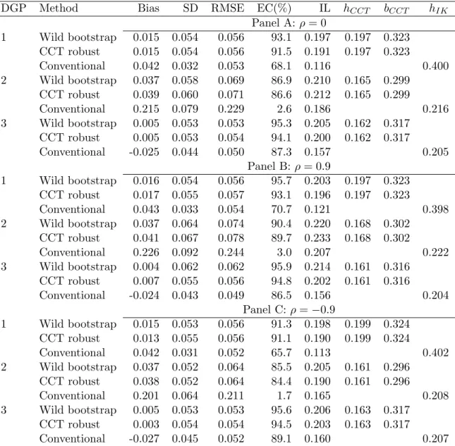
Besides the proposed bootstrap, two additional approaches are estimated for com-parison: CCT’s robust estimator and the conventional estimator. Simulation results are presented in Table 4.1. For the estimated treatment effect, its bias, standard error and root MSE are reported in the first three columns. For the CI, its empirical cov-erage and avcov-erage length are reported in the fourth and fifth columns. The last three columns list the average bandwidths used in the two robust methods (hCCT, bCCT)
and the conventional method (hIK).
The baseline case is listed in Panel A. The two robust methods, wild bootstrap and CCT’s approach, generate point estimates with very similar bias and standard errors. In contrast, the conventional approach reports 3-5 times larger bias. This is not surprising since the two robust methods explicitly correct the bias. The conventional method also fails to deliver a valid CI (coverage rates are 68.1%, 2.6% and 87.2% for the three DGPs respectively). Robust methods achieve improvements by reducing bias and increasing interval length. Except for DGP 2, they both generate intervals with empirical coverage close to the nominal level and the wild bootstrap performs well for DGPs 1 and 3. However, for DGP 2, even the robust methods report significant size distortion. This is because DGP 2 has great curvature around the cutoff and makes precise fitting challenging. Still, the two robust methods improve significantly on the coverage obtained by the conventional method (from 2.6% to around 87%) at the sacrifice of slightly longer intervals (from 0.186 to around 0.21).
Panels B and C present results when the treatment is endogenous, which is likely the primary reason to choose RD designs as the identification strategy. The case with positive (negative)ρis listed in Panel B(C). Again, the estimate from the conventional method has significantly larger bias than the two robust methods. As for CIs, the wild bootstrap and CCT’s approach work reasonably well in all cases. The conventional method performs significantly worse, with empirical coverage rate as low as 1.7%. The sign of correlation has little effect on the bias because the bias is caused by model misspecification rather than imperfect instrumental variable.
To summarize, the wild bootstrap approach proposed in this paper performs sig-nificantly better than the conventional method and is at least on par with the CCT’s analytical methods. This wild bootstrap procedure automatically accommodates var-ious types of covariance structure and thus is a simple alternative to obtain valid CIs in RD designs.
5
Extension: Clustered Data
This section explores the application of the bootstrap procedure to clustered data in RD designs and provides evidence for its usefulness. Clustered data are very common in empirical studies. Units within the same cluster are usually dependent and ignoring this dependence is likely to invalidate statistical inference. There is a vast literature on handling clustered data.8 In short, one can either explicitly estimate the dependence
structure with some additional specifications, such as random coefficient models, or account for the dependence after estimation, such as using cluster-robust variance estimator as discussed in Liang and Zeger (1986); Arellano (1987).
Cluster-robust variance estimators are very popular partly because they do not require assumptions on the dependence structure and partly because of its availability in most statistical softwares. Its validity is based on asymptotics when the number of clusters, G, grows to infinity, which is, unfortunately, not trivial to establish in nonparametric models. The main obstacle is that shrinking bandwidths is likely to destroy the dependence structure. For local polynomial regressions, Wang (2003) and Chen et al. (2008) point out that the existence of joint density of running variable and clustering variable ensures that cluster dependence vanishes asymptotically, not being captured by the usual approximations.9
Bartalotti and Brummet (2017) develop analytical approximations for the distri-bution and optimal bandwidth selector for the traditional RD estimator in a fixed-G
setting, sidestepping the issue. Recently available software provides options to take this dependence into consideration. Both therdrobust andRDD packages used in this paper offer the option to specify a clustering variable as explained by Calonico et al. (2017).
Naturally, a bootstrap approach could offer an alternative to the analytical approx-imations described. In fact, Cameron et al. (2008) provide a comprehensive survey of bootstrap methods and show that proper bootstrap procedures outperform the con-ventional cluster-robust variance estimator when the number of clusters is small (five to thirty).
To highlight the flexibility and robustness of the wild bootstrap procedure proposed in this paper, we revise the resampling algorithm to accommodate clustering and test its performance with pseudo clustered data. Following Brownstone and Valletta (2001) and Cameron et al. (2008), the wild bootstrap procedure for clustered data is quite straightforward: for units in the same cluster, their residuals are multiplied by the same random number drawn from the auxiliary distribution. For example,
Zgi∗ = ˆgZ(Xgi) + ˆεZgie
∗
g,
where e∗g, a random number from distribution with zero mean and unit variance, is shared by all units in the same group. For the purpose of simulation, it is assumed
8
See Wooldridge (2003); Cameron et al. (2011); Cameron and Miller (2015) for an overview on this topic. 9
A special case where this does not happen is that clustering occurs at the running variable level as discussed by Chen and Jin (2005).For example, in panel data where each individual are observed for multiple times and the running variable is at individual level, each individual is a cluster and will not vanish with shrinking bandwidth. Lee and Card (2008) consider another example in RD designs where clustering occurs at the running variable level and cluster-robust variance estimator is recommended for inference.
that errors in the outcome equation are clustered according to a random effect model, in particular,uygi=u∗yg+u∗yiwithg= 1,2, . . . , Gbeing a cluster indicator.
10
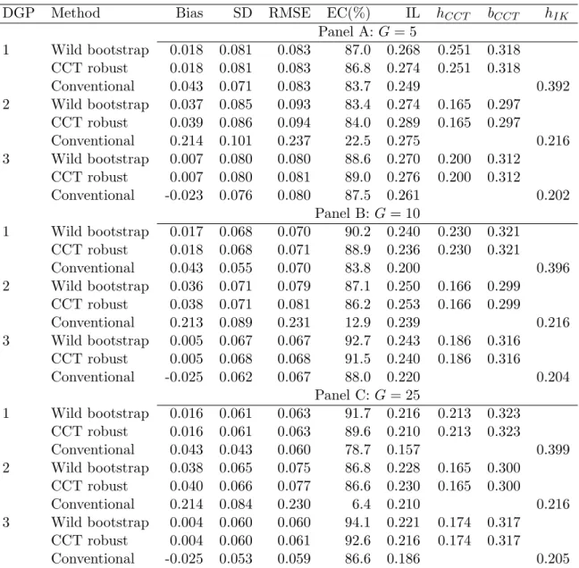
Simulation results for G = 5,10,25 are reported in Table 5.1.11 The wild
boot-strap approach consistently outperforms the conventional method, closely matching the coverage from CCT’s robust approach. This simple experiment shows that the wild bootstrap procedure proposed can also be easily applied to clustered data with slight adjustment to its resampling algorithm.
6
Empirical Illustration
In this section, we apply the bootstrap procedure to the data used in Angrist and Lavy (1999).12 In that paper, the effects of class size on scholastic achievement are estimated
using the “Maimonides’ rule” as instrument.
As described by Angrist and Lavy (1999) the “Maimonides’ rule” holds that the maximum class size is 40, and has been adopted by Israeli public schools to determine the division of enrollment cohorts into classes since 1969. Following this rule, when enrollment increases and passes multiples of 40, an additional class is required. Since the total enrollment is roughly evenly divided into all classes, an additional class causes a sudden drop in class sizes. Ideally, when the enrollment grows from 40 to 41, class size will drop by almost half. Because of student turnover and imperfect enforcement of this rule, the empirical data fits into a fuzzy RD design.
We consider the first discontinuity in class size for the 4thgrade. The sample used
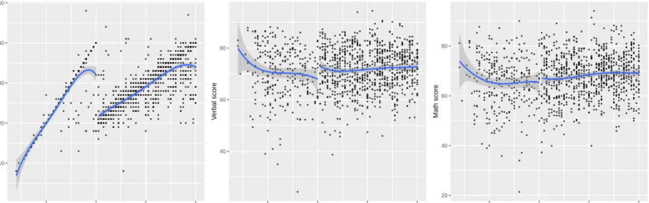
in this application includes 1164 classes from schools with enrollments no larger than 80. The outcome variables are average verbal and math test scores at class level. The discontinuities in class size and outcomes against enrollment are visualized in Figure 1. Each dot in these plots represents a class and the regression lines are fitted by fourth order polynomials. The shaded areas indicate CIs. The first plot clearly shows the discontinuity in class size, which is exploited for identification of the class size effect. The second plot suggests a discontinuity in average verbal score, but not as important as that in class size. The last plot does not provide much evidence for a discontinuity in average math score.
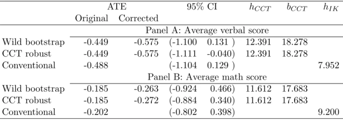
Three methods are applied to estimate the effect of class size on average ver-bal/math scores and results are shown in Table 6.1. The first column lists the original point estimates from local linear regression, which depends only on the bandwidth choice. The second column lists the bias-corrected point estimates based on bootstrap and analytical bias corrections. The estimates are very close to each other but differ meaningfully from the original estimates: the magnitude increases from 0.449 to 0.575 for average verbal score and 0.185 to 0.263∼0.272 for math score.
Consistent with what Figure 1 shows, only one out of three intervals for the ment effect on average verbal score excludes zero and all three intervals for the treat-ment on average math score include zero. The interval from wild bootstrap is wider
10The design ensures that the individual errors have the same standard errors as the baseline case pre-sented in Section B for easy comparison.
11Gdenotes the number of clusters on each side of the cutoff. 12
● ●● ● ● ● ● ● ● ● ● ● ● ● ●●● ●● ● ● ● ● ● ● ● ● ● ● ● ● ● ● ● ● ● ● ● ● ● ● ● ● ● ● ● ● ● ● ● ● ● ● ● ● ● ● ● ● ● ● ● ● ● ● ● ● ● ● ● ● ● ● ● ● ● ● ● ● ● ● ● ● ● ● ● ● ● ● ● ● ● ● ●● ● ● ● ● ● ● ● ● ● ●● ● ● ● ● ● ● ● ● ● ●● ● ● ●● ●● ● ● ● ●● ● ● ● ● ● ● ● ● ● ● ● ● ● ● ● ● ● ● ● ● ● ● ● ● ● ● ● ●● ● ●● ● ● ● ● ● ● ● ● ● ● ● ● ● ● ● ● ● ● ● ● ● ● ● ● ● ● ● ● ● ● ● ● ● ● ● ●● ● ● ● ●● ● ● ● ● ● ● ● ● ● ● ● ● ●● ● ● ●● ● ●● ● ● ● ● ● ● ● ● ● ● ● ● ● ● ● ● ● ● ● ● ● ● ● ● ● ● ● ● ● ● ● ● ● ● ● ● ● ● ● ● ● ● ● ●● ● ● ● ● ● ●● ● ● ● ● ● ● ● ●● ● ● ● ● ● ● ●● ● ● ● ● ● ● ● ● ● ● ● ● ● ● ● ● ●● ●● ● ● ● ● ● ● ● ● ● ● ● ● ● ● ● ● ● ● ● ●● ● ● ● ● ● ● ● ●● ● ● ● ● ● ● ● ● ● ● ● ● ● ● ● ● ● ● ● ● ● ● ● ● ● ● ● ● ● ●● ● ● ● ● ● ● ● ● ● ● ●● ● ● ● ● ● ● ●● ● ● ● ● ●● ● ● ● ● ● ● ● ● ● ● ● ● ● ● ● ● ● ● ● ● ● ● ● ● ● ● ● ● ● ● ● ● ● ● ● ● ● ● ●● ● ● ●● ● ● ● ● ●●● ● ● ● ● ● ● ●● ● ● ●● ● ● ● ● ● ● ● ● ● ● ● ● ● ● ●● ● ● ● ● ● ● ● ● ● ● ● ● ● ● ● ● ● ● ● ● ● ● ● ● ● ● ● ● ● ● ● ● ● ● ● ● ● ● ●● ●● ● ● ●● ●● ● ● ● ● ● ● ● ● ● ● ●● ●● ● ● ● ● ● ● ● ●● ●● ● ● ● ● ● ● ● ● ● ● ● ●● ● ● ● ● ● ● ● ●● ● ● ●● ● ● ● ● ● ●● ● ● ● ● ● ● ● ● ●● ● ● ● ● ● ● ● ● ● ●● ● ● ● ● ● ● ● ● ● ● ● ● ● ● ● ● ● ● ● ● ● ● ● ● ● ● ● ● ● ● ● ● ● ● ● ● ● ● ● ● ● ● ● ● ● ● ● ● ● ● ● ●● ● ● ● ● ●● ●● ● ●● ● ● ● ●● ● ●●●● ● ● ● ● ● ● ● ● ● ● ● ● ● ● ● ● ● ● ● ● ● ● ● ● ● ● ● ● ● ● ● ●● ● ● ● ● ● ●● ● ● ● ● ● ● ● ● ● ● ● ● ● ● ● ● ● ● ● ● ● ● ● ● ● ● ● ● ● ● ● ● ● ● ● ● ● ● ● ● ● ● ● ● ● ● ● ● ● ● ● ● ● ● ●● ● ● ● ● ● ● ● ● ● ● ● ● ● ● ● ● ● ● ● ● ● ● ● ● ● ● ● ● ● ● ● ● ● ● ● ● ● ● ● ● ● ● ● ● ● ● ● ● ●● ●● ● ● ● ● ● ● ● ● ● ● ● ●● ● ● ●● ● ● ● ● ● ●● ● ● ●● ● ●● ● ● ●● ● ● ● ● ● ● ● ● ●● ● ● ● ● ● ● ● ● ● ● ● ●● ● ● ● ● ● ● ● ● ●● ● ● ● ● ● ● ● ● ● ● ● ● ● ● ● ●● ● ● ● ● ● ● ● ● ●● ● ● ● ●● ● ● ● ● ● ● ● ● ● ● ● ● ●● ● ● ● ● ● ● ●● ● ● ● ● ● ● ● ●● ● ● ● ●● ● ● ● ● ● ● ● ● ● ● ● ● ● ● ● ● ● ● ● ● ● ●● ● ● ● ● ● ● ● ● ● ● ● ● ● ● ● ● ● ● ● ● ● ● ● ● ● ● ● ● ● ● ● ● ● ● ● ● ● ● ● ● ● ●● ●● ●● ● ● ● ● ● ● ● ● ●● ● ● ● ● ● ●● ● ● ●● ● ● ● ● ● ● ● ● ● ● ● ● ●● ● ● ● ●● ● ● ● ● ● ●● ● ● ● ●● ● ● ● ● ●● ● ●● ● ● ● ● ● ● ● ● ●● ● ● ● ● ● ● ● ● ● ● ● ● ● ● ●● ● ● ● ● ● ● ● ● ● ● ● ●● ● ● ●● ● ● ●● ● ● ●● ●● ● ● ● ● ● ●● ● ● ● ● ● ● ● ●● ● 10 20 30 40 50 20 40 60 80 Enrollment Class siz e ● ● ● ● ● ● ● ● ● ● ● ● ● ● ●● ● ● ● ● ● ● ● ● ● ● ● ● ● ● ● ● ● ● ● ● ● ● ● ● ● ● ● ● ● ● ● ● ●● ● ● ● ● ● ● ● ● ● ● ● ● ● ● ● ● ● ● ●● ● ● ● ● ● ● ● ● ● ● ● ● ● ● ● ● ● ● ● ● ● ● ● ● ● ● ● ● ● ● ● ● ● ● ● ● ● ● ● ● ● ● ● ● ● ● ● ● ● ● ● ● ● ● ● ● ● ● ● ● ● ● ● ● ● ● ● ● ● ● ● ● ● ● ● ● ● ● ● ● ● ● ● ● ● ● ● ● ● ● ● ● ● ● ● ● ● ● ● ● ● ● ● ●● ● ● ● ● ● ● ● ● ● ● ● ● ● ● ● ●● ● ● ● ● ● ● ● ● ●● ● ● ● ● ● ● ● ● ● ● ● ● ● ● ● ● ● ● ● ● ● ● ● ● ●● ● ● ● ● ● ● ● ● ● ● ● ● ● ● ● ● ● ● ● ● ● ● ● ● ● ● ● ● ● ● ● ● ● ● ● ● ● ● ● ● ● ● ● ● ● ● ● ● ● ●● ●● ● ● ● ● ● ● ● ● ● ● ● ● ● ● ●● ● ● ● ● ● ● ● ● ● ● ● ● ● ● ● ● ● ● ● ● ● ● ● ● ● ● ● ● ● ● ● ● ● ● ● ● ● ● ● ● ● ● ● ● ● ● ●● ● ● ●● ● ● ● ● ● ● ● ● ● ● ● ● ● ● ● ● ● ● ● ● ● ● ● ● ● ● ● ● ● ● ● ● ●● ● ● ● ● ● ●● ● ● ● ● ● ● ● ● ● ● ● ● ● ● ● ● ● ● ● ● ● ● ● ● ● ● ● ● ● ● ● ● ● ● ● ● ● ● ● ● ● ●● ● ● ● ● ●● ● ● ● ● ● ● ● ● ● ● ● ● ● ● ● ● ● ● ● ● ● ● ● ● ●● ● ● ● ● ● ● ● ● ● ●● ● ● ● ● ● ● ● ● ● ● ● ● ● ● ● ● ● ● ● ● ● ● ● ● ●● ● ● ● ● ● ● ●● ● ● ● ● ● ● ● ● ● ● ● ● ● ● ● ● ● ● ● ● ● ● ● ● ● ● ● ● ● ● ● ● ● ● ● ● ● ● ● ● ● ● ● ● ● ● ● ● ● ● ● ● ● ● ● ● ● ● ● ● ● ● ● ● ● ● ● ● ● ● ● ● ● ● ● ● ● ● ● ● ● ● ● ● ● ● ● ● ● ● ● ● ● ● ● ● ● ● ● ● ● ● ● ● ● ● ● ● ● ● ● ● ● ● ● ● ● ● ● ● ● ● ● ● ● ● ● ● ● ● ● ● ● ● ● ● ● ● ● ● ● ● ● ● ● ● ● ● ●● ● ● ● ● ● ● ● ● ● ● ● ● ● ● ● ● ●● ● ● ● ● ● ● ● ● ● ● ● ● ● ● ● ● ● ● ● ● ●● ● ● ● ● ● ● ● ● ● ● ● ● ● ● ● ● ● ● ● ● ● ● ● ● ● ● ● ● ● ● ● ● ● ● ● ● ● ● ● ● ● ● ● ● ● ● ● ● ● ● ● ●● ● ● ● ● ● ● ● ● ● ● ● ● ● ● ● ● ●● ● ● ● ● ● ● ● ● ● ●● ● ● ● ● ● ● ● ● ● ● ● ● ● ● ●● ● ● ● ● ● ● ● ● ●● ● ● ● ● ● ● ● ● ● ● ● ● ● ● ● ● ● ● ● ● ● ● ● ● ● ● ● ● ● ● ●● ● ● ●● ●● ● ● ● ●● ● ● ● ● ● ● ● ● ● ● ● ● ● ● ● ● ● ● ● ● ● ● ● ● ● ● ● ● ● ● ● ● ● ● ● ● ● ● ● ● ● ● ● ● ● ● ● ● ● ● ● ● ●● ●● ● ●● ● ● ● ● ● ● ● ● ● ● ● ● ● ● ● ● ● ● ● ● ● ● ● ● ● ● ● ● ● ● ● ● ● ● ● ● ● ● ● ● ● ● ● ● ● ● ● ● ● ● ● ● ● ● ● ● ● ● ● ● ● ● ● ● ● ● ● ● ● ● ● ● ●● ●● ● ● ● ● ● ● ● ● ● ● ● ● ● ● ● ● ●● ● ● ● ● ● ● ● ● ● ● ● ● ● ● ● ● ● ● ● ● ● ● ● ● ● ● ● ● ● ● ● ● ● ● ● ● ● ● ● ● ● ● ● ● ● ● ● ● ● ● ● ● ● ● ●● ● ● ● ● ● ● ● ● ● ● ● ● ● ● ● ● ● ● ● ● ● ● ● ●● ●● ● ● ● ● ● ● ● ● ● ● ● ● ● ● ● ● ● ● ● ● ● ● ● ● ● ● ● ● ● ● ● ●● ● ● ● ● ● ● ● ● ● ● ● ● ● ●● ● ● ● ● ● ● ● ● ● ● ● ● ● ● ● ● ● ● ● ● ● ● ● ● ● ● ●● ● 40 60 80 20 40 60 80 Enrollment V erbal score ● ●● ● ● ● ● ● ● ● ●● ● ● ● ● ● ● ● ● ● ● ● ● ● ● ● ● ● ● ● ● ● ● ● ● ● ● ● ● ● ● ● ● ● ● ● ● ● ● ● ● ● ● ● ● ● ● ● ● ● ●● ● ● ● ● ● ● ● ● ● ● ● ● ● ● ● ● ● ● ● ● ● ● ● ● ● ● ● ● ● ● ● ● ● ● ● ● ● ● ● ● ● ● ● ● ● ● ● ● ● ● ● ● ● ● ● ● ● ● ● ● ● ● ● ● ● ●● ● ● ● ● ● ● ● ● ● ● ● ● ● ● ● ● ● ● ● ● ● ● ● ● ● ● ● ● ● ● ● ● ● ● ● ● ● ● ● ● ● ● ● ● ● ● ● ● ● ● ● ● ● ● ● ● ● ● ● ● ● ● ● ● ● ● ● ● ● ● ● ● ● ● ●● ● ● ● ● ● ● ● ● ● ● ● ● ● ● ● ● ● ● ● ● ● ● ● ● ● ● ● ● ● ● ● ● ● ● ● ● ● ●● ● ● ● ● ● ● ● ● ● ● ● ● ● ● ● ● ● ● ● ● ● ● ● ● ● ● ● ● ● ● ● ● ● ● ●● ● ● ● ● ● ● ● ● ● ● ● ● ● ● ● ● ● ● ● ● ● ● ● ● ● ● ● ● ● ●● ● ● ● ● ● ● ● ● ● ● ●● ● ● ● ● ● ● ● ● ● ● ● ● ● ● ● ● ● ● ● ● ● ● ● ● ● ● ● ● ● ● ● ● ● ● ● ● ● ● ● ● ● ● ● ● ● ● ● ● ● ● ● ● ● ● ● ● ● ● ● ● ● ● ● ● ● ● ● ● ● ● ● ● ● ● ● ● ● ● ● ● ● ● ● ● ● ● ● ● ● ● ● ● ● ● ● ● ● ● ● ● ● ● ● ● ● ● ● ● ● ● ● ● ● ● ● ● ● ● ● ● ● ● ● ● ●● ●● ● ● ● ● ● ● ● ● ● ● ● ● ● ● ● ● ● ●● ● ● ● ● ● ● ● ● ● ● ● ● ● ● ● ● ● ● ● ● ● ● ● ● ● ● ● ● ● ● ● ● ● ● ● ● ● ● ● ● ● ● ● ● ● ● ●● ● ● ● ● ● ● ● ● ● ● ● ● ● ● ● ● ● ● ● ●● ● ● ● ● ● ● ● ● ● ● ● ● ● ● ● ● ● ● ● ● ● ● ● ● ● ● ● ● ● ● ● ● ● ● ● ● ● ● ● ● ● ● ● ● ●● ● ● ● ● ● ● ●● ● ● ● ● ● ● ● ● ● ●● ● ● ● ● ● ● ● ● ● ● ● ● ● ● ● ● ● ● ● ● ● ● ● ● ● ● ●● ● ● ● ● ● ● ● ● ● ● ● ● ● ● ● ● ● ● ● ● ● ● ● ● ● ● ● ● ● ● ● ● ● ● ● ● ● ● ● ● ● ● ● ● ● ● ● ● ● ● ● ● ● ● ● ● ● ● ● ● ● ● ● ● ● ● ● ● ● ● ● ● ● ● ● ● ● ● ● ● ● ● ● ● ● ● ● ●● ● ● ● ● ● ● ● ● ● ● ● ● ● ● ● ● ● ● ● ● ● ● ● ● ● ● ● ● ● ● ● ● ● ● ● ● ● ● ● ● ● ● ● ● ● ● ● ●● ● ● ● ● ● ● ● ● ● ● ● ● ● ● ● ● ● ● ● ● ● ● ● ● ● ● ● ● ● ● ● ● ● ● ● ● ● ● ● ● ● ● ● ● ● ● ● ● ● ● ● ● ●● ● ● ● ● ● ● ● ● ● ● ● ● ● ● ● ● ● ● ● ● ● ● ●● ● ● ● ● ● ● ● ●● ● ● ●● ● ● ● ● ● ● ● ● ● ● ● ● ● ● ● ● ● ● ● ● ● ● ● ● ● ● ● ● ● ● ● ● ● ● ● ● ● ● ● ● ● ● ● ● ● ● ● ● ● ● ● ● ● ● ● ● ● ● ● ● ● ● ● ● ● ● ● ● ● ● ● ● ● ● ● ● ● ● ● ● ● ● ● ● ● ● ● ● ● ● ● ● ● ● ● ● ●● ● ● ● ● ● ● ● ● ● ● ● ● ● ● ● ● ● ● ● ● ● ● ● ● ● ● ● ● ● ● ● ● ● ● ● ● ● ● ● ● ● ● ● ● ● ● ● ● ● ● ● ● ● ● ● ● ● ● ● ● ● ● ● ● ● ● ● ● ● ● ● ● ● ● ● ● ● ● ● ● ● ●● ● ● ● ● ● ● ● ● ● ● ● ● ● ● ● ● ● ● ● ● ● ●● ● ● ● ● ● ● ● ● ● ● ● ● ● ● ● ● ● ● ● ● ● ● ● ● ● ● ● ● ● ● ● ● ● ● ● ● ● ● ● ● ● ● ● ● ● ● ● ● ● ● ● ● ● ● ●● ● ● ●● ● ● ● ● ● ● ● ● ● ● ● ● ● ● ● ● ● ● ● ● ● ● ● ● ● ● ● ● ● ● ● ● ● ● ● ● ● ● 20 40 60 80 20 40 60 80 Enrollment Math score
Figure 1: Class size, average verbal and math scores
than that from robust analytical approach, suggesting that it is more conservative, which is in line with the simulations presented.
7
Conclusion
A new wild bootstrap procedure is proposed to correct bias and construct valid CIs in fuzzy RD designs. This new method provides an easy to implement alternative to the analytical results in Calonico et al. (2014) to obtain robust bias-corrected CIs, and is implemented through a novel iterated bootstrap that extends the results and procedures described in Bartalotti et al. (2017). This new procedure is proved to be theoretically valid and empirically supported by simulation studies, performing as well as analytical alternatives, including in the presence of clustered data which has not been previously studied. An empirical illustration is provided, confirming the procedure’s applied relevance.
Acknowledgements
This paper is derived from Yang He’s work on his doctoral dissertation while at Iowa State University. The authors are grateful to Gray Calhoun for his invaluable insight, help, and support during the preparation of the original version of this manuscript. We are also thankful to Brent Kreider, Cindy Yu for valuable comments.
References
Angrist, J. D. and V. Lavy (1999). Using maimonides’ rule to estimate the effect of class size on scholastic achievement. Quarterly Journal of Economics 114, 533–75.
Arellano, M. (1987). Practitioners’ corner: computing robust standard errors for within-groups estimators. Oxford Bulletin of Economics and Statistics 49, 431–34. Bartalotti, O. (2018). Regression discontinuity and heteroskedasticity robust standard
errors: Evidence from a fixed-bandwidth approximation. Journal of Econometric
Methods 8(1).
Bartalotti, O. and Q. Brummet (2017). Regression discontinuity designs with clustered data. In M. D. Cattaneo and J. C. Escanciano (Eds.), Regression Discontinuity
Designs: Theory and Applications (Advances in Econometrics), Volume 38, pp. 383–
420. Emerald Publishing Limited.
Bartalotti, O., G. Calhoun, and Y. He (2017). Bootstrap confidence intervals for sharp regression discontinuity designs. In M. D. Cattaneo and J. C. Escanciano (Eds.), Regression Discontinuity Designs: Theory and Applications (Advances in
Econometrics), Volume 38, pp. 421–53. Emerald Publishing Limited.
Brownstone, D. and R. Valletta (2001). The bootstrap and multiple imputations: harnessing increased computing power for improved statistical tests. Journal of
Economic Perspectives 15(4), 129–41.
Calonico, S., M. D. Cattaneo, M. H. Farrell, and R. Titiunik (2017). rdrobust: Software for regression-discontinuity designs. Stata Journal 17, 372–404.
Calonico, S., M. D. Cattaneo, and R. Titiunik (2014). Robust nonparametric confidence intervals for regression-discontinuity designs. Econometrica 82, 2295–326.
Cameron, A. C., J. B. Gelbach, and D. L. Miller (2008). Bootstrap-based improvements for inference with clustered errors. Review of Economics and Statistics 90, 414–27. Cameron, A. C., J. B. Gelbach, and D. L. Miller (2011). Robust inference with multiway
clustering. Journal of Business and Economic Statistics 29, 238–49.
Cameron, A. C. and D. L. Miller (2015). A practitioner’s guide to cluster-robust inference. Journal of Human Resources 50, 317–72.
Chen, K., J. Fan, and Z. Jin (2008). Design-adaptive minimax local linear regression for longitudinal/clustered data. Statistica Sinica, 515–34.
Chen, K. and Z. Jin (2005). Local polynomial regression analysis of clustered data.
Biometrika 92, 59–74.
Chiang, H. D., Y.-C. Hsu, and Y. Sasaki (2017). A unified robust bootstrap method for sharp/fuzzy mean/quantile regression discontinuity/kink designs.arXiv preprint
arXiv:1702.04430.
Davidson, R. and E. Flachaire (2008). The wild bootstrap, tamed at last. Journal of
Fan, J. (1992). Design-adaptive nonparametric regression. Journal of the American
Statistical Association 87, 998–1004.
Fan, J. and I. Gijbels (1996). Local polynomial modelling and its applications:
mono-graphs on statistics and applied probability 66, Volume 66. CRC Press, New York,
NY.
Flachaire, E. (2005). Bootstrapping heteroskedastic regression models: wild bootstrap vs. pairs bootstrap. Computational Statistics and Data Analysis 49, 361–76. Gelman, A. and G. Imbens (2018). Why high-order polynomials should not be used
in regression discontinuity designs. Journal of Business and Economic Statistics 0, 1–10.
Hahn, J., P. Todd, and W. Van der Klaauw (2001). Identification and estimation of treatment effects with a regression-discontinuity design. Econometrica 69, 201–09. Imbens, G. and K. Kalyanaraman (2012). Optimal bandwidth choice for the regression
discontinuity estimator. Review of Economic Studies 79, 933–59.
Imbens, G. W. and T. Lemieux (2008). Regression discontinuity designs: A guide to practice. Journal of Econometrics 142, 615–35.
Lee, D. S. (2008). Randomized experiments from non-random selection in us house elections. Journal of Econometrics 142, 675–97.
Lee, D. S. and D. Card (2008). Regression discontinuity inference with specification error. Journal of Econometrics 142, 655–74.
Lee, D. S. and T. Lemieux (2010). Regression discontinuity designs in economics.
Journal of Economic Literature 48, 281–355.
Liang, K.-Y. and S. L. Zeger (1986). Longitudinal data analysis using generalized linear models. Biometrika 73, 13–22.
Ludwig, J. and D. L. Miller (2007). Does head start improve children’s life chances? evidence from a regression discontinuity design.Quarterly Journal of Economics 122, 159–208.
MacKinnon, J. G. (2013). Thirty years of heteroskedasticity-robust inference. InRecent
advances and future directions in causality, prediction, and specification analysis, pp.
437–61. Springer.
MacKinnon, J. G. and H. White (1985). Some heteroskedasticity-consistent covariance matrix estimators with improved finite sample properties. Journal of
Economet-rics 29, 305–25.
Mammen, E. (1993). Bootstrap and wild bootstrap for high dimensional linear models.
Porter, J. (2003). Estimation in the regression discontinuity model. Unpublished
Manuscript, Department of Economics, University of Wisconsin at Madison, 5–19.
Wang, N. (2003). Marginal nonparametric kernel regression accounting for within-subject correlation. Biometrika 90, 43–52.
Wooldridge, J. M. (2003). Cluster-sample methods in applied econometrics. American
Table 4.1: Empirical coverage and average interval length
DGP
Method
Bias
SD
RMSE
EC(%)
IL
h
CCTb
CCTh
IKPanel A:
ρ
= 0
1
Wild bootstrap
0.015
0.054
0.056
93.1
0.197
0.197
0.323
CCT robust
0.015
0.054
0.056
91.5
0.191
0.197
0.323
Conventional
0.042
0.032
0.053
68.1
0.116
0.400
2
Wild bootstrap
0.037
0.058
0.069
86.9
0.210
0.165
0.299
CCT robust
0.039
0.060
0.071
86.6
0.212
0.165
0.299
Conventional
0.215
0.079
0.229
2.6
0.186
0.216
3
Wild bootstrap
0.005
0.053
0.053
95.3
0.205
0.162
0.317
CCT robust
0.005
0.053
0.054
94.1
0.200
0.162
0.317
Conventional
-0.025
0.044
0.050
87.3
0.157
0.205
Panel B:
ρ
= 0
.
9
1
Wild bootstrap
0.016
0.054
0.056
95.7
0.203
0.197
0.323
CCT robust
0.017
0.055
0.057
93.1
0.196
0.197
0.323
Conventional
0.043
0.033
0.054
70.7
0.121
0.398
2
Wild bootstrap
0.037
0.064
0.074
90.4
0.220
0.168
0.302
CCT robust
0.041
0.067
0.078
89.7
0.233
0.168
0.302
Conventional
0.226
0.092
0.244
3.0
0.207
0.222
3
Wild bootstrap
0.004
0.062
0.062
95.9
0.214
0.161
0.316
CCT robust
0.007
0.055
0.056
94.8
0.202
0.161
0.316
Conventional
-0.024
0.043
0.049
86.5
0.156
0.204
Panel C:
ρ
=
−
0
.
9
1
Wild bootstrap
0.015
0.053
0.056
91.3
0.198
0.199
0.324
CCT robust
0.013
0.055
0.056
91.1
0.190
0.199
0.324
Conventional
0.042
0.031
0.052
65.7
0.113
0.402
2
Wild bootstrap
0.037
0.052
0.064
85.5
0.205
0.161
0.296
CCT robust
0.038
0.052
0.064
84.4
0.190
0.161
0.296
Conventional
0.201
0.064
0.211
1.7
0.165
0.208
3
Wild bootstrap
0.005
0.053
0.053
95.6
0.206
0.163
0.317
CCT robust
0.003
0.054
0.054
94.5
0.203
0.163
0.317
Conventional
-0.027
0.045
0.052
89.1
0.160
0.207
Note: EC denotes empirical coverage and IL denote average interval length based on 5000 simulations; nominal coverage probabilities are 95% for each estimator. Sample size is 1000. The triangular kernel is used. The columnshCCT andbCCT list average optimal bandwidths following CCT’s method.The column hIKlists average optimal bandwidth minimizing MSE. The bootstrap approach usesB1= 500 replications to compute bias andB2 = 999 replications to obtain empirical distribution of bias-corrected estimator.
Table 5.1: Empirical coverage and average interval length (clustered data).
DGP
Method
Bias
SD
RMSE
EC(%)
IL
h
CCTb
CCTh
IKPanel A:
G
= 5
1
Wild bootstrap
0.018
0.081
0.083
87.0
0.268
0.251
0.318
CCT robust
0.018
0.081
0.083
86.8
0.274
0.251
0.318
Conventional
0.043
0.071
0.083
83.7
0.249
0.392
2
Wild bootstrap
0.037
0.085
0.093
83.4
0.274
0.165
0.297
CCT robust
0.039
0.086
0.094
84.0
0.289
0.165
0.297
Conventional
0.214
0.101
0.237
22.5
0.275
0.216
3
Wild bootstrap
0.007
0.080
0.080
88.6
0.270
0.200
0.312
CCT robust
0.007
0.080
0.081
89.0
0.276
0.200
0.312
Conventional
-0.023
0.076
0.080
87.5
0.261
0.202
Panel B:
G
= 10
1
Wild bootstrap
0.017
0.068
0.070
90.2
0.240
0.230
0.321
CCT robust
0.018
0.068
0.071
88.9
0.236
0.230
0.321
Conventional
0.043
0.055
0.070
83.8
0.200
0.396
2
Wild bootstrap
0.036
0.071
0.079
87.1
0.250
0.166
0.299
CCT robust
0.038
0.071
0.081
86.2
0.253
0.166
0.299
Conventional
0.213
0.089
0.231
12.9
0.239
0.216
3
Wild bootstrap
0.005
0.067
0.067
92.7
0.243
0.186
0.316
CCT robust
0.005
0.068
0.068
91.5
0.240
0.186
0.316
Conventional
-0.025
0.062
0.067
88.0
0.220
0.204
Panel C:
G
= 25
1
Wild bootstrap
0.016
0.061
0.063
91.7
0.216
0.213
0.323
CCT robust
0.016
0.061
0.063
89.6
0.210
0.213
0.323
Conventional
0.043
0.043
0.060
78.7
0.157
0.399
2
Wild bootstrap
0.038
0.065
0.075
86.8
0.228
0.165
0.300
CCT robust
0.040
0.066
0.077
86.6
0.230
0.165
0.300
Conventional
0.214
0.084
0.230
6.4
0.210
0.216
3
Wild bootstrap
0.004
0.060
0.060
94.1
0.221
0.174
0.317
CCT robust
0.004
0.060
0.061
92.6
0.216
0.174
0.317
Conventional
-0.025
0.053
0.059
86.6
0.186
0.205
Note: EC denotes empirical coverage and IL denote average interval length based on 5000 simulations; nominal coverage probabilities are 95% for each estimator. Sample size is 1000. The triangular kernel is used. The columnshCCT andbCCT list average optimal bandwidths following CCT’s method.The column hIKlists average optimal bandwidth minimizing MSE. The bootstrap approach usesB1= 500 replications to compute bias andB2 = 999 replications to obtain empirical distribution of bias-corrected estimator.