Cambridge Working Papers in Economics: 1877
NONPARAMETRIC ESTIMATION OF INFINITE ORDER REGRESSION
AND ITS APPLICATION TO THE RISK-RETURN TRADEOFF
Seok Young Hong Oliver Linton
5 June 2018
This paper studies nonparametric estimation of the infinite order regression E (𝑌𝑌𝑡𝑡𝑘𝑘|Ft-1), k ∈ ℤ with
stationary and weakly dependent data. We propose a Nadaraya-Watson type estimator that operates with an infinite number of conditioning variables. The established theories are applied to examine the intertemporal risk-return relation for the aggregate stock market, and some new empirical evidence is reported. With a bandwidth sequence that shrinks the effects of long lags, the influence of all conditioning information is modelled in a natural and flexible way, and the issues of omitted information bias and specification error are effectively handled. Asymptotic properties of the estimator are shown under a wide range of static and dynamic regressions frameworks, thereby allowing various kinds of conditioning variables to be used. We establish pointwise/uniform consistency and CLTs. It is shown that the convergence rates are at best logarithmic, and depend on the smoothness of the regression, the distribution of the marginal regressors and their dependence structure in a non-trivial way via the Lambert W function. The empirical studies on S&P 500 daily data from 1950-2016 using our estimator report an overall positive risk-return relation. We also .find evidence of strong time variation and counter- cyclical behaviour in risk aversion. These conclusions are attributable to the inclusion of otherwise neglected information in our method.
Cambridge Working Papers in Economics
Nonparametric estimation of in…nite order
regression and its application to the risk-return
tradeo¤
Seok Young Hong
yOliver Linton
zUniversity of Cambridge
This version: 5 June 2018
Abstract
This paper studies nonparametric estimation of the in…nite order regression
E(YtkjFt 1), k 2 Z with stationary and weakly dependent data. We propose
a Nadaraya-Watson type estimator that operates with an in…nite number of conditioning variables. The established theories are applied to examine the in-tertemporal risk-return relation for the aggregate stock market, and some new empirical evidence is reported. With a bandwidth sequence that shrinks the e¤ects of long lags, the in‡uence of all conditioning information is modelled in a natural and ‡exible way, and the issues of omitted information bias and spec-i…cation error are e¤ectively handled. Asymptotic properties of the estimator are shown under a wide range of static and dynamic regressions frameworks, thereby allowing various kinds of conditioning variables to be used. We estab-lish pointwise/uniform consistency and CLTs. It is shown that the convergence rates are at best logarithmic, and depend on the smoothness of the regression, the distribution of the marginal regressors and their dependence structure in a non-trivial way via the Lambert W function. The empirical studies on S&P 500 daily data from 1950-2016 using our estimator report an overall positive
We gratefully acknowledge helpful comments from John Aston, Xiaohong Chen, Jeroen Dalderop, Paul Doukhan, Jiti Gao, Shuyi Ge, Hayden Lee, Yuan Liao, Mikhail Lifshits, Richard Nickl, Alexei Onatski, Hashem Pesaran, Peter Phillips, Alessio Sancetta, Philippe Vieu, the Associate Editor and two anonymous referees. We also thank Alexey Rudenko for providing an original Russian photocopy of Sytaya (1974), Hyungjin Lee for translating the paper, and the ERC for providing …nancial support.
yStatistical Laboratory, Faculty of Mathematics, University of Cambridge; [email protected] zFaculty of Economics, University of Cambridge; [email protected]
risk-return relation. We also …nd evidence of strong time variation and counter-cyclical behaviour in risk aversion. These conclusions are attributable to the inclusion of otherwise neglected information in our method.
JEL Codes: C10; C58; G10.
1
Introduction
Conditional expectations are crucially important in …nancial economics, with pro-found implications in many applications including asset returns predictability, market e¢ ciency and risk management. One fundamental objective of the subject is to under-stand the dynamics of theexpected excess returns relative to its conditional variance, a measure of investment risk. Due to the latency of conditional expectations how-ever, there has been no universal agreement upon what is the best way to measure the objects. Di¤erence in the approaches to modelling and estimating the conditional mean and variance has led to disagreement on their measurement, and also, con‡icting empirical evidence on their intertemporal relation.
There are some fundamental di¢ culties in this estimation problem. First, there is a risk of misspeci…cation. Many existing approaches impose restrictive model as-sumptions, about which there is little direct empirical evidence. For instance, some studies have relied on parametric or semiparametric assumptions such as the ARCH or stochastic volatility models, where some high degree of structure is imposed on the re-turn generating process. Other studies have typically measured the conditional mean and conditional variance as projections onto some predetermined variables. These ap-proaches cannot be entirely justi…ed, since they are all necessarily prone to some degree of potential speci…cation error, see Linton (2009) and Escanciano, Pardo-Fernández and Van Keilegom (2017) for further discussions. Nonparametric modelling can be an e¤ective solution in this context. It is a well established practical tool for analyzing time series data; see for example Härdle (1990), Bosq (1996), or Fan and Yao (2003) for a comprehensive review. A major advantage of this approach is that the relation-ship between the explanatory variables under study, denoted by X = (X1; : : : ; Xd)
|
, and the response, sayY, can be modelled without assuming any restrictive parametric or linear structures. Stone (1980, 1982) showed that the best achievable convergence rate (in minimax sense) is n =(2 +d), where is the measure of smoothness and d is the dimension/order.
Choosing among a few conditioning variables introduce an element of arbitrariness into the econometric modelling of expectations. In particular, if information that investors consider important is neglected, then the corresponding estimates may be unreliable, Harvey (2001). Lettau and Ludvigson (2010) argued that contrasting con-clusions on the intertemporal risk-return relation are largely due to the prevalent use of only small amount of conditional information in modelling the conditional mean and variance. Indeed, such practice greatly restricts the dynamics for the variance process and may result in poor estimates, especially when the volatility is highly persistent, Linton and Perron (2003), Giraitis et al. (2008). For example, Pagan and Hong (1990) estimated the conditional moments with nonparametric estimates of E(rmt rf tjrm;t 1; : : : ; rm;t p) and Var(rmt rf tjrm;t 1; : : : ; rm;t p), wherermt rf t
denotes the excess market return and p = 1 or 4. Having ended up with a negative risk-return relation using their estimates, they conjectured that the conclusion may have been a¤ected by their use of only small, …nite number of conditioning variables. Noting the dependence of a GARCH process on the in…nite past history of returns (with declining weights), they wrote: “[A] nonparametric estimator of 2t appeals as a
solution ..., although the fact that it operates with only a …nite number of conditioning elements makes it unable to explicitly handle a GARCH type process. ... [O]ne might be able to establish consistency of the estimator [which deals with the in…nite depen-dence]. As far as we are aware, however, there are no current theorems that would justify such a conjecture."
1.1
Overview of Results
This paper comes up with an estimation method that e¤ectively addresses the afore-mentioned di¢ culties. We propose a Nadaraya-Watson type estimator that operates with an unrestricted number of conditioning variables. We derive large sample prop-erties of the estimator in extensive detail, thereby providing an answer to the long-standing question in the quotation above. With a bandwidth sequence that shrinks the e¤ects of long lags, the in‡uence of all conditioning information is modelled in a natural and ‡exible way, and both issues of omitted information bias and speci…-cation error are e¤ectively handled. It is worth noting that Harvey (2001) reported sensitivity of conditional expectations estimates on what type of conditioning vari-ables are used in modelling the expectations. He showed with examples how several parametric/nonparametric estimates (and the estimated risk-return relationship) may vary according to the choice of di¤erent predetermined conditioning information. In this paper, the established theories allow for various kinds of conditioning information.
This is achieved by letting our model assumptions cover a wide range of static and dynamic regressions frameworks. The latter includes the autoregression framework as a special case.
Linton and Sancetta (2009) tackled this estimation problem of in…nite order regres-sion in the autoregresregres-sions context. They established uniform almost sure consistency for stationary ergodic data without rates. In the conclusion, they conjectured that the limiting distribution of nonparametric estimators could be established, and that the rate of convergence would be logarithmic. Under strict cross-sectional and temporal i.i.d. assumption, Mas (2012) derived the convergence rate which is consistent with our results in the particular case they considered. Doukhan and Wintenberger (2008) studied the autoregressive model of order d=1 under a notion of weak dependence, and showed the existence of a stationary solution. This result was further studied in Wu (2011).
We make several contributions. First, we establish some theorems which answer several open questions posed in the literature. Speci…cally, we show pointwise consis-tency of our estimator under a set of mild regularity conditions. Further, we establish a central limit theorem for our estimator at a point under stronger conditions as well as for a feasibly studentized version of the estimator, thereby allowing pointwise in-ference to be conducted. Also, uniform consistency of the estimator is shown over a compact set of logarithimically increasing dimension. We prove that convergence rates depend on the smoothness of the regression function, the distribution of the marginal regressors and their dependence structure in a non-trivial way via the Lambert W function. We elaborate how each of those factors a¤ects the rate of convergence, and show that the best possible rate is, nonetheless, of logarithmic order in all cases. This re‡ects the di¢ culty of capturing nonparametrically the e¤ect of an in…nite number of lags.
Second, using our estimation method we found some empirical results that are limited in the existing literature. Our …ndings reveal new evidence on the dynamics of risk-return relation and its link with the macroeconomy, and add supporting evidence for explaining some major puzzles in …nancial economics. To elaborate, applying our methods on the US stock market we found a positive risk-return relation over around past 60 years overall which is what asset pricing models generally postulate, e.g. Merton (1973). In particular, the relation turns out to be highly positive and strongly statistically signi…cant in the recent 30 years period. Moreover, we also found that there has been a strong time variation and counter-cyclicity in risk aversion and in the conditional Sharp ratio. The time series of estimated risk aversion tend to move in the
opposite direction to the federal funds rate, a proxy for business cycle, with the sample correlation being 0:5708. The quarterly Sharpe ratio is also strongly counter-cyclical, rising over most periods of recessions. Indeed, when standard nonparametric method is employed instead, we noticed that these evidence is not revealed, or di¤erent con-clusions are reached. We believe our new empirical …ndings suggest an improvement in the econometric analysis, which is attributable to allowing for extended ‡exibility and the inclusion of otherwise neglected information in our method.
1.2
Technical challenges and sketch proposals for remedy
One major hurdle we inevitably face in the in…nite-dimensional setting is the non-existence of the usual notion of density p( ) for the regressor X. Since there is no -…nite Lebesgue measure in in…nite-dimensional spaces, the Lebesgue density (with respect to the in…nite product of probability measures) of the regressor cannot be de…ned via the Radon-Nikodym theorem. Consequently, standard asymptotic argu-ments for kernel estimators are no longer valid, for example, Bochner’s lemma whereby under suitable regularity conditions, for j = 1;21 hdE K j x X h = Z Kj(u)p(x uh)du !p(x)kKkjj as h!0 (1)
whereK is a multivariate kernel (see Section 2.2 below). So classical limiting theories in nonparametric literature cannot be readily extended.
We propose to adopt and apply some ideas from the functional regression literature. There is a vast literature on statistical research on functional data (typical examples include curves and images), which are in…nite-dimensional in nature. Ferraty and Vieu (2002) …rst studied the case where the regressor was function valued. Masry (2005) provided a rigorous treatment of nonparametric regression with dependent functional data in which X lies in a general semi-metric space, establishing the central limit theorem. Mas (2012) derived the minimax rate of convergence for nonparametric estimation of the regression function with strictly independent and identically distrib-uted covariates. Ferraty and Vieu (2006) detailed a number of extensions and gave an overview of nonparametric approaches in the functional statistics literature. Gee-nens (2011) gave an up-to-date accessible summary of the literature on nonparametric functional regression, and introduced the termcurse of in…nite dimensionality, which re‡ects the evident di¢ culties in nonparametric estimation of in…nite-dimensional
ob-jects due to extreme data sparsity. In the …nite dimensional case more smoothness can mitigate completely the slower rate of convergence caused by dimensionality, but in the in…nite dimension case, additional smoothness can only mildly improve the convergence rate of estimators. We discuss in the next section the di¤erence between the functional data framework and our discrete time framework.
There is another potential problem that may arise speci…cally in the in…nite dimen-sional setting. In the dynamic regression framework, the regressor vector Xt includes
the in…nite lags of a variable Zt, say the response variable. Consequently, the class
of mixing type assumptions, a popular notion of dependence in the econometrics lit-erature, is generally not applicable. This is because measurable functions of Xt will
depend upon the in…nite time-lags ofZt, and are not mixing in general, see e.g.
David-son (1994). Therefore, in order to establish asymptotic theories, an alternative set of dependence assumptions should be imposed on the data generating process. We defer further discussions to Section 2.1 below.
Lastly, for notations, we de…ne an ' bn by an = bn +o(1), and cn dn by
equivalence of order between the two sequences cn and dn. Also, f g means there
exists some constant c > 0 such that limn!1f(n)=g(n) c. The term ‘stationarity’ is taken to mean strict stationarity. Throughout,C (orC0,C00) refers to some generic constant that may take di¤erent values in di¤erent places unless de…ned otherwise.
2
Some Preliminaries
Consider the regression model
Y =m(X) +"; (2)
where the regressor X = (X1; X2; : : : :)
|
is a random element taking values in some sequence space S, the response Y is a real-valued variable, and the stochastic error " is such that E("jX) = 0 a.s. The objective is to estimate the Borel function
m( ) = E(YjX = ) (3)
based onnrandom samples observed from a strictly stationary data generating process
f(Yt; Xt)2R Sgt2Z having some weak dependence structure. Details on the
assump-tions are given in Section 2.1 below.
This setting is related to the usual framework adopted for functional data, which has been widely studied by statisticians, see Ramsey and Silverman (2002), Aneiros, Bongiorno, Cao and Vieu (2017). Recently, successful attempts have been made to
develop theories for nonparametric inference in the functional statistics literature; Ferraty and Romain (2010) gives a comprehensive review. A major issue in this …eld of research lies in extending the statistical theories applicable toRdto function spaces.
In this literature, attention is usually on smooth functions that are approximated and reconstructed from …nely discretised grids on some compact interval. In contrast, the setup in our model (2) can be viewed as looking at a countable number of discrete observations. Such a di¤erence is re‡ected by the fact that the observed data is taken to be a discrete process X = (Xs) with unbounded s 2 Z+ so that S = ffjf :
N ! Rg, rather than X = (X(s)) with s 2 [0; T]k so that S = ffjf : [0; T]k
Rk ! Rg, e.g. curves if k = 1, images if k 2. The discrete nature of our setting has several fundamental distinctive features that allow us to look further into many speci…c practical issues.
An immediate consequence of our framework is that the tuning parameter can be imposed on each and every dimension, allowing one to control the marginal in‡uence of the regressors. For instance when it is sensible to postulate that the in‡uence of distant covariates is getting monotonically downweighted, one may set the marginal bandwidths to increase in the lag horizon so as to impose higher amount of smoothing. Depending on the nature of the regressor, S may be taken as the space of all in…nite real sequences R1 := Q1
j=1Rj formed by taking Cartesian products of the reals, or
its various linear subspaces such as `1, `p, c. We propose to take S = R1 so as to
refrain from imposing any prior restrictions with regard to the choice of the regressor; for example, taking S to be the space of bounded sequences excludes the possibility of having regressors with in…nite support (e.g. Gaussian process).
2.1
Dependence structure and leading examples
A distinctive characteristic of time series data is temporal dependence between ob-servations. In the nonparametric time series literature, Rosenblatt (1956)’s -mixing has been the de facto standard choice due to it being the weakest among the class of mixing-type asymptotic independence conditions. Roussas (1990) established point-wise and uniform consistency of the local constant estimator under this condition, respectively, while Fan and Masry (1992) established asymptotic normality. The -mixing condition has also been widely used in the context of dependent functional observations, see for instance Ferraty et al. (2010), Masry (2005), and Delsol (2009). Definition 1. A stochastic processfZtg1t=1de…ned on some probability space ( ;F; P)
is called -mixing (cf. ‘jointly’ -mixing if Zt isRd-valued, with d2(1;1]) if
(r) := sup
A2Ft
1;B2Fr1+t
jP(A\B) P(A)P(B)j
is asymptotically zero as r ! 1, where Fb
a is the -algebra generated by fZs;a
s bg. In particular, we say the process is algebraically (respectively exponentially)
-mixing if there exists some c; k > 0 such that (r) cr k (respectively if there
exists some ; & >0 such that (r) exp( &r )).
The popularity of the -mixing condition (note the modi…er - will occasionally be omitted if no confusion is likely) in the literature stems from the fact that it is easy to work with, see e.g. Doukhan (1994), Rio (2000) for a comprehensive survey. However, there are several limitations that have been pointed out in the literature. First, it is a rather strong technical condition that is hard to verify in practice. Second, some basic processes are not mixing. e.g. AR(1) with Bernoulli innovations, Andrews (1984).
We turn to our setting. In the static regression case it is appropriate to assume the mixing condition, but in the dynamic case this condition is not generally applicable as we now explain. Recall that the object of estimation is the conditional meanE(YtjF),
cf. (2), where the information set F is determined by the nature of the conditioning variables. There are two leading cases: the …rst case is the static regression where the information set is taken to mean (Xjt;j = 1;2; : : :), the -algebra generated
by the exogenous marginal regressors. The second case is the autoregression, where Xtj =Yt j for all j, in which case F =Ft 1 represents (Ys;s t 1), the -algebra
generated by the sequence of lags of the response (Ys)s t 1. In fact, as for the latter
framework we may consider a more general setup, i.e. a dynamic regression, where the information set is taken to be F = (Xjs; Ys; s t 1) for some j. Details are
formally given in Assumptions A below.
In the static regression case the usual joint -mixing condition can be assumed on the sample datafYt; Xtg as is usually done; since marginal regressors are observed at
the same time t: Xt = (X1t; X2t; : : :)
|
, assuming joint dependence does not require additional adjustments. Indeed, it can be easily shown that joint mixing implies both marginal component processes and any measurable function thereof are mixing.1 In this paper, we do not necessarily require independence between component processes
fXjtg, j = 1;2; : : :; later we specify to what extent some dependence can be allowed
1The converse is not necessarily true unless the marginal processes are independent to each other,
(see Assumption C). It will turn out that the requirement is mild and allows su¢ cient generality in application.
Moving on to the dynamic regression setting, since the regressors are taken to be the lags of the response and/or a covariate, measurable functions of Xt depend on
in…nite time-lags and hence arenot necessarily mixing.2 Therefore an alternative set of dependence conditions is necessary to establish asymptotic theories for the second framework. We adopt the notion of near epoch dependence due to Ibragimov (1962) for the dynamic regression setting and deal with two leading cases separately.
Definition 2. A stochastic processfZtg1t=1de…ned on some probability space ( ;F; P)
is called near-epoch dependent or stable in L2 with respect to a strictly stationary
-mixing process f tgif the stability coe¢ cients v2(r) :=EjZt Zt;(r)j2 is asymptotically
zero as r! 1, where Zt;(r) = r( t; : : : ; t r+1)for some Borel function r :Rr !R.
A process that is near epoch dependent on a mixing sequence is in‡uenced pri-marily by the “recent past” of the sequence and hence asymptotically resembles its dependence structure; see e.g. Billingsley (1968), Davidson (1994), or Lu (2001) for details. Andrews (1995) established uniform consistency of kernel regression estima-tors under near epoch dependence conditions. Following the usual convention, e.g. Bierens (1983), we shall take r( t; : : : ; t r+1) E(Ztj t; : : : ; t r+1). In Section 2.3
it will be shown that under suitable conditions similar asymptotic theories can be derived for both static and dynamic regression frameworks.
2.2
Local Weighting
In this section we …x the notions of local weighting and the measure of closeness between the data objects. Let K : [0;1) ! [0;1) =: R+ be a univariate density
function and for an element u of a normed sequence space, let
K(u) :=K(kuk): (4)
In our setting the properties of K are crucially important. We now group the kernel functions into three subcategories depending on how they are generated. The …rst two, referred to as Type-I and Type-II kernels in Ferraty and Vieu (2006) generalize the usual ‘window’kernels and monotonically decreasing kernels in …nite dimension,
2Except for some very special cases; Davidson (1994, Theorem 14.9) gives a set of technical
respectively. Both types of kernels are continuous on a compact support [0; ]. Definition 3. A function K : [0;1) ! [0;1) is called a kernel of type I if it integrates to 1, and if there exist real constants C1; C2 (with 0< C1 < C2) for which
C11[0; ](u) K(u) C21[0; ](u); (5)
where is some …xed positive real number. A function K : [0;1)! [0;1) is called
a kernel of type II if it satis…es (5) with C1 0, and is continuous on [0; ] and
di¤erentiable on (0; ) with the derivative K0 that satis…es
C3 K0(u) C4
for some real constants C3; C4 such that 1< C3 < C4 <0.
The de…nition above suggests that the uniform kernel on [0; ] is a type-I kernel, and the Epanechnikov, Biweight and Bartlett kernels belong to the class of Type-II kernels. Some of those with semi-in…nite support, for example (one-sided) Gaussian, are covered by the last group, which we will call the Type-III kernels.
Definition 4. A function K : [0;1)![0;1)is a kernel of type III if it integrates
to 1, and if it is of exponential type; that is, K(r)/exp(Cr ) for some and C.
2.3
Small deviations
The small ball (or small deviation) probability plays a crucial role in establishing the
asymptotic theory. Let S be a sequence space equipped with some norm k:k; then the small ball probability of anS -valued random element Z is a function de…ned as
'z(h) := P(kz Zk h); (6)
where h 2 R+: The probability is called centered if z = 0 (in which case we write
'(h)) and shifted (with respect to some …xed point z 2 S nf0g) if otherwise. The relation between the two quantities cannot be explicitly speci…ed in general, and will be given in terms of the Radon-Nikodym derivative (See Assumption D2 below).
The name small ball stems from the fact that we are interested in the asymptotic behaviour of 'z(h) as h tends to zero. The function can be thought of as a measure for how much the observations are densely packed or concentrated around the …xed
point z with respect to the associated norm and the reference distance h. From the de…nition it is straightforward to see that 'z(h) ! 0 as h ! 0, and that n'z(h)
is an approximate count of the number of observations whose in‡uence is taken into account in the smoothing procedure. WhenZ is a continuous random vector of …xed dimension d with densityp( )>0, it can be readily shown that the shifted small ball probability (with respect to the usual Euclidean norm) is given by
'z(h) = Vdhdp(z) = O(hd); (7)
where Vd= d=2= (d=2 + 1) is the volume of thed-dimensional unit sphere.
However, when Z takes values in an in…nitedimensional normed space, it is di¢ -cult to specify the exact form of the small ball probability, and its behaviour varies depending heavily on the nature of the associated space and its topological structure. Due to the non-equivalence of norms in in…nite dimensional spaces, it is intuitively clear that the “speed”at which'z(h)converges to zero is a¤ected by the choice of the norm k:k. Nonetheless, a rapid decay is expected in general irrespective of the choice of the norm due to the extreme sparsity of data in in…nite-dimensional spaces.
One possible example ofS is(`r;k:kr), the space ofr-th power summable sequence
equipped with the`r-norm; the centred small ball behaviour of sums of weighted i.i.d.
random variables is widely studied in the literature, see for example Borovkov and Ruzankin (2008) and references therein. In this work here, we will focus our main attention on the case ofr = 2 (and take k:k to meank:k2 unless speci…ed otherwise).
Nevertheless, we note that the results derived in this paper can be extended to the case of r >2 as long as the regularity conditions are adjusted appropriately.
Writing the expected value of the kernel in terms of the small ball probability EK z Z h =EK kz Zk h = Z K(u) dPkz Zk=h(u) = Z K(u) d'z(uh); (8)
we are able to bypass the di¢ culties mentioned in the introduction, and to establish the convergence of the integrals without requiring the existence of the Lebesgue density.
Lemma 1 Ferraty and Vieu (2006, Lemma 4.3 & 4.4). Suppose k:k is some
semi-norm de…ned on a function space. If K is type-I, then it satis…es
C1j 1 'z(h )
Z
0
where C1; C2 >0 are as de…ned in De…nition 3. When the kernel K is type-II, if 9 "0 >0; C5 >0 s.t. 8" < "0; Z " 0 'x(u)du > C5"'x(") (10) then we have C6j 1 'z(h ) Z 0 Kj(v) d'z(vh) C7j; j = 1;2 (11)
where the constants C6 = C5C4 and C7 = sups2[0; ]K(s) are strictly positive.
Under the regularity conditions of Lemma 1, (9) and (11) hold for everyh >0, so it follows that for any kernels of type-I and II:
Corollary 1 If the kernel K is either type-I or type-II, then for j = 1;2 we have 1
'z(h )E K
j z Z
h ! j as h!0
+; (12)
where 1 and 2 are some strictly positive real constants.
This result can be seen as an in…nite-dimensional analogue of Bochner’s lemma (1): i.e., forZ 2Rd, h dE
K((z Z)=h)!p(z)>0. It is obvious that j is bounded below and above byC1j andC2j, respectively (orC6j andC7j, depending on the choice of the kernel). With speci…c choices of kernels and regressors we may be able to specify the exact values of the constants in some certain cases. For example, it is straightfor-ward to see that 1 = 1= and 2 = 1= 2 whenKis uniform kernel supported on[0; ]. Remarks. (i) Lemma 1 reveals the importance of condition (10) in constructing the asymptotics when the kernel is of type-II. Whereas the condition is widely assumed in the functional statistics literature for that reason, Azais and Fort (2013) proved that it necessarily restricts the variable Z to be of …nite dimension. In other words, whenever (10) is valid, the topology that governs the concentration properties of Z accounts e¤ectively only for …nite dimension. An example (cf. Section 13.3.3 of Ferraty and Vieu (2006)) includes the case whereZ is associated with the semi-norm
kyk := (y1; : : : ; yp;0;0; : : :) for some positive integer p < 1, where y 2 R1. Since
this severely restricts the applicability of our work, we shall not consider the case of Type-II kernels.
(ii) A natural question one may then ask is whether (12) would hold for kernels with semi-in…nite support such as the Type-III kernels. In the …niteRd-framework, it is well
known that a set of assumptions including kukdK(u)
! 0 as u ! 1 is su¢ cient for showing (1), see for instance Parzen (1962, Theorem 1A) and Pagan and Ullah (1999, Lemma 1). However, in the in…nite-dimensional setting the answer is negative in most usual cases where the kernel is of exponential type (e.g. Gaussian kernel). Whereas the lower bound of the limit can be easily constructed via Chebyshev’s inequality: with reference to De…nition 4, writing V =kz Zk , =h and letting c be some function of we have
(0<) exp( c ) [P(V )] 1Eexp( c V): (13)
So the upper bound may not exist, and the rate at which the small ball probability decays to zero may dominate the speed at which the integral (8) converges to zero. This claim cannot be formally veri…ed for all general cases because (as aforementioned) there is no uni…ed result for the asymptotic behaviour of small deviations available. Nevertheless, the idea can be sketched in the common case where the asymptotics of the distribution function (i.e. small deviation) is of exponential order: P(V ) exp( C ) as ! 0 for some constants C and > 0. By de Bruijn’s exponential Tauberian theorem (see Bingham et al. (1987), Li (2012)), a necessary and su¢ cient condition for such a case is the following limiting behaviour of the Laplace transform near in…nity:
E[exp( c V)] exp C0 c =(1+ ) as c ! 1
for some constantC0 >0. WithV =kz Zk2, =h2,c = 2 1h 2(which corresponds to the case of the Gaussian kernel) the di¤erence in the order of convergence suggests that the right hand side of (13) is unbounded, and that the limit (12) diverges.
Due to the reasons above we shall con…ne our attention to Type-I kernels only here in this work.
2.4
Bandwidth Matrix and covariates
We aim to estimate the regression operator at a pointx2R1with anR1-dimensional regressor X = (X1; X2; : : :)
|
. Let H := diag(h) = diag(h1; h2; : : :) 2 R1 1 be the
bandwidth matrix. We require that a norm k:k can be admitted to the weighted
regressor values and the weighted point, and for this the bandwidth sequence must be
chosen appropriately. In particular, we let
whereD 2R1 1 and h2R. By Kolmogorov’s three-series theorem, the sequence of weighted regressorsf j1Xjgis square summable, with probability one, provided that
the marginal regressors Xj0 are independent with …nite variance and satisfy 1 X j=0 Emin 1; j2Xj2 <1; (15) so that( 11X1; 21X2; : : :) |
=:Zis(`2;k:k2)-valued. In the autoregressive framework,
j can be interpreted as a weight sequence that represents the “relative in‡uence” of
the marginal regressors, which diminishes as lags get further apart.
For this purpose we assume from now on thatthe bandwidth-weighted X andx(i.e. Z and z := ( 11x1; 21x2; : : :)
|
, respectively) are `2-valued3 and normed with k:k =
k:k2. Consequently, (with an abuse of notation) we can extend the usual de…nition
of shifted small deviation to account for the generalized support[0; ]and bandwidth vector h= (h1; h2; : : :)
|
:
'x(h ) := P kH 1(x Xt)k
=P kD 1(x Xt)k h : (16)
Equivalently,'x(h ) =P(Xt 2 E(x; h )), whereE is the in…nite-dimensional
hyperel-lipsoid centred atx2R1, and is as de…ned in Section 2.2. Clearly,'x(h ) ='z(h ). For later reference, we also de…ne the joint small ball probability of the regressor vec-tors observed at di¤erent times t and s as the joint distribution
x(h ;t; s) := P (Xt; Xs)2 E(x; h E(x; h) : (17)
3
The Estimator
We observe a sample fYt; Xtgnt=1 with Yt 2 R and Xt 2 R1: We propose to estimate
m(x) =E(YjX =x),x2R1 with the following local constant type estimator:
b m(x) := Pn t=1K H 1(x X t) Yt Pn t=1K H 1(x Xt) Pn t=1K kH 1(x X t)k Yt Pn t=1K kH 1(x Xt)k : (18)
3This gives a mild restriction on the range of possible points at which the estimation is made; i.e.
x2R1 is such thatP
In the static case we may observe an in…nity of regressors, but in the autoregression case we essentially observe only fY1; Y2; : : : ; Yng rather than the full in…nity. Hence
in practical applications, one may for example employ a truncation argument on the regressor (as will be done in Section 4.4 - albeit with a di¤erent purpose) and let the e¤ective dimension of the regressor Xt to increase in n.
The estimator can be viewed as an in…nite-dimensional generalization of the stan-dard multivariate local linear estimator, and is a special case of the one in Ferraty and Vieu (2002), Masry (2005) and references therein for functional data. In the following section we will examine some asymptotic properties of the estimator.
4
Asymptotic Properties
In this section we introduce the main results of this paper. We derive some large sample asymptotics of the proposed estimator (18). We establish consistency in both pointwise and uniform sense, and also the asymptotic normality. All proofs are detailed in the appendix.
Consider two di¤erent cases: (1) the static regression and (2) the dynamic regres-sion. Below we specify two sets of temporal dependence conditions, either of which will be assumed on the data generating process of the sample observations. Assumption A1 corresponds to the static regression case where we have exogenous regressors that are jointly observed in time in a weakly dependent manner. No restriction is needed as regards the dependence structure between the marginal regressors, although certain additional conditions can be potentially imposed at the later stage (see Assumptions C below). The second option A2 concerns with the dynamic regression framework. In this case, the notion of near epoch dependence is adopted to describe the depen-dence structure of the processes de…ned as functions of the response variables. The assumptions below suggest that there is a trade-o¤ between the degree of mixing and the possible order of moments, we allow on the response variable, i.e. 2 + .
Assumptions A
A1. The marginal regressors X1t; X2t; : : : are exogenous variables, and the sample
data fYt; Xtgnt=1 =fYt;(X1t; X2t; : : :)gnt=1 is stationary and jointly arithmetically
-mixing with rate k 2( +2)= , where is as de…ned in Assumption B4 below.
A2. Each regressor is either a lag of the response variableYt or of a covariateVt, i.e.
-mixing with rate k 2( + 2)= . Also, the process Kt :=K(kH 1(x Xt)k)
is near epoch dependent on (Yt; Vt), and there exists somer=rn! 1such that
the rate of stability for Kt denoted v2(rn) = v2(r) satis…es
v2(r)1=2['x(h )] (2 +3)=(2 +2)n1=(2( +1)) !0 as n! 1: (19)
Remark. Our model under Assumption A2 can be viewed as a generalization of the NAARX model in Chen and Tsay (1993). The framework nests both the fully autoregressive framework in which Xjt = Yt j 8j; and the case where the regressor
vector consists only of the lags of a covariate Vt.
4.1
Pointwise consistency
Pointwise consistency of the local constant estimator was …rst studied by Watson (1964) and Nadaraya (1964) for i.i.d data with d = 1. Their result was extended to the multivariate case (…nite d) by Greblicki and Krzyzak (1980) and Devroye (1981). Robinson (1983) and Bierens (1983) were amongst the earliest papers that worked on consistency of the estimator with dependent observations (both static regression and autoregression were allowed in their frameworks), followed by Roussas (1989), Fan (1990), and Phillips and Park (1998) to name a few out of numerous papers. The case of the functional regressor was …rst studied by Ferraty and Vieu (2002).
In this section we establish the pointwise weak consistency of the estimator (18) with dependent data satisfying either A1 or A2. A set of assumptions required for the theory is now introduced, and some introductory arguments are brie‡y sketched. Assumptions B
B1. The regression operator m:R1!R is continuous in some neighbourhood of x
B2. The marginal bandwidths satisfy hj =hj;n ! 0 as n ! 1 for all j = 1;2; : : :,
where diag(h1; h2; : : :) = diag(h) = H is the bandwidth matrix, and the small
ball probability obeys n'x(h ) ! 1 for every point x 2 R1, where '
x(h ) :=
P(kH 1(x X)k )!0 as n! 1.
B3. The kernel K is type I
B4. The response Yt satis…es E jYtj2+ C < 1for some C; >0:
B6. The conditional expectation E jYtYsjjXt; Xs C < 1 for all t; s.
Remark. The continuity assumption B1 is necessary for asymptotic unbiasedness of the estimator. It will be shown that the estimator is unbiased at every point of continuity, and that the rate of convergence for the bias term can be speci…ed upon imposing further smoothness condition on the regression operator, see later. Assump-tion B2 can be thought of as an extension of the usual bandwidth condiAssump-tions that are assumed in …nite-dimensional nonparametric literature, cf. (7). As discussed be-fore, n'x(h ) can be understood as an approximate number of observations that are “close enough” to x. Therefore, it is sensible to postulate that n'x(h ) ! 1 as n ! 1, meaning that the point x is visited many times by the sample of data as the size of the sample grows to in…nity. This is in line with the usual assumption that nhd
! 1 when X 2 Rd, in which case the small ball probability is given by
'x(h) / hdpX(x) as noted in (7). Conditions B5 and B6 are imposed to control the
asymptotics of the covariance terms. The validity of condition B5 can be easily seen in theRdframeworks; for relevant discussions, see Ferraty and Vieu (2006, Remark 11.2).
To sketch the idea, we writeKt:=K(kH 1(x Xt)k)for the sake of simplicity of
presentation (note its dependence upon Xt), and express the estimator (18) as
b m(x) := Pn t=1K kH 1(x X t)k Yt Pn t=1K kH 1(x Xt)k = 1 n Pn t=1 Kt EK1Yt 1 n Pn i=1 Kt EK1 = mb2(x) b m1(x) : (20)
We then employ the following decomposition: b m(x) m(x) = mb2(x) b m1(x) m(x) = mb2(x) m(x)mb1(x) b m1(x) = Emb2(x) m(x)Emb1(x) b m1(x) + [mb2(x) Emb2(x)] m(x)[mb1(x) Emb1(x)] b m1(x) ; (21)
where clearly Emb1(x) = 1. Below we show consistency by proving that the ‘bias part’
Emb2(x) m(x)and the ‘variance part’[mb2(x) Emb2(x)] m(x)[mb1(x) 1]are both
negligible in large samples. As for the latter term, it su¢ ces to show the mean squared convergence of mb2(x) Emb2(x) to zero becausemb1(x)!P 1then readily follows.
Theorem 1 Suppose that Assumptions B1-B5 hold. Then the estimator (18) with sample observations fYt; Xt|gnt=1 satisfying either A1 or A2 is weakly consistent for
the regression operator m(x) = E(YjX =x). That is, as n! 1 b
m(x) P!m(x): (22)
In the following section, we present the rates of convergence and asymptotic nor-mality under additional regularity conditions.
4.2
Asymptotic Normality
Earlier studies on the limiting distribution of the standard Nadaraya-Watson estimator can be traced back to Schuster (1972) and Bierens (1987), where the case of univari-ate and multivariunivari-ate regressors was considered, respectively. The case of dependent samples was studied in Robinson (1983) and Bierens (1983), Masry and Fan (1997), and by many others under various model setups and di¤erent regularity conditions. Masry (2005, Theorem 4) and Delsol (2009) established general distribution theories for Nadaraya-Watson type estimators in a semi-metric space. Our results are di¤erent from them in two respects. First, the di¤erence of our framework from the functional literature discussed in the beginning of Section 2.2 gives us further ‡exibility, without which the analysis cannot be done to meet our speci…c needs. Second, whereas the …nal results of many existing papers were given in terms of abstract functions, our results are presented with an explicit rate of convergence, allowing practical appli-cations. In this section we outline the main theory and introduce some interesting consequences thereof.
The objective is to construct the asymptotic normality of our estimator:
Vn1=2(x) mb(x) m(x) Bn(x) =)N(0;1): (23)
In fact, under certain conditions4 we can show that the following self-normalized lim-iting distribution holds. This gives pointwise con…dence intervals formb(x), which can be used as a basis for conducting standard statistical inference.
1 n (x) mb(x) m(x) Bn(x) =)N(0;1); (24) where 2 n(x) := Pn t=1( Pn s=1Ks) 2 Kt Yt mb(x) 2
, and as de…ned previously,Kt=
K(kH 1(x X
t)k). The proof of (24) is given within the proof for Theorem 2 later.
null
We now discuss some main assumptions needed for distributional theories.
4.2.1 The bias and variance components
As for the asymptotic ‘bias’, Assumptions B need to be strengthened by imposing additional smoothness conditions and suitable bandwidth adjustments, just like con-tinuity assumption is extended for asymptotic normality in standardRd cases. These
allow the exact upper bound of the asymptotic bias can be speci…ed. Note that alter-natively, a Fréchet di¤erentiability-type condition may be imposed. Here also intro-duce two conditions (Assumptions D) we require for studying the variance component. Further Assumptions
B7. The regression operator m:R1!R satis…es
m(x) m(x0)
1 X
j=1
cj xj x0j (25)
for every x; x0 2R1, and some constant 2(0;1], where fc
jg is some sequence
of real constants that satis…es P1j=1cj 1:
B8. The marginal bandwidths satisfy hj = j h for some positive real numbers j;
where h =hn ! 0 as n ! 1. We suppose that j satisfy
P1 j=1 2 j < 1 and P1 j=1cj j <1:
B9. The conditional variance var[YtjXt = u] = 2(u) is continuous in some
neigh-bourhood of x; i.e. supu2E(x;h )[ 2(u) 2(x)] = o(1): Similarly, the
cross-conditional moment E[(Yt m(x))(Ys m(x)jXt =u; Xs =v] = (u; v); t 6=s
is continuous in some neighbourhood of (x; x).
B10. Rnt := (EK1) 1fKt(Yt m(x)) EKt(Yt m(x))g belongs to the domain of
attraction of a normal distribution.
Remark. The …rst two assumptions concern with the bias component Bn in
(23). Assumption B8 extends the previous bandwidth condition B2. Obviously, it is consistent with (and stronger than) what was previously assumed in B2, sinceh!0
implies the coordinate-wise convergence of each marginal bandwidths. With B8 one can write the asymptotic bias and the order of the bias-variance balancing bandwidth in terms of the common factor h. It is possible to dispense with this condition at the cost of imposing minor modi…cations in B7; the asymptotic bias will then be written in terms of the in…nite sum of a weighted marginal bandwidthhj, whose convergence
needs to be ensured. A further increment condition will be needed on j later to elaborate the asymptotics of the variance term.
Assumption B7 replaces and strengthens B1, and can be thought of as a variant of Hölder-type continuity; the case of cj = 2 j and = 1 is implied by the Lipschitz
condition. Another example of cj includes exp( j). Indeed, under B7 the regression
operator becomes a contraction mapping, and the contribution from each marginal dimension decreases in j. This ensures summability of the bias and allows the order of convergence rate to be speci…ed, cf. (28) below.
Note that in the context of autoregression where Xj Yt j for all j, the model is
given by
Yt=m(Yt 1; Yt 2; : : :) +"t: (26)
Whether the stationary solution fYtg indeed exists is an important question. In the
study of a class of general nonlinear AR(d) models, Du‡o (1997) and Götze and Hipp (1994) assumed what is called the Lipschitz mixing condition (or the strong contraction condition), which is essentially (25) replaced by …nited-sum on the right hand side. In our context, Assumption B7 plays a similar role; Doukhan and Wintenberger (2008) showed that (25) with P1j=1cj < 1, is su¢ cient for the existence of a stationary
solution: for some measurable f, Yt = f("t; "t 1; : : :); where "t is an i.i.d. sequence.
Wu (2011) arrived at the same conclusion under the assumption of P1j=1cj = 1; the
speci…c restrictions on cj are chosen to re‡ect their …ndings, despite the fact that we
are not restricting the error processf"tg to be an independent sequence in our model
setup.
The standard conditions B9 are assumed to deal with the asymptotics of the variance and covariance terms. The last condition B10 is needed only for the self-normalized CLT (24) without assuming higher moment conditions; relevant discus-sions can be found for example in de la Peña et al. (2009). The condition is not a¤ected by the temporal dependence of the DGP as the property is inherited to the approximated sum in the Bernstein’s blocking procedure; see (77) later for details. Lastly, before we proceed, we brie‡y remark that from now on the rate condition (19) is slightly strengthened as follows (modifying Assumption A2 accordingly):
v2(r)1=2['x(h )]
1n1=2
!0 as n! 1: (27)
variance components can be speci…ed as follows, and the CLT (23) can be constructed: Bn(x) := h Emb2(x) m(x) i h 1 X j=1 cjjp (28) Vn(x) := var[mb2(x)]' 2(x) 2 n'x(h ) 21; (29)
where and mb2( ) are as in (5) and (20), respectively. Formal derivation is done in
Section 7.2 of the appendix within the proof for Theorem 2 we introduce below.
4.2.2 Su¢ cient conditions for the derivation of convergence rates
Convergence rates are crucial in understanding estimators’large sample asymptotics and the evaluation of their performance. Below we introduce a set of conditions under which the rate for our estimator can be speci…ed. We elaborate how the rate of convergence of our estimator depends crucially on (i) the distribution of marginal regressors and (ii) their “cross-sectional” dependence structure. It is important to note that the conditions aresu¢ cient but not necessary; we leave other possibilities as future studies, hoping that similar theories would work in a wider range of frameworks.
(i) Dependence across marginal regressors
The way how the marginal regressors are “cross-sectionally” related to each other (given each …xed time) a¤ect the rate of convergence. We consider and allow for the following dependence:
Assumption C. For every …xed t, the real-valued stochastic process formed by the marginal regressors fXjtg1j=1 has …nite fourth moments, i.e. EXjt4 C <1 8j, and
is stationary and admits the following causal moving average representation:
Xjt =
1 X
u=0
au j u;t; (30)
where au is square summable, and f jtgj is an orthogonal sequence.
Remark. The dependence structure described in the assumption above is very weak and general, and covers a large class of processes. To elaborate, a necessary and su¢ cient condition for a stationary sequence to have the representation (30) is
linear regularity5, a weak notion of dependence. For example, if the stack of marginal regressors fXjtgj (with …nite second moments) are independent to each other or
-mixing between themselves, they satisfy the condition because they both imply linearly regularity. Therefore, we see that Assumption C is consistent with both Assumptions A1 (the static regression case) where Xj’s are exogenous variables and can have any
dependent structure, and Assumption A2 (the dynamic regression case) where Xj’s
are lags of a mixing variable. The special case whenX’s are Gaussian is worth noting. If fXjtgj is Gaussian and linearly regular, then it has the representation above with
independent and normally distributed j. An equivalent condition for linear regularity
of a Gaussian sequence is simply the existence of a spectral density.
The requirement of …nite 4th moment is imposed just to ensure that the squared
marginal regressors have …nite second moments; this is related to the distributional properties of the regressors and will become clear later. Note that obviously, when a lag of the response is included as in the dynamic regression framework (A2), this makes the maximum order of moments ofYt, i.e. 2 + 4in Assumption B4.
(ii) The distribution of regressors
We can show the rate can become available when, in addition to Condition C above, the marginal regressors satisfy some distributional properties (and also they are “down-weighted” in a certain way via bandwidths). Below we introduce these conditions and discuss them in detail. Note that as de…ned above, vectors Z and z are taken to mean ( 11X1; 21X2; : : :)
|
and ( 11x1; 21x2; : : :)
|
, respectively, where the vector x = (x1; x2; : : :)
|
is the point at which estimation is made, and 0js are the weight coe¢ cients on bandwidths introduced in Assumption B8 above.
Assumptions D
D1. The distribution F of X2
s, where each Xs is the marginal regressor, is regularly
varying near zero with strictly positive index ( )>0.
D2. The induced probability measure Pz Z is dominated by the measure PZ, and its
Radon-Nikodym density dPz Z=dPZ =: p is continuous and is bounded away
from zero at 02R1; i.e., p (0)>0:
D3. Further to B8, the bandwidth satis…es hj =jph (i.e. j =jp) with p 2 (c; );
where (c; ) = ( p: 1 X j=1 cjjp <1; 1 2 < p ) :
Remark. Condition D1 concerns with the marginal distributions of the regressor vector. It is equivalent to saying that
lim
x!1
F(1=( x))
F(1=x) = ;
where is the index of variation which is strictly negative. Under this condition, Dunker, Lifshits and Linde (1998, cf. Conditions I and L) derived the explicit be-haviour of the small ball probability. We require the function F(1=x) to be regularly varying in order to ensure that the small ball probability is well-behaved near in…nity in the asymptotic sense. Since only those functions having strictly negative satisfy the condition, the distribution F of the squared regressor must be such that F(1=x)
decreases (asx! 1) at areasonable speed. By reasonable we mean that the relative weight of decrease follows a power law, and the variation should be continuous. A large class of common distributions satis…es this condition; for example: the Gamma, Beta, Pareto, Uniform, Exponential, Weibull, and also the Chi-squared distribution (in which case each marginal regressor Xs is Gaussian), cf. Table 1 below.
Assumption D2 is about the transition of the shifted small ball probability to the centred small deviation (whose asymptotic behaviour is more accessible), see Sec-tion 2.3 above and Mas (2012). The explicit form of the derivative (and hence of the relationship between the two probabilities) cannot be easily computed in gen-eral. Nonetheless, in the special case of the Gaussian process Z with some covariance operator it is known by Sytaya (1974) and Zolotarev (1986) that
P kz Zk 'P kZk exp 1
2k
1=2z
k2 as !0: (31)
The reader is directed to Li and Shao (2001) for detailed discussion on this asymptotic equivalence relation. Note that can be expressed in terms of the aj constants (in
Assumption C), which govern the dependence across the marginal regressors, and of the bandwidth weights j:
cov(Z) = = (DA)(A D); (32) where A= (aij) = (ai j)and D=diag( 1; 2; : : :).
down-weighted. The speci…c bandwidth increment condition assumed in D3 is one framework under which the explicit behaviour of the small ball probability can be speci…ed (cf. Dunker et al. (1998)). In case the regressors are independent to each other, the prob-ability can also be derived when the weights are of an exponential type (i.e. hj =ejh)
up to an unknown function, or are non-increasing in a particular manner (cf. Gao et al. (2003)) similar to the polynomial decay. In this paper however, we shall con…ne our attention to the case of the polynomial law for expositional simplicity and consistency of presentation, since the asymptotic behaviour of the small ball is not yet known in the general case for choices other than the polynomial decay as in D3.
In practice, we would require some ordering for the marginal regressors in the static regressions case A1, since the in‡uence of marginals is set to decrease via the bandwidth adjustments as discussed just above. One practical way of doing this is to rank them in the order of goodness of …t, or the contribution that each marginal regressor makes in the estimation. For example, one could evaluate the sample corre-lations betweenYt andEb(YtjXjt), whereXjt is a marginal covariate andEb(YtjXjt)is a
kernel estimate of the marginal regression, and order them according to the computed correlations. This is motivated by the Kernal Sure Independence Screening (KSIS) approach in Chen, Li, Linton and Lu (2017), and the reader is referred to their paper for further details.
4.2.3 The Central Limit Thoerem
We now introduce the general central limit theorem. The theorem gives the limiting distribution of the estimator (18) with respect to mixing sample data as described in either Assumption A1 or A2.
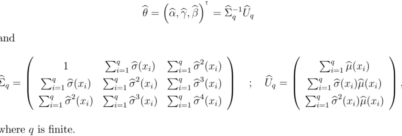
Theorem 2 Suppose that B2-B9 and D1-D3 hold. Let the marginal regressors Xs
satisfy Assumption C. Then the estimator (18) based on the sample observations
fYt; Xtgnt=1 satisfying either Assumption A1 or A2 is asymptotically normal with the
following limiting distribution:
r nh1+22p 1pexp 0h 2 2p 1 h b m(x) m(x) Bn(x) i =)N 0; 1 2(x) ; (33)
where Bn(x) = O(h ) is the ‘bias part’ in (28) and 2(x) = Var(YjX = x) is the
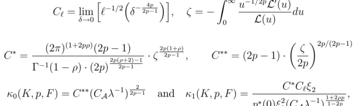
Below we explain the associated constants. Recall Assumption D1; under the condition, by the characterization theorem of Karamata (1933) (see e.g. Feller (1971)), there always exists a slowly varying function`(x)satisfyingF(1=x) =x `(x):Now …x somep, the order of increment constant for bandwidth in Assumption D3, and denote byL(t)the Laplace transform of X2. Then we have,
C` = lim !0 h ` 1=2 2p4p1 i ; = Z 1 0 u 1=2pL0(u) L(u) du C = (2 ) (1+2p )(2p 1) 1(1 ) (2p)2p( +2)2p 1 1 2p(1+ ) 2p 1 ; C = (2p 1) 2p 2p=(2p 1) 0(K; p; F) =C (CA 1) 2 2p 1 and 1(K; p; F) = C C` 2 p (0) 21(CA 1)1+21 2pp ; where ( )is the Gamma function, 1 and 2 are the constants speci…ed in (12) (which
simplify in case of uniform kernel for example), is the upper bound of the support of the kernel, and p ( )is the Radon-Nikodym derivative de…ned in D2. Recall that for the uniform (Box) kernel 2 = 21; so they cancel out in 2. See Dunker, Lifshits and
Linde (1998) and also Hong, Lifshits and Nazarov (2016) for some discussions on the underlying arguments for the formulation of these constants. To aid the exposition, we compute and present the constants for some common, regularly varying distributions in the table below.
Xj2 F i.i.d. limx!1`(x) = C` 2 Uniform(1,b) 1 1 n/a Gamma( ; ) 1 ( ) 1 1=2p sin( =2p) Exponential( ) 1 sin(1==22pp) Weibull( ; ) n/a Pareto( ; ) 1 = n/a 2 1 1=2 (2= )1=2 2 (1 2p)=2p sin( =2p)
Table 1: Examples of the key constants for some common distributions
For example, when Xj’s are Gaussian, the constants C and C denoted CG and
CG respectively, are given by:
CG= (2 ) (1 p)(2p 1) 2 (2p)32pp 11 2(1 2p)=2p sin( =2p) p 2p 1 ; CG = 2p 1 2 2psin2p ! 2p 2p 1 :
and 2(K; p; a) = CGC` 2 2 1 e 12k 1=2zk22(C A 1) p 1 2p 1
where z = (zj) = (j pxj) = D 1x. The exponential term in the denominator of the
asymptotic variance arises from the asymptotic equivalence relationship between the shifted and non-shifted small deviation for `2-valued Gaussian variables, cf. (31).
The CA constant represents the dependence structure across the marginal regres-sors and plays an important role. First of all, when the marginal regresregres-sors are identi-cally distributed and independent to each other, thenCA = 1. If not independent, the speci…c form of this constant is only known in the Gaussian case (by Hong, Lifshits and Nazarov (2016, Theorem 1.1). Speci…cally, when fXjgj is Gaussian and satis…es
Assumption C, given the square summable sequence aj in (30), we have
CA = " 1 2 Z 2 0 1 X j=0 ajexp(ijs) 1=p ds #p (34)
It is worth noting that interestingly, CA is a function of the spectral density of the MA(1) process fXjtgj.
The implications of the constantCA suggest an interesting …nding that allowing for dependence does not seem to incur much penalty; we conjecture that similar conclusion would hold for regressors of di¤erent distributions than Gaussian, but leave it for future studies.
4.3
Optimal Bandwidth
We now discuss the issue of bandwidth optimality. As in the …nite-dimensional frame-work, there is a bias-variance trade-o¤. As the bandwidth goes up, the variance gets smaller while the bias increases, and vice versa. Therefore we search for the optimal bandwidth hopt that balances the order of those two quantities.
We …rst suppose that p2 (c; ), cf. D3, is given:In the i.i.d. case with Gaussian regressor we have h s exp 0h 2=(2p 1) nh21pp1 ; (35) so that 2 + 1 p 2p 1 logh 0h 2 2p 1 logn:
Takingh (logn)a for somea <0 balances the leading terms on both sides:
2 + 1 p
2p 1 a log logn 0(logn) 2
2p 1a logn: (36)
The explicit ordera that solves (36) can be expressed in terms ofn, and p. Writing #:= [2 + (1 p)=(2p 1)] and := 2=(2p 1)for notational simplicity, and solving for a we have
aopt =
# W # 0 n =# logn
# log logn ; (37)
where W(y) is the Lambert W function (see e.g. Olver et al. (2010)), which returns the solutionxofy=x ex. From (37) the optimal bandwidthh
opt (logn)aoptfollows,
in which case the asymptotic root mean squared error is of the order(logn) aopt: Remark. We can look for the optimal bandwidth for the cases of non-Gaussian regressors by following exactly the same procedure as above; tedious details are omit-ted here. Regarding the solution in (37), since the mapping x 7! x ex is not an injection, the solution may be multi-valued on the negative domain, i.e. y < 0. This does not happen in (37) provided 1=4(however bigpis), because(1 p)=(2p 1)
is bounded away from 1=2; in this case, the coe¢ cient of the double logarithmic term in (36) is strictly smaller or equal to zero.
Since the log terms dominate the double logarithm in (36) as the sample size n increases, it can be readily expected that the optimal value of a in (37) converges to a limit in such a way that the leading orders are balanced. Below we introduce without formal justi…cation a trivial result that gives the lower bound (in…mum) of the optimal bandwidth (and hence of the optimal rate that balances the bias and variance). We remark that the result below holds for other choices of the distribution of the regressors, and also for the case of dependent (non-independent) regressors as allowed in Assumption C (i.e. when CA 6= 1), as the exponent of the leading term
2=(2p 1) remains invariant as is clear from Theorem 2. Nonetheless, it is worth noting that although the order of the convergence rate remains the same, the di¤erence in associated constants does make the speed at whichaopt converge to the limit in (38).
null
satis-fying Assumption D1, the order of the optimal bandwidth aopt satis…es
aopt #
2p 1
2 as n ! 1; (38)
which suggests that the lower bound of the optimal bandwidth is given by (logn) 2p21 h
opt (logn)aopt: (39)
This result tells us the best possible performance we can expect from the optimal bandwidth. Because nk(logn) (2p 1)=2
! 1 for any real k > 0, it follows that we cannot possibly estimate the regression function at a polynomial rate. This result is consistent with and complements the …ndings of Mas (2012, Theorem 3), which were obtained under the assumption of independence of regressors. The paper also considered the case where the bandwidth grows exponentially: j exp(jq)for some
q >0. Then for hj = jh, his result suggests exp[ (logn)2q=(2q+1)] hopt exp[aopt
(logn)bopt]. Therefore, the performance is better in general in this case, although obviously a polynomial rate of convergence still cannot be attained. It is not clear what will happen when the regressors are allowed to be dependent in the sense of Assumption C, since the behaviour of the small ball probability for non-independent (and non-Gaussian) sequence is not known for the case of exponentially decaying weights.
Returning back to Corollary 3, we emphasize that the arguments are true for any p 2 (c; ): Let pmax = supp2 (c; )p: Then a lower bound on the optimal bandwidth
(over allp) is(logn) (pmax 12): For example, whenc
j = (1=2)j 2 we have pmax= 1= :
Unfortunately, it is generally the case that pmax 2= (c; ); in which case the lower
bound is not quite achievable by our method.
Remark. Regarding bandwidth selection, one possibility is the Bayesian band-width selection methods like proposed in Zhang, King, and Hyndman (2006). We take as prior for h the density proportional to 1=(1 + h2) and as prior for p 1=2
the density of a 2(w)random variable. The hyperparameters ; w may be chosen by
experimentation. The priors are combined with a Gaussian (least squares) density to deliver a posterior for the bandwidth. The reader is referred to Section 5 for further discussions on the issue of bandwidth choice.
4.4
Uniform consistency
Uniform consistency of the Nadaraya-Watson estimator was …rst studied by Nadaraya (1964, 1970) and subsequently by numerous others. To mention few early papers, Devroye (1978) weakened the regularity conditions required in the previous papers, and Robinson (1983) proved uniform consistency for dependent sample data. In the functional statistics literature, uniform consistency of kernel estimators for conditional mean is established only with respect to i.i.d. sample data so far (see for example Ferraty et al. (2010), Ferraty et al. (2011), Kudraszow and Vieu (2013), and Kara-Zaïtri et al. (2017)) as far as the authors are concerned.
In this section, we show uniform consistency of our estimator under the (suitably modi…ed) regularity conditions assumed in the previous sections. We start by intro-ducing the notion of Kolmogorov’s entropy below. For some of its ealier discussions in statistics literature, the reader is referred to Yaracos (1985) and Mammen (1991). Definition 5. Given some >0, let L(S; )be the smallest number of open balls in
E of radius needed to cover the set S E. Then Kolmogorov’s -entropy is de…ned
as logL(S; ).
This quantity will be used in explaining the topological restrictions we adopt to suitably accommodate in…nite dimensionality. The de…nition implies the dependence of Kolmogorov’s entropy both on the nature of the space under study and the measure of proximity. It will be shown later in this section that the entropy is closely related to the rate of convergence of the estimator, in particular, to the penalty incurred on the rate in the uniform case. It is well known that the regression function cannot be estimated uniformly over the entire space, e.g. Bosq (1996). In our in…nite dimensional framework, the in…nite sequence spaces, if unrestricted, cannot be covered by a …nite number of balls, and that L(S; ) =1. We propose to consider uniform consistency over a subset ofR1, whose e¤ective dimension is truncated and is increasing in sample sizen. In particular, we de…ne the set
S := uj(ui)i2Z+; uj = 0 for all j > ;kuk1 R1; (40)
where = n is some increasing sequence and is …xed, and consider uniform
con-sistency over this compact set. Then Kolmogorov’s entropy of the set S is given as follows:
Lemma 2 Kolmogorov’s -entropy of S with = n(! 1) and >0 is logL S ; = log " 2 p + 1 ! # : (41) null
Remark. (41) is in line with common intuition; as the e¤ective dimension in-creases, the number of balls (with some …xed radius) required to cover the set tends to in…nity. Lemma 2 can be shown by exploiting the splitting technique and then by covering the polyhedron of increasing dimension. See appendix for details. Note that for …xed and = n, Kolmogorov’s entropylogL(S ; )is of order( log log ). Considering the de…nition of the setS , in the sequel (with a slight abuse of nota-tion) we takeX to denote the regressor, but with zeros after its th(=
n ! 1asn!
1)entry; that is, X = (X1; X2; : : : ; X ;0;0; : : :)
|
(so that the originalX is recovered as n ! 1). Also, the regression operator and the estimator with respect to this truncated regressor are denoted by m ( ) and mb ( ), respectively. All assumptions, including the additional one to follow below, are understood to hold under these mod-i…cations.
Assumption E
E. For su¢ ciently largen, Kolmogorov’s -entropy logL(S ; ) satis…es
(logn)8+2
n'x(h) logL(S ; )
p
n'x(h)
(logn)1+ for some 2(0;1=2): (42)
Furthermore,0< 'x(h) h <1 and (logn)2=(n'
x(h)) !0 as n! 1.
Remark. The …rst part of Assumption E speci…es the rate at which Kolmogorov’s en-tropy should behave with sample size n(hence in dimension = n). From the upper
and lower bound it readily follows thatn'(h)must be of order larger than(logn)6+2.
This assumption is su¢ ciently general. For example, in view of the bias-variance op-timal bandwidth suppose h (logn) (2p 1)=2 so that n'(h) (logn)(2p 1) . In this
case, assumption (42) is valid as long aspis moderately large enough relative to 1
in such a way that 6 + 2 (2p 1) . The second part is standard; in particular, the last condition straightforwardly follows by (42) and only slightly strengthens the bandwidth condition in Assumption B2.