Comparison of very high spatial resolution satellite image
segmentations
A. Carleer
a, O. Debeir
b, E. Wolff*
aa
Institut de Gestion de l'Environnement et d'Aménagement du Territoire, Université Libre de
Bruxelles, cp 130/02, Avenue Franklin Roosevelt, 50, 1050 Brussels, Belgium;
b
Information and Decision Systems, Université Libre de Bruxelles, cp 165/57, Avenue Franklin
Roosevelt, 50, 1050 Brussels, Belgium
ABSTRACT
Since 1999, very high spatial resolution data represent the surface of the earth with more details. However, information extraction by computer-assisted classification techniques proves to be very complex owing to the internal variability increase in land-cover units and to the weakness of spectral resolution 1, 2, 3. The increase in variability decreases the
statistical separability of land-cover classes in the spectral space 4. Per pixel multispectral classification techniques are
then insufficient for an extraction of complex categories and spectrally heterogeneous land-cover, like urban areas 5. Per
region classification was proposed as an alternative approach 6, 7. The first step of this approach is the segmentation. A
large variety of segmentation algorithms were developed these last 20 years 8 and a comparison of their implementation
on very high spatial resolution images is necessary. For this study, four algorithms from the two main groups of segmentation algorithms (boundary-based and region-based algorithms) were selected. In order to compare the algorithms, an evaluation of each algorithm was carried out with empirical discrepancy evaluation methods. This evaluation is carried out with a visual segmentation of IKONOS panchromatic images.
Keywords: segmentation, very high spatial resolution satellite images, evaluation methods. 1. INTRODUCTION
The first commercial very high resolution satellite (IKONOS) became accessible in autumn 1999 and the QuickBird satellite in October 2001. These new sources of very high resolution images are increasing the amount of information available on land cover at local to national scales 9. These data provide amazing details of the earth surface but
information extraction using computer-assisted classification techniques appears to be much more complex.
1.1 Internal variability
These new sources of very high resolution images don't provide necessarily better classification, this observation had already been made by Irons et al. (1985)4 at the time of the marketing of the Landsat-4 Thematic Mapper (TM) images.
The refinement of spatial resolution from 80 to 30 m did not often improve classification accuracy, even though the advantages of a higher resolution system appeared obvious when visual comparisons were made between TM and MSS imagery. This incongruous result of earlier studies had been attributed to one consequence of change of spatial resolution. With the spatial resolution refinement, the internal variability within homogenous land cover units increases
1, 2, 3, 6. The increased variability decreases the statistical separability of land cover classes in the spectral data space.
This decreased separability tends to depress per pixel classification accuracies, such as maximum-likelihood classification algorithms. The increased variability was attributed to the imaging of diverse class components by higher resolution sensors, whereas at coarser resolutions, sensors integrated the reflected spectral radiance of the various components, and classes appeared more homogeneous 4.
1.2 Spectral resolution
An other disadvantage with the very high spatial resolution satellite images, is the relatively poor spectral resolution. While the spatial resolution is fine, spectral capabilities are limited compared to sensors like Landsat TM. Generally, there is a trade-off between the spatial resolution and the spectral resolution 2, 10. The spectral sensibility of the receptor
cell requires a sufficient instantaneous field of view (IFOV). The spectral resolution depends on the ratio of signal to noise, and this ratio is linked to the IFOV, the height of flight and the opto-electronic characteristics of receptor cell 11. *[email protected]; phone +32 2 650 50 76; fax +32 2 650 43 24; http://www.ulb.ac.be/igeat
Image and Signal Processing for Remote Sensing IX, edited by Lorenzo Bruzzone, Proceedings of SPIE Vol. 5238 (SPIE, Bellingham, WA, 2004) · 0277-786X/04/$15 · doi: 10.1117/12.511027 532
1.3 Region based procedure
To overcome these problems, a region based procedure can be used. The segmentation procedure is successful at removing much of the structural clutter, and performs well in comparison with traditional majority filtering 5. This
alternative approach had been proposed by Hill in 1999 7 to reduce local spectral variation. Image regions are more
homogeneous in themselves than with nearby regions and represent discrete objects or areas in the image. Segmented images are useful in following purposes:
− segmented images can be easier to interpret 12;
− the classification of these segmented images is often more accurate than per pixel classification, overcoming the
misclassification problem due to the internal variability of the regions 9.
1.4 Spatial information
Spatial information is used in order to increase the classification accuracy for spectrally heterogeneous classes 11 and to
overcome the current spectral limitations of very high spatial resolution satellite images 13. The spatial information can
be carried out from segmented images; spatial attributes being calculated for each region. The attributes can be the surface, the perimeter, the compactness (area/perimeter²), the degree and kind of texture 14. In the per pixel methods, the
spatial attributes are calculated on an arbitrary neighborhood using mobile windows. The image segmentation enables us to obtain the specific spatial attributes of the regions, without taking into account nearby regions. Moreover, the spatial attributes, like texture, calculated with mobile windows, create between-class texture, which is often more distinctive than within-class texture. This between-class texture causes an edge effect in the classification 15. This edge
effect problem could disappear with segmentation.
2. OBJECTIVE
A large variety of segmentation algorithms were developed these last 20 years 8 and a comparison between them on
very high spatial resolution satellite images is necessary. This paper presents an evaluation and comparison study of different types of segmentation algorithms on very high spatial resolution satellite images.
3. SEGMENTATION ALGORITHMS
Segmentation algorithms can conveniently be classified as boundary-based and region-based 8, 16, 17, 18. Boundary based
algorithms detect object contours explicitly by using the discontinuity property and region based algorithms locate object areas explicitly according to the similarity property 8. The boundary approach gathers the contours detection
techniques. These methods do not lead directly to a segmentation of the image because obtained contours are seldom related, so it is necessary to carry out closing contours if one wishes a complete segmentation of the image. Indeed, after contours closing, the duality contours/regions appears clearly. A region is defined as the inside of a closed line. On the other hand, the methods of the region approach lead directly to a segmentation of the image, each pixel being affected with a single region 19. For this study, algorithms from each group have been selected.
3.1 Boundary-based algorithms
Two algorithms of this group have been selected: "Optimal edge detector" 19 and "Watershed segmentation" 20.
In "Optimal edge detector", the procedure first filters the image with the Canny-Deriche filter. This filter provides the derivative of the images and takes into account the Canny criterion: namely 'good' detection (low probability of missing real edges and detecting noise), 'good' position estimation and single response to each edge, which also accomodates edges of a finite width. Next, a hysteresis thresholding 21, 22 is achieved on the image to preserve the coherent
boundaries. Finally, contours are closed by the way of best count. The count is calculated by the sum of the pixels norm constituting the way in the gradient image.
In the "Watershed segmentation" 20, the procedure first transforms the original data into a gradient image. The
resulting grey tone image is considered as a topographic surface. We flood this surface from its minima and we prevent the merging of the waters coming from different sources, thus we partition the image into a set of watershed lines. The catchment's basins should correspond to the homogeneous regions of the image. Before transforming the original data into a gradient image, we can apply a median filter on the image to reduce the noise. The presence of noise in an image causes an over-detection of contours by the morphological gradient. The median filter locally homogenizes the image and avoids extrema gradients and thus parasitic contours. It is also a good means not to take into account object texture
during contours detection. The image gradient can also be thresholded to limit the contour sensitivity. E.g., if the threshold is 10, we keep pixels with a gradient higher than 10 and the others are put at 0 as if there are no edges.
3.2 Region-based algorithms
In this group, two algorithms have been selected: "Multilevel thresholding technique" 23 and "Region-Merging"
technique.
"Multilevel thresholding" algorithm is a global thresholding of grey tone image which uses second-order grey level statistics. The segmentation is carried out from non symmetric co-occurrence matrix. For all grey levels, the conditional estimated probabilities of intensity transition between two regions separated by the grey level n are calculated. The
lower the value of this estimated probability, the lower the probability that the next transition will be in a different intensity class. Therefore, it is assumed that meaningful sets of thresholds would correspond to the minima of this measure. Then, the minima are searched on a range of a number neighbour grey levels on both sides of the grey level n.
These minima are used as image segmentation thresholds 23, 24.
In the "Region-Merging" technique, the procedure starts at each point in the image with one-pixel objects and in
numerous subsequent steps, smaller image objects are merged into bigger ones, throughout a pair-wise clustering process. The underlying optimization procedure minimizes the weighted heterogeneity nh of resulting image objects,
where n is the size of a segment and h an specific definition of the heterogeneity. If the smallest growth exceeds the
threshold defined by the user, the process stops. The definition of heterogeneity mixes a criterion for spectral heterogeneity with a criterion for spatial heterogeneity, in order to reduce the deviation from a compact or smooth shape 25, 26, 27. This procedure was developed by DEFIENS Imaging in its eCognition software.
4. TEST IMAGES
The test images are VHR satellite images of various types of landscape. They are extracted from an IKONOS panchromatic image of June 8, 2000, on the Brussels-Capital Region area in Belgium (Fig. 1). The extent of the extracts is 256 m by 256 m and the spatial resolution is 1m. The various landscape types are rural (RURAL), residential (RESI), urban administrative zone (ADM), urban dwelling zone (DW) and forest (FOREST) (Fig. 1). Each extract is visually segmented. The visual segmentations are used as reference for the assessment. A visual segmentation method was defined, on the basis of visual interpretation, in order to homogenize the various extract segmentations. The visual segmentation method consists in three main points:
− we selected an appropriate minimum size of four pixels, for the smallest region to be represented 28;
− we placed the boundaries of adjacent region at the center of the transition zone between them but if the transition
zone occurs consistently, it is considered to be a separated object 29;
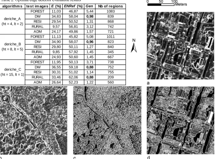
Figure 1: IKONOS image extension of June 8, 2000 and the image extracts: a) Administrative zone (ADM), b) Dwelling zone (DW), c) Rural zone (RURAL), d) Residential zone (RESI) and e) Forest zone (FOREST).
5. EVALUATION METHODS
Segmentation algorithms can be evaluated analytically or empirically 30. The analytical methods directly examine and
assess the segmentation algorithms themselves by analyzing their principles and properties. The empirical methods indirectly judge the segmentation algorithms by applying them to test images and measuring the quality of segmentation results compared with reference segmentations (empirical discrepancy methods) or by measuring some desirable properties of segmented images (empirical goodness methods). For this study, we have chosen empirical discrepancy evaluation methods. Indeed, analytical methods are easier to apply, but they often only provide qualitative
test im ages local variance FOREST 10,46 DW 14,92 RESI 13,21 RURAL 6,21 ADM 12,82
Table 1: Mean local variance of images.
properties of algorithms. Empirical methods are normally quantitative, as the values of quality measures can be numerically calculated. Among them, goodness methods based on subjective measures of image quality are adapted for an objective evaluation of segmentation algorithms. Discrepancy methods can be both objective and quantitative 30.
The first selected method is the discrepancy based on the number of mis-segmented pixels in the segmented images compared with the visually segmented reference images 30.
Considering the segmentation as a pixel classification process, the percentage of mis-classified pixel is a measurement of discrepancy. Suppose an image made up of Nref pixel classes, a confusion matrix C of dimension Nref can be
constructed, where each entry Cij represents the pixel number of class j classified as class i by the segmentation algorithms. The discrepancy measure is defined as:
, 100 1 1 1 1 1 × − =
∑∑
∑
∑∑
= = = = = ref ref ref ref ref N i N j ij N k kk N i N j ij C C C Ewhere the numerator represents the number of pixels mis-classified and the denominator is the total number of pixels in the test image.
In this evaluation method, the same importance isn't given to small and great regions. A segmentation with great regions could give a small percentage of classified pixels whereas the majority of the small regions are mis-segmented. We should give the same importance to small and great regions. Therefore, we modify the first discrepancy measure. This new measure is based on the same principle as the first method but the percentage of mis-classified pixels is calculated on each reference region and after that the mean percentage is calculated. The new discrepancy measure is defined as:
, 100 1 1 ref N i iref N j ij N N n C E ref ref ref
∑
=∑
= × =where niref is the number of pixels in the region i (class i) of the reference segmentation image.
The second evaluation method selected is a simple ratio between the number of regions in the segmented image and thz number of regions in the reference segmentation. This ratio is the Generalization and is defined as:
, ref s N N Gen=
where Ns is the number of regions in the segmented image and Nref is the number of regions in the reference
segmentation. This measure allows to evaluate the over-segmentation (Gen > 1) or the under-segmentation (Gen < 1) of
tested algorithms 20. Over-segmentation is not a defect in itself because it could be recovered during the classification of
the regions, but if the over-segmentation is significant, the advantages of carrying out an image segmentation before classification are lost. Usually, with the increase in number of regions, errors are expected to decrease 24. However,
under-segmentation cannot be recovered during classification because the objects are mis-identified 20.
The most important evaluation measure is the average error by region (ENRef) which makes it possible to give the same
weight to all the regions of the visual segmentation. It is all the same interesting to analyze the total error (E), for a high total error value, being the consequences of either small or great regions, is not desirable. The Gen evaluation measure is not the most important measure in the segmentation methods evaluation
except if we note an under-segmentation. It enables us to know if the advantage of carrying out a segmentation is not lost. To complete and to help the interpretation of the evaluation, we have also calculated the mean local variance (Table 1) and the gradient image of each extract (test images). The mean local variance is calculated within a 3x3 pixels variance filter. The mean local variance provides a measure of internal variability of the extracts 1.
6. RESULTS
First, the results of algorithm evaluations are presented separately (6.1 to 6.4) after which they will be compared (6.5).
6.1 Optimal edge detector (Canny-Deriche optimal filter)
Three sets of high- (ht) and low-thresholds (lt) are selected for the hysteresis thresholding (ht = 4 and lt = 2, ht = 8 and lt = 5, ht = 15 and lt = 1). The results are presented in Table 2. The over-segmentation values (Gen) are reasonable and
even go as far as under-segmentation with the DW image test, which is an important defect of the segmentation. The under-segmentation of DW and RURAL (deriche-C) test images and the very low over-segmentation of ADM, RESI and RURAL (deriche-B) test images are due to a low identification of object contours. Part of the object contours were removed after the optimal filtering in these test images. This bad contour detection is confirmed by high total errors (E)
and high average errors by region (ENRef).
Figure 2: a) Gradient image of the ADM test image, b) Gradient image of the FOREST test image, c) deriche_A FOREST test image segmentation and d) deriche_A ADM test image segmentation.
The change of hysteresis thresholding thresholds doesn't change anything about the errors and over-segmentation for the ADM, RESI and DW test images. Part of the objects in these three images are enough contrasted and homogeneous, and thus the object borders are characterized by strong gradients which are always detected with a high high-threshold. A low high-threshold doesn't detect more borders because the objects are more homogeneous (less local maxima within those). The fact that the RURAL and FOREST test images are more textured than the others explains that over-segmentation decreases as the threshold increases. With a low high-threshold, the result of the over-segmentation is parasitized by the local maxima resulting from the object texture. With a high high-threshold, the borders due to the
algorithm s test im ages E (%) ENRef (%) Gen Nb of regions
FOREST 11,03 46,87 5,44 1083 DW 34,83 58,04 0,98 839 RESI 29,54 50,52 1,31 868 RURAL 9,57 56,81 3,12 742 ADM 24,17 49,86 1,57 721 FOREST 11,13 45,82 5,08 1011 DW 34,90 58,07 0,96 823 RESI 29,80 50,11 1,27 840 RURAL 9,85 57,92 1,45 345 ADM 24,93 50,60 1,45 667 FOREST 11,95 50,13 3,71 738 DW 36,55 59,18 0,88 752 RESI 30,31 51,02 1,14 755 RURAL 33,46 62,06 0,88 209 ADM 26,64 52,23 1,22 560 deriche_A (ht = 4, lt = 2) deriche_B (ht = 8, lt = 5) deriche_C (ht = 15, lt = 1)
texture disappear but the object borders which are less contrasted can also disappear as it is the case with the RURAL test image. With the RURAL image the total error (E) strongly increases with the high-threshold going from 8 up to 15.
The ascending order of the absolute number of regions resulting from the segmentation gives us a curious order (Table 2): FOREST > RESI > DW > RURAL > ADM. This order doesn't follow the ascending order of the mean local variance (Table 1) as one could expect. This could be explained by the distribution of the maxima within the gradient images (Fig. 2). The fact that the FOREST image test is more segmented while not having the greatest mean local variance, can be explained by the objects within this image being comparedly textured and little contrasted; this leads to the detection of many local maxima in the gradient image and thus detection of many contours of many regions. On the other hand, for the ADM test image for which the mean local variance is high, the number of regions resulting from the segmentation is lower. The objects in this image are contrasted and more homogeneous (less textured); this explains the greater mean local variance and a fewer number of regions. Indeed, the local maxima of gradient image correspond to the objects borders and not to their texture. As appeared in other studies 1, 6 ,a high mean local variance doesn't
necessarily indicate the presence of strongly textured objects. An image of homogenous contrasted objects, can provide an higher mean local variance than an image of textured non-contrasted objects, as is the case with the ADM and FOREST images (Fig. 2).
The segmentations of the RURAL and FOREST test images give a total error (E) below 15% but have an average error
by region (ENref) over 45% which is not acceptable in a segmentation. One notices that the average errors by region are
significant for all test images. This is explained by the fact that an image does not only consist of homogeneous and contrasted objects or textured and little contrasted objects, but of a proportion of both; for this reason the choice of suitable thresholds is difficult. If the high-threshold is high, many contours will be missing. It is not profitable to take it too low, because in this case, the result can be parasitized: by having a lower high-threshold, some pixels not corresponding to desired contours are preserved and are then unfortunately supplemented by connexity in complete contours in the final result.
This contour detection method is adapted for homogeneous and contrasted objects detection like buildings but not for whole image segmentation.
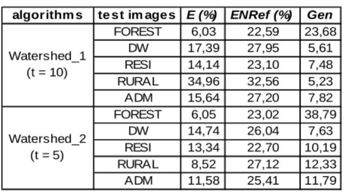
6.2 Watershed segmentation
As forthe contour detection method by Canny-Deriche operator (optimal filtering), the test images are filtered. In this method the filter is a median filter of 3x3 pixels instead of the Canny-Deriche optimal filter. Median filtering makes it possible to remove the noise while preserving contours. Moreover, the gradient images are thresholded by a simple threshold and the contour detection is carried out by watershed. Two simple thresholds are selected for this segmentation (10 and 5).
It is noticed that the change of threshold doesn't change the total errors (E) and average errors by region (ENref) for the
ADM, DW, RESI and FOREST test images, there is a light decrease in these two errors. On the other hand, the change of threshold has a great influence on the total error of the RURAL test image for which the total error (E) falls from 35% to 8%. That is explained by the detection of new contours delimiting objects of the visual segmentation which were not detected previously. One also notes a big increase of the over-segmentation for FOREST test image with a reduction of the threshold. The reduction of the threshold allows the identification of maxima not corresponding to contours in the gradient image: the segmentation is parasitized. One can say about the FOREST test image that identifiable contours by this method had already been detected with a threshold of 10 since there is no improvement of the total error and average error by region. Broadly, the use of a threshold of 5 works well on all test images; the best results were obtained with this threshold. Similar results were already obtained with a threshold of 10 except for RURAL test image where contours were missing.
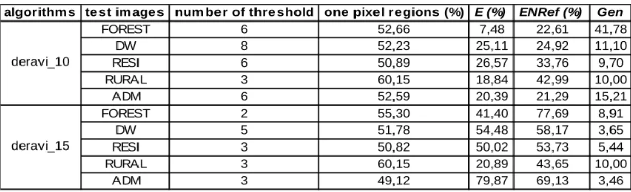
6.3 Multilevel thresholding technique (Deravi and Pal segmentation)
Two numbers of neighbouring grey levels (10, 15) are selected for the search of the minima, the evaluation results are in Table 4. In the multilevel thresholding segmentation, there is a significant salt and pepper effect which contributes to the over-segmentation of images. Because of the high local variance, the adjacent pixels aren't in the same range of grey
algorithm s te st im ages E (%) ENRef (%) Gen
FOREST 6,03 22,59 23,68 DW 17,39 27,95 5,61 RESI 14,14 23,10 7,48 RURAL 34,96 32,56 5,23 ADM 15,64 27,20 7,82 FOREST 6,05 23,02 38,79 DW 14,74 26,04 7,63 RESI 13,34 22,70 10,19 RURAL 8,52 27,12 12,33 ADM 11,58 25,41 11,79 Watershed_1 (t = 10) Watershed_2 (t = 5)
values between two thresholds, which explain the salt and pepper effect. Between 49 and 60 percent of the regions are made of one pixel. A modal filter could have been passed after the thresholding, but that would not improve the errors because the one pixel regions are contained in a reference region and are consequently well segmented.
The total errors (E) are above 20% (deravi_10) except for FOREST but then the over-segmentation is very significant. The thresholding methods are less effective on images presenting a unimodal histogram. Such histograms are typical in images with many small different objects such as aerial photographs or very high spatial resolution satellite images. The histogram of the image RURAL (Fig. 3) test is bimodal but the two peaks don't represent contrasted objects and background. These images don't exhibit a clear background-foreground distinction 23 (Fig. 3).
Figure 3: a) RURAL test image, b) deravi_10 RURAL test image segmentation, c) Histogram of the RURAL test image.
This method could be used to isolate particular objects in an image, e.g. objects having a particular spectral characteristic (peak in the histogram), but not to segment an image whatever the landscape. The method is appropriate for images of objects on an homogeneous background or for images of homogeneous, adjacent and contrasted objects, as it is the case for the ADM test image which present the smallest average error by region (Deravi_10). However a problem remains with the images of contrasted objects, like urban images: if the number of thresholds is sufficient, the transition zone between contrasted objects will be isolated as an object. The value of the transition zone falls in an other range of value as the two adjacent objects. This effect disappears if the number of thresholds decreases (from deravi_10 to deravi_15) but the errors are too significant.
Finally, it should be mentioned that the method is applicable when the scene is of object-background nature 31 and the
texture level is not very high.
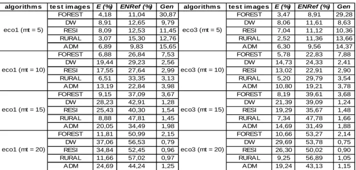
6.4 Region-Merging technique
In this region-merging technique, the main merger criterion is the region variance (spectral heterogeneity), the other merger criterion is a region form criterion (spatial heterogeneity). A different weight can be given to each one of these criteria in the merger value calculation which cannot exceed an a priori fixed merger threshold. Four merger-thresholds
Table 4: Multilevel thresholding technique evaluation results
algorithm s test im ages num ber of threshold one pixel regions (%) E (%) ENRef (%) Gen
FOREST 6 52,66 7,48 22,61 41,78 DW 8 52,23 25,11 24,92 11,10 RESI 6 50,89 26,57 33,76 9,70 RURAL 3 60,15 18,84 42,99 10,00 ADM 6 52,59 20,39 21,29 15,21 FOREST 2 55,30 41,40 77,69 8,91 DW 5 51,78 54,48 58,17 3,65 RESI 3 50,82 50,02 53,73 5,44 RURAL 3 60,15 20,89 43,65 10,00 ADM 3 49,12 79,87 69,13 3,46 deravi_10 deravi_15
(mt = 5, 10, 15, 20) ac well as two weights were selected for both criterions and led to eight different segmentations. The eco1 algorithm doesn't take into account the region form criterion whereas the eco3 does. The results are presented in Table 5.
One notices that the best results are obtained by taking the form into account (eco3), all merger thresholds taken together and for all test images. The results are obviously the best with the smallest merger threshold (5). With a small merger threshold, mergers of pixels and regions are limited and there is a considerable over-segmentation, which results into decreasing errors.
While the merger threshold goes from 5 up to 10, the total errors (E) for eco3 and for all landscapes remain lower than 15% and increase in a limited way for RURAL and FOREST test images. The average errors by region (ENRef) for
"eco3 mt = 10" are included between 20 and 30 % and there is a very significant decrease of the over-segmentation. In this method, it can be noticed that all test images respond in the same way to the change of parameters. We also observe that with small merger threshold and with contrasted objects, the transition zone (more or less one pixel wide) between objects is isolated as an object as with the Multilevel thresholding technique. The merger threshold isn't high enough for
the transition zone to be included in one of the two objects. When the merger threshold increases from 10 to 15, this transition zone disappears but the errors are too big.
When the merger threshold increases up to 20, the over-segmentation (Gen) decreases as far as under-segmentation for some images. The total error remains lower than 10% for FOREST and RURAL test images but the average error by region (ENref) reaches 57% which is unacceptable.
6.5 Comparison
For similar high-thresholds, the contour detection by "watershed" is more effective than by the Canny-Deriche operator from the point of view of the total error and average error by region. On the other hand, watershed segments a little more than Canny-Deriche operator, which could partly explain these best results. The median filter retains more contours than the Canny-Deriche optimal filter.
The "Watershed segmentation" with a threshold of 5 is equivalent to the "region-merging" segmentation with a merger threshold of 10 but over-segmentations are higher for the Watershed segmentation. The results would be better with a smaller threshold but over-segmentation would be high as is the case with a decrease of the merger threshold in the region merging technique.
The "multilevel thresholding" technique is effective for images having a histogram including peaks and valleys, which is seldom the case for very high spatial resolution satellite images. And if the segmentation is good it is to the detriment of a reasonable over-segmentation value. The "region-merging" method works well with textured images
algorithm s te st im ages E (%) ENRef (%) Gen algorithm s test im ages E (%) ENRef (%) Gen
FOREST 4,18 11,04 30,87 FOREST 3,47 8,91 29,28 DW 8,91 12,65 9,79 DW 8,06 11,61 8,63 RESI 8,09 12,53 11,45 RESI 7,04 11,12 10,36 RURAL 3,07 15,30 12,76 RURAL 2,52 11,36 13,66 ADM 6,89 9,83 15,65 ADM 6,30 9,56 14,37 FOREST 6,88 26,84 7,53 FOREST 5,78 22,83 7,88 DW 19,44 29,23 2,56 DW 14,73 24,33 2,41 RESI 17,55 27,64 2,99 RESI 13,02 22,91 2,90 RURAL 6,51 33,35 3,13 RURAL 5,20 29,79 3,54 ADM 13,19 22,84 3,98 ADM 10,80 19,21 3,78 FOREST 9,15 37,09 3,67 FOREST 8,19 39,61 3,68 DW 28,23 42,91 1,28 DW 21,39 39,09 1,24 RESI 25,43 40,30 1,54 RESI 19,29 35,67 1,48 RURAL 8,88 47,81 1,45 RURAL 7,34 47,78 1,66 ADM 20,05 34,49 1,98 ADM 14,69 31,49 1,88 FOREST 11,81 50,99 2,15 FOREST 10,66 53,27 2,14 DW 37,06 56,53 0,79 DW 29,69 53,78 0,75 RESI 34,84 52,45 0,96 RESI 26,30 50,02 0,90 RURAL 11,66 57,02 0,97 RURAL 9,25 56,89 1,05 ADM 24,69 44,24 1,25 ADM 19,24 43,13 1,15 eco3 (mt = 5) eco3 (mt = 10) eco3 (mt = 15) eco3 (mt = 20) eco1 (mt = 5) eco1 (mt = 10) eco1 (mt = 15) eco1 (mt = 20)
and images of not very contrasted objects like in RURAL and FOREST test images. The results obtained with the other types of landscapes are not bad. It is perhaps the method which gives a good image segmentation of any type of landscape without having high over-segmentation values and this method does not require pre- and post-processing like filters or contours closing. Moreover, there isn't any salt and pepper effect as with "multilevel thresholding" segmentation. These two segmentation methods are in the same group of methods (region-based algorithms) but the segmentation procedures are very different. The "multilevel thresholding" segmentation uses the global information of the image to segment it (the detection of thresholds is influenced by all pixels in the image) when the "region-merging" segmentation uses the local information (region variance and form) to segment the image. The global information methods are more sensitive to texture (internal variability), i.e., less immune to texture than the local information based methods 31.
7. CONCLUSION
The miraculous segmentation method which segments in a correct way for all types of landscape does not exist. In each of the four used methods, the choice of the parameters (thresholds) is important and has a great influence on the segmentation results.
The contour detection methods are sensitive to noise or texture in the images and a pre-processing is essential in the majority of the cases (median filter, optimal filter...). These methods prove to be effective for the detection of homogeneous and contrasted objects within the images as in the images of urban zones where these types of objects are very common (buildings...).
The two region-based methods are very different and a common conclusion isn't obvious. However, a problem with the transition zones between the contrasted objects can be present in both segmentation techniques. The "region-merging" segmentation is less sensitive to texture, which is a significant advantage in the segmentation of very high spatial resolution satellite images.
All the objects in an image cannot be isolated with one segmentation without over-segmentation. If each region of the segmentation to represent one object in the image, multi-level segmentation must be applied. In each level different objects are isolated according to their characteristics (texture, form...). The lower levels are made up of small objects, larger homogenous objects and pieces of the larger textured objects. The upper levels are made up of the merger of the regions of the lower levels and allow the identification of larger textured objects. The implementation of multi-level segmentation is easier with the region-merging technique, as long as the merger threshold is increased.
ACKNOWLEDGMENTS
IKONOS images were acquired by the I.G.E.A.T. (Institut de Gestion de l'Environnement et d'Aménagement du Territoire, Université Libre de Bruxelles) within the framework of a feasibility study funded by the OSTC (federal Office of the Scientific, Technical and Cultural affairs) within the framework of TELSAT 4 program. The authors give special thanks to the GdR ISIS of the CNRS (Groupe de Recherche en "Information-Signal-Image-Vision" du Centre National de Recherche Scientifique français) for the access to the SIMPA (Signal and IMages softwares PAckages) software library. Alexandre Carleer would like to thank the FRIA (Fonds pour la Formation à la Recherche dans l'Industrie et l'Agriculture) for its support.
REFERENCES
1. J.L. Cushnie, The interactive affect of spatial resolution and degree of internal variability within land-cover types on classification accuracies, International Journal of Remote Sensing, 8 (1), 15-29, 1987.
2. P. Alpin, P.M. Atkinson, P.J. Curran, Fine spatial resolution satellite sensors for the next decade, International Journal of Remote Sensing, 18 (18), 3873-3881, 1997.
3. Y. Zhang, Texture-Integrated classification of urban treed areas in high-resolution color-infrared imagery,
Photogrammetric Engineering and Remote Sensing, 67 (12), 1359-1365, 2001.
4. J.R. Irons, B.L. Markham, R.F. Nelson, D.L. Toll, D.L. Williams, R.S. Latty, M.L. Stauffer, The effects of spatial resolution on the classification of Thematic Mapper data, International Journal of Remote Sensing, 6 (8),
1385-1403, 1985.
5. S. Barr, M. Barnsley, Reducing structural clutter in land cover classification of high spatial resolution remotely-sensed images for urban land use mapping, Computers and Geosciences, 26, 433-449, 2000.
6. C.E. Woodcock, A.H. Strahler, The factor of scale in remote sensing, Remote Sensing of Environment, 21,
7. R.A. Hill, Image segmentation for humid tropical forest classification in Landsat TM data, International Journal of Remote Sensing, 20 (5), 1039-1044, 1999.
8. Y.J. Zhang, Evaluation and comparison of different segmentation algorithms, Pattern Recognition Letters, 18,
963-974, 1997.
9. P. Alpin, P.M. Atkinson, P.J. Curran, Fine spatial resolution simulated satellite sensor imagery for land cover mapping in the United Kingdom, Remote Sensing of Environment, 68, 206-216, 1999.
10. T. Key, T.A. Warner, J.B. McGraw, M.A. Fajvan, A comparison of multispectral and multitemporal information in high spatial resolution imagery for classification of individual tree species in a temperate hardwood forest ,Remote Sensing of Environment, 75, 100-112, 2001.
11. T.M. Lillesand and R.W. Kiefer, Remote Sensing and Image Interpretation, pp. 750, John Wiley & Sons, Inc., New York, 1994.
12. S. Ryherd, C. Woodcock, Combining spectral and textural data in the segmentation of remotely sensed images,
Photogrammetric Engineering and Remote Sensing, 62 (2), 181-194, 1996.
13. B. Guindon, Combining diverse spectral, spatial and contextual attributes in segment-based image classification,
ASPRS Annual Conference, Washington DC, May 22-26, 2000.
14. K. Johnsson, Segment-based land-use classification from SPOT satellite data, Photogrammetric Engineering and Remote Sensing, 60 (1), 47-53, 1994.
15. C.J.S. Ferro, T.A. Warner, Scale and texture in digital image classification, Photogrammetric Engineering and Remote Sensing, 68 (1), 51-63, 2002.
16. B. Nicolin, R. Gabler, A knowledge-based system for the analysis of aerial images, IEEE Transactions on Geoscience and Remote Sensing, 25 (3), 317-329, 1987.
17. L.L.F. Janssen, M. Molenaar, Terrain objects, their dynamics and their monitoring by the integration of GIS and remote sensing, IEEE Transactions on Geoscience and Remote Sensing, 33 (3), 749-758, 1995.
18. B. Guindon, Computer-based aerial image understanding: A review and assessment of its application to planimetric information extraction from very high resolution satellite images, Canadian Journal of Remote Sensing, 23 (1),
1997.
19. J.P. Cocquerez, S Philipp, Analyse d'images: filtrage et segmentation, pp. 457, Masson, Paris, 1995.
20. O. Debeir, Segmentation supervisée d'images, Ph.D., Faculté des Sciences Appliquées, Université Libre de Bruxelles, 2001.
21. Z. Hou, T.S. Koh, Robust edge detection, Pattern Recognition, 36 (9), 2083-2091, 2003.
22. L. Ding, A. Goshtasby, On the Canny edge detector, Pattern Recognition, 34, 721-725, 2001.
23. F. Deravi, S.K. Pal, Grey level thresholding using second-order statistics, Pattern Recognition Letters, 1, 417-422,
1983.
24. S. Biswas, N.R. Pal, On hierarchical segmentation for image compression, Pattern Recognition Letters, 21,
131-144, 2000.
25. eCognition user guide, Definiens Imaging, München, Germany, 2003.
26. C. Burnett, T. Blaschke, A multi-scale segmentation/object relationship modelling methodology for landscape analysis, Ecological Modelling, Article in Press, 2003.
27. C.J. van der Sande, S.M. de Jong, A.P.J. de Roo, A segmentation and classification approach of IKONOS-2 imagery for land cover mapping to assist flood risk and flood damage assessment, International Journal of Applied Earth Observation and Geoinformation, 4, 217-229, 2003.
28. R. Welch, Spatial resolution requirements for urban studies, International Journal of Remote Sensing, 3 (2),
139-146, 1982.
29. J.B. Campbell, Introduction to Remote Sensing, pp. 622, Taylor & Francis, London, 1996.
30. Y.J. Zhang, A survey on evaluation methods for image segmentation, Pattern Recognition, 29 (8), 1335-1346,
1996.