Classifier Fusion For Multimodal Correlated Classifiers And Video Annotation

ISTANBUL TECHNICAL UNIVERSITY_FGRADUATE SCHOOL OF SCIENCE ENGINEERING AND TECHNOLOGY

CLASSIFIER FUSION FOR

MULTIMODAL CORRELATED CLASSIFIERS AND VIDEO ANNOTATION

M.Sc. THESIS Ümit EKMEKÇ˙I

Department of Computer Engineering Computer Engineering Programme

ISTANBUL TECHNICAL UNIVERSITY_FGRADUATE SCHOOL OF SCIENCE ENGINEERING AND TECHNOLOGY

CLASSIFIER FUSION FOR

MULTIMODAL CORRELATED CLASSIFIERS AND VIDEO ANNOTATION

M.Sc. THESIS Ümit EKMEKÇ˙I

(504101540)

Department of Computer Engineering Computer Engineering Programme

Thesis Advisor: Assoc. Prof. Dr. Zehra ÇATALTEPE

˙ISTANBUL TEKN˙IK ÜN˙IVERS˙ITES˙IFFEN B˙IL˙IMLER˙I ENST˙ITÜSÜ

BA ˘GIMLI SINIFLANDIRICILAR VE V˙IDEO ˙I ¸SARETLEME ˙IÇ˙IN SINIFLANDIRICI B˙IRLE ¸ST˙IRME

YÜKSEK L˙ISANS TEZ˙I Ümit EKMEKÇ˙I

(504101540)

˙

Bilgisayar Mühendisli˘gi Anabilim Dalı Bilgisayar Mühendisli˘gi Programı

Tez Danı¸smanı: Assoc. Prof. Dr. Zehra ÇATALTEPE

Ümit EKMEKÇ˙I, a M.Sc. student of ITU Graduate School of Science Engineering and Technology 504101540 successfully defended the thesis entitled“CLASSIFIER FUSION FOR MULTIMODAL CORRELATED CLASSIFIERS AND VIDEO ANNOTATION”, which he/she prepared after fulfilling the requirements specified in the associated legislations, before the jury whose signatures are below.

Thesis Advisor : Assoc. Prof. Dr. Zehra ÇATALTEPE ... Istanbul Technical University

Jury Members : Assoc. Prof. Dr. Hazım Kemal EKENEL ... Istanbul Technical University

Dr. Aydın ULA ¸S ... Argela A. ¸S.

...

Date of Submission : 5 May 2014 Date of Defense : 27 May 2014

To my family,

FOREWORD

I would like to thank Dr. Zehra ÇATALTEPE for her guidance and support during my graduate studies. I would also like thank to my family for their endless support and love.

May 2014 Ümit EKMEKÇ˙I

TABLE OF CONTENTS Page FOREWORD... ix TABLE OF CONTENTS... xi ABBREVIATIONS ... xiii LIST OF TABLES ... xv

LIST OF FIGURES ...xvii

SUMMARY ... xix ÖZET ... xxi 1. INTRODUCTION ... 1 1.1 Eigenclassifiers ... 2 1.2 REPERE challenge ... 2 1.3 Contributions ... 3

2. BACKGROUND and NOTATION ... 5

2.1 Notation ... 5

2.2 Background... 5

2.2.1 Principal Component Analysis ... 5

2.2.2 Kernel Principal Component Analysis ... 6

3. RELATED WORK ... 9

4. EXTENDED MULTIMODAL EIGENCLASSIFIERS and CRITERIA FOR FUSION MODEL SELECTION ... 13

4.1 Introduction ... 13

4.1.1 Variance-Bias Trade off ... 14

4.2 Eigenclassifiers ... 15

4.3 Extended Eigenclassifiers with Multimodal Base Classifier Outputs ... 17

4.3.1 Unimodal Case ... 17

4.3.2 Recoding of inputs... 18

4.3.3 Multimodal Case ... 19

4.4 Fusion Method Experiments... 20

4.4.1 Simple Average... 21

4.4.2 Kernelized Extended Multimodal Eigenclassifiers... 21

4.4.3 SVMs and Eigen SVMs... 21

4.4.4 Dropout... 21

4.4.5 AYSU dataset... 23

4.4.6 Fusion Experiment Results... 24

4.5 Criteria for Fusion Method Selection ... 27

4.5.1 Average Eigenvalue Distributions and Diversity Metrics... 27

4.6 Conclusion ... 30

5. FUSION FOR VIDEO ANNOTATION ... 33

5.1 REPERE Dataset ... 33

5.2 General Information on Speaker Identification Task... 33

5.3 Propagation Based Fusion for Unsupervised Speaker Identification Task... 34

5.4 Supervised Speaker Identification Task... 35

5.4.1 Extracting candidate names from diarization and written names... 35

5.4.2 Propagation over similarity graph ... 35

5.4.3 Overall Algorithm ... 36

5.4.4 Results and Discussion ... 36

6. CONCLUSIONS ... 39 REFERENCES... 41 APPENDICES ... 45 APPENDIX A ... 47 CURRICULUM VITAE ... 49 xii

ABBREVIATIONS

AdaBoost :Adaptive Boosting Bagging :Bootstrap Aggregating EC :Eigenclassifiers

EGER :Estimated Global Error Rate KEC :Kernelized Eigenclassifiers

KXMEC :Kernelized Extended Multimodal Eigenclassifiers MKL :Multiple Kernel Learning

PCA :Principal Component Analysis SVM :Support Vector Machines

XMEC :Extended Multimodal Eigenclassifiers

LIST OF TABLES

Page

Table 4.1 : Test accuracies of fusion methods on AYSU dataset collection ... 25

Table 4.2 : Number of experiments each method performed the best... 25

Table 4.3 : Average rank of each ensemble method... 26

Table 4.4 : Average eigenvalue distribution ... 29

Table 4.5 : Average divergence metrics... 29

Table 5.1 : EGER results on test and development datasets for Supervised Method ... 37

Table 5.2 : EGER results on test and development datasets for Unsupervised Method ... 37

Table A.1 : Detailed information on AYSU [1] datasets... 47

LIST OF FIGURES

Page Figure 4.1 : The ensemble methods shown in red are significantly different

than the ensemble method shown in blue according to Tukey’s critical value range shown by the vertical blue line. ... 26 Figure 4.2 : Variance of estimators for Eigenclassifiers (red) and Extended

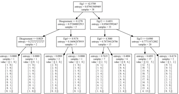
Multimodal Eigenclassifiers (blue). ... 26 Figure 4.3 : Basic rules found by Decision Tree... 30

CLASSIFIER FUSION FOR

MULTIMODAL CORRELATED CLASSIFIERS AND VIDEO ANNOTATION

SUMMARY

Classifier fusion has become one of the key challenges in machine learning due to the increase in size and structural richness of available data. Thanks to the advances in computing power, we are also able to train many different classifiers; instead of using a single one of them we try to combine them hoping to get better performance. Classifier fusion benefits from classifiers as accurate and as independent as possible. How to generate independent local or base classifiers is a critical question. Adaboost Algorithm of Freund and Schapire (1994) and Bagging Algorithm of Breiman and Leo (1996) aim to create independent base classifiers by using different subsets of inputs generated through sampling for each classifier. Another method, which is used in this thesis, is the Eigenclassifiers approach, proposed by Alpaydın and Ulas in 2012. Eigenclassifiers method aims to create uncorrelated base classifier outputs by mapping to an uncorrelated space. However, for multiclass classification problems, since there are redundant features in the Eigenclassifier transformed classifier output space, they have correlations between them and this causes higher estimator variance and lower prediction accuracy. In this thesis, we extend Eigenclassifiers method to obtain truly uncorrelated base classifiers. We also generalize the distribution on base classifier outputs from unimodal to multimodal, which lets us handle the class imbalance problem.

There are many different classifier fusion methods, and the question of which one to use for a given dataset needs to be answered. In this thesis, we try to answer this question also. We generate a dataset by calculating the performances of nine different fusion methods on 38 different datasets provided by Ulas et. al in 2009. We investigate accuracy-diversity relationship of ensembles on this experimental dataset by using eigenvalue distributions and diversity metrics given by Kuncheva and Whitaker in 2001. We obtain basic rules which can be used to decide on a fusion method given a dataset.

In the second part of the thesis we use classifier fusion for video annotation. We develop a supervised method to combine audio and text information. The proposed method increases the accuracy by about 13 percent over the unimodal methods. This part of the thesis was done as part of a collaborative European Union project called Camomile that brings together researchers from four countries and six institutions together.

BA ˘GIMLI SINIFLANDIRICILAR VE V˙IDEO ˙I ¸SARETLEME ˙IÇ˙IN SINIFLANDIRICI B˙IRLE ¸ST˙IRME

ÖZET

˙Internet kullanıcılarının sayısının artması, sosyal ileti¸sim platformu kullanıcılarının artmasına ve böylece her geçen gün internet üzerinde var olan bilgi boyutunun armasına sebep olmaktadır. Ayrıca sosyal platformlardaki yapısal zenginli˘gin artması, örne˘gin Facebook’un insanlar arasındaki ili¸skileri arkada¸slık ba˘glantıları sayesinde grafiksel düzeyde, payla¸sılan yazılar ve yorumlar sayesinde yazımsal düzeyde ve payla¸sılan resimler ve olu¸sturulan galeriler sayesinde görsel düzeyde ara¸stırmacılara sunması, bu farklı yapıdaki bilgilerin birle¸stirilebilmesi problemini oldukça önemli bir konu haline getirmektedir. Bu tür veri kümeleri sayesinde, bir sınıflandırma problemini çözmek için de˘gi¸sik veri örnekleri, öznitelik türleri ve sınıflandırma yöntemleri kullanılarak e˘gitilmi¸s çok sayıda sınıflandırıcı elde edilebilmektedir. Sınıflandırıcı birle¸stirme yöntemleri, eldeki sınıflandırıcıları birle¸stirerek daha iyi ba¸sarıma ula¸smayı hedeflemektedir.

Sınıflandırıcıların birle¸stirilmesi geç birle¸stirme (late fusion) ya da erken birle¸stirme (early fusion) yöntemleri ile yapılabilir. Daha sık kullanılan geç birle¸stirme yönteminde birden fazla yerel sınıflandırıcı çıkı¸sı ba¸ska bir sınıflandırıcının e˘gitilmesi ile birle¸stirilir. Geç birle¸stirme yönteminin ba¸sarılı olması için gerekli olan önemli bir unsur yerel sınıflandırıcı çıkı¸slarının birbirlerinden mümkün oldu˘gunca ilintisiz olmasıdır. Çünkü yerel sınıflandırıcıların ilintisiz olması birle¸stirme için kullanılan sınıflandırıcının varyansının azalmasına, dolayısı ile de ba¸sarımının artmasına sebep olmaktadır. Yerel sınıflandırıcılar arasındaki ilintisizlik farklı yollardan elde edilebilir. Örne˘gin aynı hata fonksiyonunu azaltmayı hedefleyen sınıflandırıcılar farklı giri¸sler üzerinde e˘gitilebilirler. Boosting ve Bagging algoritmaları bu yöntemin en bilinen örneklerindendirler. Bunun haricinde aynı giri¸sler üzerinde farklı amaç fonksiyonuna sahip sınıflandırıcılar ya da farklı mimariye, parametrelere sahip (örne˘gin farklı sayıda saklı sinir hücresine sahip yapay sinir a˘gları gibi) sınıflandırıcılar e˘gitilerek de sınıflandırıcılar arasında ilintisizlik olu¸sturulabilir.

Alpaydın ve Ula¸s tarafından 2012 yılında önerilen, aynı zamanda bu tezin ilk kısmının temelini olu¸sturan, Eigenclassifiers (Özsınıflandırıcılar) yöntemi yerel sınıflandırıcı çıkı¸sları arasındaki ilintisizli˘gi do˘grusal bir dönü¸süm olan Temel Bile¸senler Analizi (PCA: Principal Component Analysis) dönü¸sümünü kullanarak gerçekle¸stirmeyi amaçlamaktadır. Fakat bu dönü¸süm kullanılırken çoklu etikete sahip problemlerde, etiketler arasındaki ili¸skiler ele alınmadı˘gı için dönü¸süm sonucu olu¸san özellik yöneyleri tam olarak do˘grusal ilintisiz olmamaktadır. Bu durum özellik yöneylerinde fazladan ve gereksiz verinin olu¸smasına ve varyansın artmasına, dolayısı ile performansın dü¸smesine sebep olmaktadır. Bu tez çalı¸smasının ilk kısmında Eigenclassifiers yöntemi çok sınıflı sınıflandırma problemleri için geni¸sletilerek dönü¸süm sonucu elde edilen özellik uzayı do˘grusal olarak tam ilintisiz hale

getirilmi¸stir. Bu sayede, sınıflandırıcı çıkı¸slarını birle¸stiren sınıflandırıcı varyansı dü¸sürülerek performans artırılmı¸stır.

Çok sınıflı sınıflandırma problemlerinde e˘ger bir sınıfta gözlemlenen örnek sayısı di˘ger sınıflardakilerden çok fazla ise, hata fonksiyonunu azaltmayı hedefleyen sınıflandırıcılar bütün örnekleri o sınıfa atayabilmektedir. Bu dengesiz örnek-etiket da˘gılımı problemi Eigenclassifiers yönteminin yerel sınıflandırıcı çıkı¸slarının çok modlu Gauss da˘gılımı izledi˘gi varsayılarak tezde çözümlenmi¸stir.

Verilen bir veri kümesi için hangi sınıflandırıcı birle¸stirme yönteminin daha uygun oldu˘gu önemli bir sorudur. Bu soruya cevap bulabilmek için, tezde, dokuz farklı sınıflandırıcı birle¸stirme yönteminin, 38 farklı veri kümesi üzerindeki performansları hesaplanarak, deneyimsel bir veri kümesi olu¸sturulmu¸stur. Sınıflandırıcı birle¸stirme yöntemleri olarak Ortalama, Eigenclassifiers, Extended Multimodal Eigenclassfiers, Dropout, Support Vector Machines (do˘grusal ve do˘grusal olmayan çekirdekli), Eigen Support Vector Machines, Kernelized Eigenclassifiers ve Kernelized Extended Multimodal Eigenclassifiers kullanılmı¸stır. Olu¸sturulan veri kümesi üzerinde Dropout yönteminin en iyi performansı verdi˘gi görülmü¸stür. Geni¸sletilmi¸s Eigenclassifiers yöntemi Eigenclassifiers yöntemine göre daha iyi performans göstermi¸s, çekirdek-le¸stirilmi¸s yöntemler ise Dropout’tan sonra en iyi sonuçları vermi¸stir. Olu¸sturulan veri kümesi üzerinde sınıflandırıcı birle¸stirme yöntemlerinin do˘gruluk-ilintisizlikleri, 2001 yılında Kuncheva ve Whitaker tarafından önerilen sınıflandırıcı ilintililik ölçütleri (Q statistics, correlation coefficient ρ, disagreement measure, double-fault measure ve

entropy) kullanılarak kar¸sıla¸stırılmı¸stır. Ayrıca, tezde bilindi˘gi kadarı ile ilk olarak, ortalama özde˘gerler da˘gılımı kullanılarak da do˘gruluk-ilintisizlik yorumu yapılmı¸stır. Bir karar a˘gacı yardımı ile hangi sınıflandırıcı birle¸stirme yönteminin uygun oldu˘guna dair kurallar çıkarılmı¸stır. Elde edilen ilk sonuçlara göre Destek Vektör Makineleri tabanlı sınıflandırıcı birle¸stirme yöntemleri do˘grusal ilintisi az olan veri kümeleri üzerinde ön plana çıkarken test edilen di˘ger sınıflandırıcı birle¸stirme yöntemleri do˘grusal ilintisi daha fazla olan veri kümeleri üzerinde ön plana çıkmaktadır. Karar a˘gacı tarafından çıkarılan kurallara göre en önemli ayırt edici özelliklerin elde edilen özde˘gerler ve disagreement measure oldu˘gu görülmektedir.

Tezin ikinci kısmında, video i¸saretleme (video annotation) için sınıflandırıcı birle¸stirme yöntemleri kullanılmı¸stır. Bu kısımda bir Chistera projesi olan,

Collaborative Annotation of multi-modal, multi-lingual and multi-media documents, CAMOMILE kapsamında çalı¸smalar yapılmı¸stır. CAMOMILE projesi üzerinde dört ülkeden altı ara¸stırma grubu çalı¸smaktadır. Projenin amacı televizyon programlarında kimlerin konu¸stu˘gunu ya da kimlerin gözüktü˘günü, farklı bilgi kaynaklarını birle¸stirerek bulmaktır. Projedeki ba¸slıca bilgi kaynakları görüntü, ses ve altyazılardır. Projede kullanılan REPERE veri kümesi iki farklı Fransız kanalından, BFM TV, LCP, yedi farklı televizyon programından 30 saat kayıt edilmi¸s 188 videodan olu¸smaktadır. Bu veri kümesi 24 saati e˘gitim, üç saati geli¸stirme ve üç saati test olmak üzere üç parçaya ayrılmı¸stır. Tezde, ses bilgisi ve altyazı bilgisi birle¸stirilerek hem gözetimsiz (unsupervised) hem de gözetimli (supervised) olarak o anda kimin konu¸stu˘gu bulunmaya çalı¸sılmı¸stır. Ses bilgisi olarak, Camomile proje katılımcısı Claude Barras’ın (LIMSI) ekibi tarafından geli¸stirilen ve projedeki ara¸stırmacılara sunulan konu¸smacıların kümelenmi¸s fakat etiketlenmemi¸s (speaker diarization) halleri kullanılmı¸stır. Altyazı bilgisi olarak ise proje katılımcısı Georges Quénot (LIG-CNRS) tarafından elde edilen, televizyon

programlarının ekranın alt kısmında gösterdikleri, konu¸smacıların isimlerini içeren yazıların i¸slenmesi ile elde edilen konu¸smacıların isimleri kullanılmı¸stır. Böylelikle, video i¸saretlemede ses ve yazı kullanılarak sınıflandırıcı birle¸stirmede, elde edilen bölütlenmi¸s fakat etiketlenmemi¸s konu¸smacı kümeleri ve konu¸smacılara ait etiketlerin çıkarıldı˘gı altyazı bilgisi bulunmaktadır. Yöntemler geli¸stirilirken, özellikle, önceki çalı¸smalarda ba¸sarı göstermi¸s olan yayılım ve grafik e¸sle¸stirme tabanlı algoritmalar üzerinde durulmu¸stur. Gözetimsiz olarak Bredin tarafından önerilen term-frequency, inverse document-frequency (TF-IDF) tabanlı yayılım algoritması kullanılmı¸stır. Gözetimli yöntemler tasarlanırken konu¸smacı tanıma üzerine çıkı¸s üreten 3 farklı sınıflandırıcının çıkı¸sları kullanılmı¸stır. Bu çıkı¸slar özellikle yayılım tabanlı benzerlik grafi˘gi olu¸sturulurken, dü˘gümler arasındaki benzerli˘gin hesaplanması a¸samasında kullanılmı¸stır. Özellikle yanlı¸s tahmin edilen örneklerin sayısını azaltarak katkı sa˘glayan bir di˘ger yöntem ise kendi aralarında aynı konu hakkında konu¸san ki¸silerin bir araya gruplanması ve bu grupların zaman aralıklarına denk gelen altyazılardan isimlerinin çıkartılarak, gruplar için aday isim listelerinin çıkarılmasıdır. Tezde 2014 yılında yayımlanan REPERE test kümesi üzerinde sonuçlar hesaplanmı¸stır. Elde edilen sonuçlara göre farklı bilgi kaynaklarının birle¸stirilmesi tek bilgi kayna˘gı kullanımına göre performansta %13 lük bir artı¸s sa˘glamı¸stır. Bunun yanında tezde elde edilen sonuçlar projenin Fransız ortakları tarafından elde edilen sonuçlarla da kar¸sıla¸stırılmı¸stır.

1. INTRODUCTION

Every year not only the size of the data, but also the heterogeneous structure of the data gets richer. For example social networks bring graphical representation of the interactions between both people and their behaviors. Also Twitter, Foursquare and other social networks give a lot of textual information to the researchers that was not available before. For a bioinformatic problem protein-protein interactions a researcher can both have a graphical representation of interactions, protein sequences and a gene ontology annotations [2]. Combining these different representations can give huge benefits to the researchers. For video annotation problems our source of information can be the face images, the audio of the people, the subtitles of the speech [3] and the colors of the clothes [4] that people wear. Using these different sources of information to identify a person will clearly increase the robustness and the accuracy. Another kind of problem that fusion helps is the case where there is just one representation of the data but there can be more than one model defined to explain the generative process. In the best case, each model handles one independent property of the process. For example, for a city the monthly temperature change can show different properties over the months. In summer the temperature can increase linearly and smoothly and in spring the temperature change can follow a periodic signal. To model this behavior of the data we can linearly combine the models that we generated. Fusion is generally performed in two levels: early fusion or late fusion. In the early fusion, features extracted from the different sources of the data are first combined and then sent to a classifier. In the late fusion, first each decision of the independent models are obtained and then using a final classifier, local decisions are combined. The advantage of the early level fusion is the capability to handle the correlation between multiple features from different modalities at an early stage. Also, it requires only one learning phase on the combined feature vector. Advantage of late fusion over the early fusion is that it allows to use the most suitable model for each modality and if local decisions are treated as probabilities they will be on the same scale which requires more work to have the same effect on the early fusion.

This thesis consists of two parts. In the first part we deal with the problems, which have one representation and multiple base classifiers. In practice base classifiers are correlated which affects the performance of fusion negatively. Eigenclassifiers [5] is one of the methods that try to decorrelate the base classifiers before combining them with a linear classifier. In the first part we showed how to kernelize the Eigenclassifiers, how to reduce the variance of the final stage estimator and hence improve the prediction accuracy and how to extend the distribution on the data to mixture of Gasussians to handle the imbalance data problem more accurately than Eigenclassifiers. In the second part we deal with a problem which has multiple representations and one classifier. We especially focused on the REPERE challenge and tried to identify people in TV broadcast shows by combining text and speech information.

In the following sections we briefly describe Eigenclassifiers [5] and the REPERE challenge. In section 1.3 the contributions of the thesis are given.

1.1 Eigenclassifiers

Eigenclassifiers were proposed by Ulas, Yıldız and Alpaydın in 2012. In practice most of the base classifiers are correlated with each other. One approach is to keep a small subset of base classifiers by reducing the correlated pairs, but if there are correlations between base classifiers, then it is clear that this will cause loss of information. Eigenclassifiers combine base classifiers taking into account that they are not independent. They treat the outputs of base classifiers as a feature vector and find a new uncorrelated feature space which is then combined with a stack classifier. In their work, Ulas, Yıldız and Alpaydın compared their method with AdaBoost [6] and Bagging [7]. They observed that Eigenclassifiers are either more accurate or achieve a comparable accuracy using a fewer number of classifiers.

1.2 REPERE challenge

The REPERE challenge aims to support the development of automatic systems for multimodal person identification. Dataset contains 30 hours of videos taken from two French TV channels with multimodal annotations, i.e speech transcriptions, extracted names from subtitles, video annotations. The dataset mostly contains news and debates. Dataset is divided into three parts, train (24h), development (3h) and test

(3h). There are two main tasks in the challenge, who is speaking and when?, who is seen and when?. Our contributions and results on 2014 test dataset are given in Chapter 5.

1.3 Contributions

Eigenclassifiers method [5] aims to reduce the correlation between base classifiers by a linear projection of base classifier outputs to a new uncorrelated feature space. As we will see in Chapter 4, Eigenclassifiers method does not use the correlations between class assignments. This causes redundant features to be produced when the test data is mapped using the transformation matrix computed on the training set. In this thesis, in order to avoid redundant features, we adopt the Eigenclassifiers method to use correlation between class assignments and to obtain truly uncorrelated base classifiers. We also relax the unimodal distribution assumption on base classifier outputs in order to handle the class imbalance problem. There are other well known fusion methods and the question of which fusion method should be used for a particular dataset is an important one. In order to answer this question, we generate an experimental database by calculating the results of nine different fusion methods on 38 different datasets used in AYSU dataset [1]. We experiment with the following fusion methods: simple Average, Eigenclassifiers [5], Extended Multimodal Eigenclassifiers, Dropout [8], Support Vector Machines (with linear and RBF kernels), Eigen Support Vector Machines, Kernelized Eigenclassifiers and Kernelized Extended Multimodal Eigenclassifiers. On the experimental dataset, we investigate the relationship between accuracy and diversity of an ensemble to decide on the suitable classifier fusion method for a particular case. We obtain basic rules that show which fusion method works best on a particular dataset. In the second part of the thesis propagation based unsupervised and supervised methods we used in the REPERE challenge are explained. Especially the two proposed methods we focus on, reducing the candidate labels for each diarization and propagation based similarity graph, help to improve performance by decreasing the number of false-positives. We present both our results and our French partners’ results on the REPERE test dataset released in 2014.

The rest of the thesis is organized as follows. In Chapter 2, we introduce the notation we use and give some background on the base methods we use. Related work is given

in Chapter 3. Extended Multimodal Eigenclassifiers with strategy for fusion method selection is introduced in Chapter 4. In Chapter 5, multimodal fusion algorithms for video annotation are explained. Conclusions and future work are provided in the last Chapter.

2. BACKGROUND and NOTATION

In this chapter, we first introduce the notation used in the thesis. We also go through the Principal Component Analysis (PCA) and Kernel PCA which is used at the kernelization process of Eigenclassifiers [5]

2.1 Notation

In order to describe our task in more concrete mathematical terms, we introduce the following notation. Vectors are denoted by lower case and bold characters, ex: x, Matrices are denoted by upper case and bold characters, ex: X and scalar values are denoted by lower case characters. When we are given a classification problem with

K classes, N instances andRtrained base classifiers we denote the the base classifier outputs for instancei,i=1...N, byR×Kdimensional matrixXi∈RR×K. Each entry

inXi,xr_i,k∈[0 : 1]is the probability value given by classifier rfor thekth label. Φ(x)

is a non-linear mapping from some low dimensional space to an higher dimensional space and is induced by the decided kernel functionK . kxk2_{denotes the vector norm} of x and is the same as the dot product <x,x>. kXkF denotes matrix norm and

can be calculated bytrace(XTX). The eigenvalues of a positive definite matrixX are denoted byλ1≥λ2≥. . .≥λnand the corresponding eigenvectors are denoted by v1,v2, . . . ,vn. 1ndenotes the vector whose all values are 1 and1n×ndenotes the matrix

whose all elements are 1.In×ndenotes the identity matrix of sizen×n.

2.2 Background

2.2.1 Principal Component Analysis

PCA (principal component analysis) is at the heart of the eigenclassifiers, since we will need its formulation for kernelized eigenclassifiers also, we briefly explain PCA below. PCA is an unsupervised dimensionality reduction method. It is a linear mapping that maps the original space to a new space which covers as much of the variance in the data

as possible and giving an uncorrolated direction for each added dimension. We explain PCA from this view of maximum variance formulation. If we assume that we have a set of observations{xn}wheren=1, . . . ,N, then our goal is to project the data onto

a space where the variance of the projected data is maximum and the dimensionality is less or equal than the original data. If we defineW as a projection matrix then the projected data isY =WT(X−X). The variance of the projected dataE[Y YT]is given by:

WTE[(X−X)(X−X)T]W =WTSW (2.1) whereSis the data covariance matrix ofXandXis a matrix that consists of the mean vector of the data at each row.

To maximize projected variance WTSW with respect to W and the constraint WTW =I (we are only interested in a direction) we introduce a diagonal Lagrange multiplier matrixΛ. Then the objective function to maximize is:

WTSW+Λ(I−WTW) (2.2)

The derivative of this function with respect toW is:

SW =WΛ (2.3)

This is a familiar equation where the columns of the W is the eigenvectors ofS and digonal elements of Λare the eigenvalues of S. When we multiply both sides of 2.3

withWT and we get the projected variance asWTSW =Λ. SinceWTW =I, in

order to maximize the variance we should select the eigenvectors which corresponds to largest eigenvalues.

2.2.2 Kernel Principal Component Analysis

For kernel PCA, instead of the original inputsxnwe study withφ(xn)which are the

basis function values. 1 LetΦbe then×mmatrix of basis function values for the n

observed items, soΦik=φk(xi). Even ifX have zero mean probablyΦwill not have

zero mean. We should centralize the basis matrix as:

Φ= [In×n−1n×n/n]Φ (2.4)

1_{For kernel PCA formulation, we follow the notation used in Radford M. Neal’s lecture notes in} http://www.utstat.utoronto.ca/ radford/sta414.S12/week12.pdf.

whereIn×n is then×nidentity matrix and1n×nis the matrix whose all elements are

1. We can now find eigenvectors of

ΦΦT = [In×n−1n×n/n]ΦΦT[In×n−1n×n/n] (2.5)

Now if we substitute a kernelK(x,x)instead ofΦΦT then we get a centralized kernel matrix

K = [In×n−1n×n/n]K[In×n−1n×n/n] (2.6)

letv1, v2,. . ., vnbe the eigenvectors andλ1≥λ2≥. . .≥λnbe the eigenvalues, then

the projection of a data pointx∗on them’th principal component is

[k−1T_nK/n][In×n−1n×n/n]vm/ p

λm (2.7)

where k is the vector of dimension n with k_i=K(x_∗,x_i) and 1T_n is a raw vector all ones.

3. RELATED WORK

Simple average and weighted average combination are the most well known and frequently used methods for classifier combination. Fumera and Roli [9] in 2005 investigated the theoretical and experimental analysis of these linear combiners. In the case of the weighted average they considered the simplest and the most widely used implementation of weighted average, where a set of nonnegative weights are assigned to each individual classifier. The conclusion they reached was, only for small classifier ensembles, if the individual classifiers exhibit a range of errors with non-negligible width (at least 0.05) and if the outputs of the individual classifiers are highly correlated, then weighted average can perform better than single average with the condition that a suitable validation data are available for optimal weight estimation [9]. The effect of correlation and variance of base classifiers in biometric authentication task is studied by PoH and Bengio [10] in 2005. One of the most important findings was, while positive correlation hurts fusion, greater diversity improves fusion. The other well known methods are minimum, maximum, median and majority voting. Kuncheva [11] performed a theoretical study on these fusion strategies. Minimum/maximum rule was found to be the best for uniformly distributed classifier outputs and for normally distributed outputs the methods gave very similar results. The work assumed the independence of the estimates which is restrictive and unrealistic for most cases. There are ensemble methods that try to overcome this restriction by trying to reduce the dependency among classifiers. ADAboost [6] and Bagging [7] are the two of the well known ones and the Eigenclassifiers [5] method is the one proposed by Ulas, Yıldız and Alpaydın. Performance comparison of Eigenclassifiers with ADAboost and Bagging is given in [5]. There are probabilistic classifier combination methods too. In the simplest case classifier outputs are assumed to be conditionally independent given the true class labels. Ghahramani and Kim [12] proposed three methods to model the correlation between classifier outputs. The first one was to define a hidden variable representing the difficulty of each data point and marginalizing over that variable resulting in a weakly dependent model. The second one was to explicitly

model the pairwise dependencies among classifiers using a Markov Network and the third one was the unification of the two models. They compared their methods with the independent case. SVM based fusion methods are mostly studied in the area of multimedia applications. For example Zhu, Yeh and Cheng [13] offered a fusion framework to classify the images, that have embedded text within their spatial coordinates, by combining visual and textual features with a pair-wise SVM.

The methods we mentioned above are all in the category of late fusion. The other level of fusion is the early fusion where the information is fused at the feature level. Multiple kernel learning (MKL) is one of the successful implementations of early fusion, especially because different information sources such as graphs or texts can be transformed into a common information representation, a kernel, and can be combined by that way. In 2006 Girolami and Zhong [14] adopted gaussian process priors and gave a fully bayesian solution to the problem of optimal combination of covariance functions (kernel functions). Because their model was fully probabilistic, from a bayesian view, inferring the weights of each kernel was nothing but the problem of inferring any unknown parameter. In 2012 Gonen [15] proposed a formulization that is fully conjugate bayesian model and derived a deterministic variational approximation which allowed them to combine hundreds or thousands of kernels very efficiently.

Especially for video annotation and identity detection in TV broadcasts, fusion of different modalities (speech, text and image) holds an important place in the literature. Poignant et. al. [3] proposed a method for unsupervised speaker identification in TV broadcast videos. Their first method was propagation of overlaid names (obtained via OCR) to the speech turns using a variant of the term frequency inverse document frequency (TF-IDF) information retrieval coefficient. Also Poignant et. al. [16] compared the pronounced names modality and written names modality and they concluded that despite a larger number of pronounced names ,speech to text errors and speech transcription errors reduce the potential of this modelity for naming speakers. Bredin et. al. [17] proposed a graph based fusion framework for person identification problem using diarization, written names information. For each video a multimodal probability graph is built and each vertices are connected by an edge weighted by the probability that they correspond to the same person. Person identification is achieved by looking for the maximum probability path between every turn and all available

identities. In 2012, Tapaswi, Bauml and Stiefelhagen [4] searched on identfying charaters in TV series. They aimed at labeling every character appearance, and not only where a face can be detected. They integrated face recognition, clothing appearance, speaker recognition and contextual constraints in a probabilistic manner. For the Big bang Theory dataset they achieved an improvement of 20% for person identification and 12% for face recognition.

4. EXTENDED MULTIMODAL EIGENCLASSIFIERS and CRITERIA FOR FUSION MODEL SELECTION

Diversity among base classifiers is one of the key issues in classifier combination. Although the Eigenclassifiers method proposed by (Ula¸s, Yıldız and Alpaydın, 2012), aim to create uncorrelated base classifier outputs, having redundant features in the transformed classifier output space causes higher estimator variance and lower prediction accuracy. In this thesis, we extend Eigenclassifiers method to obtain truly uncorrelated base classifiers. We also generalize the distribution on base classifier outputs from unimodal to multimodal, which lets us handle the class imbalance problem. We also aim to answer the question of which classifier fusion method should be used for a given dataset. In order to answer this question, we generate a dataset by calculating the performances of nine different fusion methods on 38 different datasets. We investigate accuracy-divergence relationship of ensembles on this experimental dataset by using eigenvalue distributions and divergence metrics defined by (Kuncheva and Whitaker, 2001). We obtain basic rules which can be used to decide on a fusion method given a dataset.

4.1 Introduction

Classifier combination allows fusion of different classifiers trained on different modalities, for example visual and audio based classifiers can be combined for better annotation of a video. Even when there is no obvious multimodality, using different features, instance subsets, different types of classifiers or objective functions, we may be able to obtain a set of classifiers whose combination outperforms the best single classifier. Although, in theory, to reduce the variance of the ensemble combination method as much as possible, the combined classifiers should be as diverse as possible [18], in practice, diversity and accuracy of classifiers are competing criteria.

Eigenclassifiers method [5] is one of the proposed methods that aim to reduce the correlation between base classifiers by a linear projection of base classifier outputs to

a new uncorrelated feature space. As we will see in the next section, Eigenclassifiers method does not use the correlations between class assignments. This causes redundant features to be produced when the test data are mapped using the transformation matrix computed on the training set. In this thesis, in order to avoid redundant features, we adopt the Eigenclassifiers method to use correlation between class assignments and to obtain truly uncorrelated base classifiers. We also relax the unimodal distribution assumption on base classifier outputs in order to handle the class imbalance problem. There are other well known fusion methods and the question of which fusion method should be used for a particular dataset is an important one. In order to answer this question, we generate an experimental database by calculating the results of nine different fusion methods on 38 different datasets used in AYSU dataset [1]. We experiment with the following fusion methods: simple Average, Eigenclassifiers [5], Extended Multimodal Eigenclassifiers, Dropout [8], Support Vector Machines (with linear and RBF kernels), Eigen Support Vector Machines, Kernelized Eigenclassifiers and Kernelized Extended Multimodal Eigenclassifiers. The methods Kernelized Eigenclassifiers and Eigen Support Vector Machines are introduced in [19] and to the best of our knowledge, Extended Multimodal Eigenclassifiers and kernelized version are introduced for the first time in this study. On the experimental dataset, we investigate the relationship between accuracy and diversity of an ensemble to decide on the suitable classifier fusion method for a particular case. We obtain basic rules that show which fusion method works best on a particular dataset.

The rest of the thesis is organized as follows. We introduce the notation used in the thesis, and show the relationship between the variance of an estimator and the prediction error in Section 4.1.1. In Section 4.2 and 4.3, we review Eigenclassifiers method of [5] and introduce our method of Extended Multimodal Eigenclassifiers. In Section 4.4, we give the results of 10 different fusion methods on 38 datasets. In Section 4.5, we introduce eigenvalue distributions and also use the diversity metrics defined by [20] to investigate accuracy-diversity relationship of ensembles on the experimental database we generate in Section 4.3. We obtain basic rules that can be used to select a suitable fusion method. Conclusions are given in Section 4.6.

4.1.1 Variance-Bias Trade off

Both Eigenclassifiers method and our Extended Multimodal Eigenclassifiers, use a linear combination of uncorrelated base classifier outputs for classification. Assuming

θ is the target value that we try to predict, the expected sum of squares loss can be

written as: E_d h (wTd−θ)2 i . (4.1)

The expected loss can be decomposed into bias and variance components as:

Eh(wTd−wTE[d] +wTE[d]−θ)2 i (4.2) =Eh(wTd−wTE[d])2i | {z } Var +E[(wTE[d]−θ | {z } Bias2 )2] =var(wTd) +Bias2 =wTCov(d)w+Bias2 (4.3)

Minimization of (4.3) can be achieved by diagonalizing Cov(d) and making wTw as small as possible, which corresponds to L₂ regularizer. Eigenclassifiers and our Extended Multimodal Eigenclassifiers use this information to create uncorrelated featuresd=UTXvwhose covariance is a diagonal matrix. The difference between the two methods is the way they treat the vectorv. Eigenclassifiers use the vectorv_gt which is previously known from the label information, on the other hand, Extended Multimodal Eigenclassifiers treatvas a vector to be optimized.

4.2 Eigenclassifiers

The key idea of Eigenclassifiers [5] is to create uncorrelated base classifiers that may help to reduce the prediction error by reducing the variance of the estimator. We first express this method using our notation.

Given the transformation matrix U and matrix X which is formed by the outputs of Rclassifiers for K classes for an instance, we first compute UTX ∈_RR×K_{. This}

matrix is flattened by concatenation of its column vectors to form a vector of dimension

R·K. For multimodal classification forK classes, instead of the weight vector w in Equation 4.3, we need to use a matrix W ∈_RR·K×K _{to get a linear combination of}

mapped classifier outputs. Let the operator Diag_U(UTM U), if possible, find the transformation matrixU which transforms matrixM to a diagonal matrix.

We can express the problem of computation of the transformation matrixU as:

Diag

U

(WTCov(d)W), (4.4)

whered=UTXvgt.

The purpose ofvgt is to select the column ofXwhich corresponds to the ground truth

label. We define the matrixXgt as:

Xgt= [X1vgt...Xivgt...XNvgt] (4.5)

which is the concatenation of columns that correspond to true labels. Let xgt =

Xvgt be the column gt of X. Using the definition of Cov(d) =E[ddT] and its

approximation by the training set, E[XvgtvgtTXT] = N1∑ N i=1x gt i x gtT i = 1 NXgtX T gt.

Substituting this expected value anddin Equation (4.4), we get:

Diag U (WTUTE[XvgtvTgtXT]U W) =Diag U 1 NW T_UT_X gtXgtTU W (4.6)

Clearly, the solution forU is the eigenvectors ofXgtXgtT.

We give the pseudocode for Eigenclassifiers in Algorithm 1.

Algorithm 1Pseudo code for Eigenclassifiers [5] 1: Xgt←[ ]empty matrix

2: for eachXiin TrainSetdo

3: Xgt ←[Xgt, Xivgt] //Equation 4.5 4: end for 5: U ←eig XgtXgtT //Equation 4.6 6: Xgt←[ ]

7: for eachXiin TrainSetdo

8: Xgt ← Xgt, f latten(UTXi) 9: end for 10: W ←arg min_W||WTXgt−Y||2+||W||F

11: for eachXiin TestSetdo

12: assign yi←so f tmax(WT f latten(UTXi))

13: end for

In this algorithm,flatten()operator concatenates columns of a matrix to form a column vector. Y are the outputs for the training instances inX.

We note that the transformation matrixU is applied to all columns ofX on line eight and twelve. However U is found only taking into account the ground truth columns of training instances on line 5. This means U is a valid transformation only for one

column (the ground truth column) of test instance X and the product ofU with the other columns ofX will generate redundant features which increases the variance of the estimator. In the next section, we will introduce a method that can avoid these redundant features.

4.3 Extended Eigenclassifiers with Multimodal Base Classifier Outputs

In this section, we derive a solution for the transformation matrixU and the weighting vectorvbased on two different assumptions: i) unimodal case: we assume thatXhas a unimodal distribution, namely a multivariate Gaussian, ii) multimodal case: we assume thatX has a multimodal distribution, namely mixture of multivariate Gaussians.

We show that the multimodal formulation automatically enables handling of the class imbalance problem.

4.3.1 Unimodal Case

In this section, we compute the value of U andv that diagonalizes the covariance in Equation (4.3), assuming that X is unimodal. We aim to minimize wTCov(d)w +

bias2, whered=UTXv. The role of vectorv is to give weights on columns of X. Since the matrix X ∈_RR×K _{contain the base classifier outputs, for each classifier r}

and classk, xrk∈[0 : 1]. In the optimistic case, where the base classifiers are mostly correct and correlated, the column which corresponds to the ground truth label will be dominated by values close to 1 and the other columns will have values close to 0. Intuitively, vector v will weight each column proportional to the sum of elements of columns, v_k≈∑R_r=1xrk. The role ofU is same as in Eigenclassifiers which is, to generate uncorrelated base classifiers. Problem of variance minimization can now be defined as follows: Diag U,v (WTCov(d)W) (4.7) =Diag U,v (WTE[UTXvvTXTU]W) (4.8) We can factor random matrix X as a product of two vectors X =kpT using one rank approximation [21]. We assume that k∈_RR _{is a random vector and p∈}

RK is

deterministic. If we substitutekpT in Equation (4.8) we get:

Diag

U,v

(WTE[UTkpTvvTpkTU]W]) (4.9) We can movepTvvTpto the end of the equation using the fact thatpTvis a scalar.

Diag

U,v

(WTE[UTkkTU vTppTv]W) (4.10) Vectorkis the only random entity in the equation, so we can move expectation operator inside the brackets as:

Diag

U,v

(WTUTE[kkT]U(vTppTv)W) (4.11) Lets define the eigen decomposition of E[kkT] and ppT as ΓΛΓT and ΣΦΣT

respectively and substitute them:

Diag

U,v

(WTUTΓΛΓTU vTΣΦΣTvW) (4.12) Clearly, the solution forU isU = Γandvis the column ofΣthat corresponds to the largest and only nonzero eigenvalue inΣ.

We usedkpT as the one rank approximation ofX, but haven’t yet defined the vectors k ∈_RR _{and p∈}

RK explicitly. We can find these vectors using the singular value

decomposition ofX,X=SΛDandX can be written as:

X = l

∑

i=1 λisidTi = l

∑

i=1 k_ipT_i (4.13)

wherelis the rank of the matrixX and we can writek_iandp_ias:

ki= p

λisi, pi=

p

λidi (4.14)

If (λ∗,s∗,d∗) is the triplet corresponding to the largest eigenvalue λ∗, according to

Equation (4.14), vectorskandpwill take the value:

k=s∗ √ λ∗, p=d∗ √ λ∗ (4.15) 4.3.2 Recoding of inputs

We can further utilize lower rank approximation by recoding the base classifier

outputsX∈_RR×K_as   X(1) 0 0 0 X(2) 0 0 0 X(3) 

, for a 3 class (K=3) classification

problem, where X(i) represents the column i of X. This new recoding will save 18

us from the calculation of the vector v. We can write X as X =∑Ki=1X(i), sum of the columns of itself which shows resemblance with the rank summation form of X =∑Ki=1kipT_i . Every matrix kipT_i corresponds to one of the columns of X, for

example k1pT1 generates   X(1) 0 0 0 0 0 0 0 0  . If we choose k = s∗λ∗ instead of

s∗√λ∗ (see Equation (4.15)), vectorpmust be a unit vector. According to Equation

(4.12) v will be a unit vector too and therefore pTv will be scalar 1. As a result we can avoid the calculation of vector v because the vectors pandv exist only as a dot productpTv in our calculations. Lets use the full rank decomposition ofX and also the fact thatpTvequals 1, in Equation (4.4):

Diag U (WTCov(d)W) =Diag U E    W T UT K

∑

i=1 kipTi ! vvT K

∑

j=1 kjpTj !T U W     =Diag U WTUTE " K

∑

i,j=1 kikTj # U W ! (4.16)

Solution for the transformation matrixU is the eigenvector ofE h

∑Ki,j=1kikT_j i

. In our implementations we only used rank one approximation ofX to reduce the noise inX, so in our caseK=1 andU equals to the eigenvector ofE[k1kT1].

4.3.3 Multimodal Case

In this section, we compute the values of U and v that diagonalize the covariance in Equation (4.3), assuming that X is multimodal. Expectation and covariance of a random variable x distributed according to mixture of Gaussians can be written as E[x] = ∑K_i=1PiE[x|c=i] and Cov(x) = ∑K_i=1PiCov[x|c=i], where Pi denotes

probability of classi.

If we substitute multimodal definition of covariance and one rank approximation ofX in Equation (4.4) and letE_idenote expectation according to theith class:

Diag U (WTCov(d)W) (4.17) =Diag U (WT K

∑

i=1 P_iCov[d|c=i]W) (4.18) =Diag U (WTUT K

∑

i=1 P_iE_i[kpTvvTpkT]U W) (4.19) SincepTvis scalar 1: =Diag U WTUT K

∑

i=1 P_iE_i[kkT] ! U W ! (4.20) Clearly, the solution for U should be the eigenvectors of ∑K_i=1PiEi[kkT] and Pi can

be estimated using P_i=N_i/N, where N_i is the number of instances belong to class i

andN is the total number of instances. Pseudocode for the Extended and Multimodal Eigenclassifiers is given in Algorithm 2.

Algorithm 2Pseudocode for Extended Multimodal Eigenclassifiers K ←0

P_i←N_i/N ,i∈[1, . . . ,K]

for eachX_iin TrainSetdo k=s∗_iλ_i∗ , K ←K+PikkT

end for K ←K/N

U ←eig(K)

T ←[ ]

for eachXiin TrainSetdo

k=s∗_iλ_i∗ , T ←[T ,UTk]

end for

W ←arg min_W||(WTT −Y)||2+||W||F

for eachXiin TestSetdo

k=s∗_iλ_i∗

assign yi←so f tmax(WTUTk)

end for

4.4 Fusion Method Experiments

In this section, we consider nine late fusion methods which are simple Average, Eigenclassifiers [5], Extended Multimodal Eigenclassifiers introduced in this thesis, Kernelized Eigenclassifiers [19] and Kernelized Extended Multimodal Eigenclassi-fiers, Support Vector Machines (SVMs) with linear and RBF kernels, Eigen Support

Vector Machines [19] and Droupout [8], a recently popular fusion method usually known as a regularizer. For each fusion method we calculate test accuracies on test data and show our results in Table 4.1. In the next section, we consider the results of these fusion experiments as a new experimental dataset and we infer the relationship between accuracy and diversity of each fusion method to guide us on the selection of the suitable fusion method.

We first give a brief review of the fusion methods we experiment with.

4.4.1 Simple Average

This method simply takes the average of the classifier outputs for each class to be the fusion output. If classifier outputs are uncorrelated, the average method may have reduced variance and hence less expected test error.

4.4.2 Kernelized Extended Multimodal Eigenclassifiers

Because the Kernelized Eigenclassifiers [19] gives better accuracy than Eigenclas-sifiers [5], we kernelized our Extended Multimodal EigenclasEigenclas-sifiers using the same approach we followed in [19]. Finding linear patterns in a nonlinear feature space with suitable kernels, clearly helps to increase the accuracy on AYSU dataset. The main approach is to adapt the Kernel PCA [22] into the algorithm of Extended Multimodal Eigenclassifiers.

4.4.3 SVMs and Eigen SVMs

Support Vector Machines are popular classifiers which have also been used for late fusion in many applications. We use SVMs in two ways. First we directly give the base classifier outputs as inputs to the SVM after flattening the matrixX to a column vector col(X). Secondly the transformed matrix Xgt, line eight in Algorithm 1, is

given to the SVM as an input. Because these inputs are obtained after eigenanalysis, we call this method Eigen SVMs [19].

4.4.4 Dropout

Dropout method, which is usually known as a regularizer, is also a very effective method of combining the predictions of many neural networks with different

architectures [8]. In this method, a smaller random subset of instances, which is called a mini-batch, is used for each iteration of learning. For each mini-batch, outputs of each hidden neuron are set to zero with probability 0.5. This corresponds to training neural networks with different architectures at each mini-batch, while all the weights are shared by all the networks. So if we assume that we have a neural network with one hidden layer and H hidden neurons, we have 2H different architectures and in each mini-batch, we sample one of them. Sharing the weights is the key point that achieves the regularization in dropout neural networks. Random omission of some of the neurons reduces the dependencies among them in the learning phase. This forces the neurons to adapt their weights without communicating with the omitted neurons, so each architecture learns simple and robust representations or features [23]. When a new test instance is given, all the neurons are used and the outgoing weights of each hidden neuron are multiplied by 0.5. It is stated in [8] that, this operation gives the exact geometric mean when there is one hidden layer and the output layer is softmax and gives a very good approximation to geometric mean when there are more hidden layers.

We follow the learning process described in [23], but with a different learning rate, momentum and mini-batch size settings. We use stochastic gradient descent with 10-150 mini-batches and the cross-entropy objective function. Since, in our case the 38 datasets have different instance sizes, we decide on the mini-batch size according to instance size and performance on the validation set. Our base architecture has one hidden layer with the number of hidden neurons in{60,120,150,160}for each dataset. We initialize the weights to small random values drawn from zero mean normal distribution with standard deviation 0.01. We use a linearly increasing momentum with iteration, which is initially 0.7 and 0.99 at the last iteration. Our weight decay parameter is fixed at the value of 0.000001. From our experiments we observe that weight decay parameter is important for minimization of the training error. Proportional to the number of iterations, a linearly decreasing learning rate is used which starts at the value of 0.05 and ends at the value of 0.001. The incoming weight vector corresponding to each hidden neuron is constrained to have a maximum squared length of L=25. If the result of an update exceeds L, the vector is scaled down to a squared length ofL. Based on performance on the validation set, we apply to choose

one of 0,0.1,0.2 dropout probabilities on input features and one of 0.2,0.3,0.4,0.5 dropout probabilities on hidden neurons. The update formulas for weights, learning rate and momentum are as follows:

∆wt=−ηt ∂E ∂wt−0.000001w t +αt∆wt−1 (4.21) ηt=0.05−0.01−0.001 T t (4.22) αt =0.7+0.29 T t (4.23)

Here,t denotes the iterations (epochs). Parameterηis used for learning rate andα for

momentum. Gradient of the objective function atwt is ∂E

∂w|wt andT is the maximum

number of iterations.

4.4.5 AYSU dataset

In our experiments, we use the AYSU [1] dataset, which is a ready to use dataset for model combination. AYSU has been prepared at Bo˘gaziçi University and is based on the datasets from other data repositories. The dataset contains the posterior probabilities of already trained classifiers that can be used in assessment of the classifier combination algorithms. There are 38 datasets and a total of 19 classifiers which have been produced by training nine different algorithms using different parameters. Detailed information on each dataset is given in Appendix A. In this table, train# and test# denote the number of training and test instances respectively. feature# is the input feature dimension size and target# is the number of classes.

The AYSU dataset consists of train-all (2/3 of all instances ) and test (1/3 of all instances ) partitions. Each train-all dataset is resampled using 5×2 cross-validation (cv) to generate ten training and validation folds, train_i,val_i,i= 1, . . . ,10. In [5], authors divided validation set into two parts asvalA_iandvalB_i, and they usedvalA_ito train the linear combiner at the last stage and valB_i for model selection. In our work, we combinetrain_iandvalA_ito form the training set and usevalB_i as a validation set. This way, we end up using 1/2 of all the available data fortrain_i, 1/6th for val_i and 1/3rd for test_i. We use val_i for early stopping of linear classifier training at the last stage, to tune the penalty factor in SVM, to find the variance parameter of the RBF

kernel, to decide on dropout probability values, to find suitable number of neurons in the hidden layer and to decide on mini-batch sizes.

4.4.6 Fusion Experiment Results

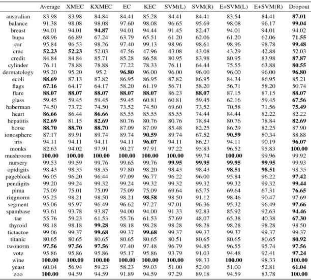
We show test accuracy performances of all fusion methods for 38 datasets in Table 4.1. The results in Table 4.1 will be used as an empirical dataset for fusion method selection in the next section. In Table 4.1, EC and KEC denotes Eigenclassifiers [5] and kernelized version [19] respectively, XMEC and KXMEC denotes Extended Multimodal Eigenclassifiers and kernelized version respectively, SVM(L) denotes Support Vector Machines with linear kernel, E+SVM(R) denotes Eigen Support Vector Machines [19] with RBF kernel. We give a more through comparison of the fusion methods below, but, a first look at Table 4.1, shows that the Dropout method performs the best for most datasets.KXMEC and KEC seems to perform better than XMEC, and XMEC is better than EC. However, in agreement with the results stated in [5], Average seems to perform as well as those four methods.

In order to compare the fusion methods across all the datasets, we perform a number of tests. First, we show pairwise comparison of the ensemble methods in Table 4.2. Each cell entry in Table 4.2 shows the number of data sets on which the algorithm

i is the overall winner. Keeping in mind that these results are claimed only for this collection of datasets, we see that the Dropout method has the overall best performance. Combination methods that include SVM perform the worst. On the second row of the table, we compare only the XMEC, KXMEC, KEC and EC methods. The KXMEC and KEC methods perform better than the XMEC and EC. According to the third row of this table, XMEC performs better than EC on more datasets.

We also applied Wilcoxon signed-rank test [24], to see if there is a significant difference between two methods. Wilcoxon signed-rank test rejects the null hypothesis ("the median of the ranking of the differences of performances is 0") at the 6% significance level. In order to compare all ensemble methods on all 38 datasets, we applied nonparametric Friedman test [24], to see if any method is significantly different from other methods. The average rank of each ensemble method is shown in Table 4.3. The foundρ value is smaller than 0.05, which means Friedman test rejects

the null hypothesis that all ensembles are the same, so we continue with a post-hoc

Table 4.1: Test accuracies of fusion methods on AYSU dataset collection Average XMEC KXMEC EC KEC SVM(L) SVM(R) E+SVM(L) E+SVM(R) Dropout australian 83.98 83.98 84.84 84.41 85.28 84.41 84.41 83.54 84.41 87.01 balance 91.38 98.08 98.08 97.60 98.08 96.65 95.69 98.08 96.17 99.04 breast 94.01 94.01 94.87 94.01 94.44 91.45 82.47 94.01 94.01 94.02 bupa 68.96 66.89 67.24 63.79 65.51 61.20 62.06 61.20 62.06 71.55 car 95.84 96.53 98.26 97.40 99.13 98.96 98.61 98.96 98.78 99.48 cmc 52.23 52.23 52.03 47.56 47.96 43.08 43.08 43.29 42.88 52.03 credit 84.84 84.84 85.71 85.28 86.58 80.95 83.98 80.95 83.98 87.87 cylinder 76.11 78.88 78.88 77.22 78.33 76.11 64.44 75.55 63.88 80.55 dermatology 95.20 95.20 95.2 96.80 96.00 96.00 96.00 96.00 96.00 96.80 ecoli 88.69 87.13 87.82 86.95 86.95 87.82 86.95 84.34 86.95 85.21 flags 67.16 64.17 64.17 58.20 61.19 56.71 58.20 56.71 58.20 50.74 flare 88.07 88.07 88.07 88.07 88.07 86.23 88.07 87.15 87.15 88.07 glass 59.45 59.45 59.45 59.45 60.81 60.81 59.45 62.16 59.45 67.56 haberman 74.50 73.72 74.50 73.52 74.50 69.60 73.52 70.58 71.56 75.49 heart 86.66 86.44 86.66 85.55 85.55 85.55 74.44 84.44 82.22 82.22 hepatitis 82.69 81.15 82.69 80.76 80.76 80.76 78.84 80.76 78.84 82.69 horse 88.70 88.70 88.70 87.09 87.09 85.48 82.25 86.29 82.25 87.90 ionosphere 87.17 89.91 89.74 89.74 90.59 89.74 67.52 90.59 80.34 88.88 iris 94.11 94.11 94.11 94.11 96.07 94.11 86.27 94.11 90.19 96.07 monks 82.63 94.02 97.91 90.27 97.91 97.22 95.83 96.52 95.83 100.00 mushroom 100.00 100.00 100.00 100.00 100.00 100.00 99.74 100.00 99.96 99.92 nursery 99.53 99.59 99.76 99.65 99.76 99.95 99.95 99.95 99.95 99.93 optdigits 98.43 98.35 98.35 97.80 98.20 98.43 98.43 98.51 98.51 98.35 pageblock 96.05 96.20 96.44 97.09 96.77 96.22 96.00 95.84 96.22 97.42 pendigits 99.20 99.24 99.32 99.24 99.32 99.32 99.32 99.32 99.32 99.44 pima 75.09 75.01 75.09 75.09 75.09 69.64 65.75 69.64 67.31 76.65 ringnorm 95.25 98.21 98.50 98.21 98.58 98.50 91.12 98.46 90.47 97.69 segment 95.06 95.97 96.49 96.62 97.27 97.01 96.36 95.32 96.49 97.66 spambase 93.61 93.78 93.87 94.00 94.00 91.33 92.83 85.92 92.63 94.46 tae 55.76 59.23 61.53 55.76 61.53 57.69 48.07 65.38 40.38 67.30 thyroid 98.18 98.18 99.28 98.18 98.28 98.28 98.28 98.28 98.28 98.50 tictactoe 99.06 99.37 99.68 99.37 99.68 99.37 99.37 99.37 99.37 99.37 titanic 80.65 80.65 80.65 80.65 80.65 80.51 80.65 80.65 80.65 80.92 twonorm 97.56 97.56 97.56 97.40 97.48 96.79 94.85 96.55 95.74 97.56 vote 95.86 95.86 95.86 95.17 95.86 93.79 91.03 94.48 92.41 97.24 wine 100.00 100.00 100.00 100.00 100.00 100.00 98.33 100.00 98.33 100.00 yeast 60.04 56.94 59.23 58.23 59.03 51.00 52.00 51.00 52.81 61.04 zoo 100.00 94.59 94.59 91.89 94.59 97.29 89.18 94.59 83.78 100.00

Table 4.2: Number of experiments each method performed the best

Average XMEC KXMEC EC KEC SVM(L) SVM(R) E+SVM(L) E+SVM(R) Dropout

All 11 6 10 4 7 3 2 5 2 25

Eigen 12 27 8 23

XMEC vs EC 27 21

Tukey’s test to determine which pairs of ensembles are significantly different, and which are not. Figure 4.1 shows the average ranks of each ensemble and the range between vertical green dots is the critical value according to Tukey’s test. Figure 4.1 shows that, Extended Multimodal Eigenclassifiers and kernelized version, Kernelized Eigenclassifiers, Dropout and Dropout + ES (early stop) methods (shown in red) are significantly different from the least accurate ensemble method SVM(R) (shown in blue). The Dropout method is significantly different from the Average method, while the other methods are not.

We developed the XMEC ensemble method so that the estimator variance would be reduced. In Figure 4.2, we compare variances of estimators according to Equation

Table 4.3: Average rank of each ensemble method

Average XMEC KXMEC EC KEC SVM(L) SVM(R) E+SVM(L) E+SVM(R) Dropout + ES Dropout 6.18 6.03 4.21 6.40 4.27 6.71 8.40 6.88 8.10 5.43 3.34 2 3 4 5 6 7 8 9 10 Dropout Dropout + ES E+SVM(R) E+SVM(L) SVM(R) SVM(L) KEC EC KXMEC XMEC Average Ensemble Methods Mean Ranks

Figure 4.1: The ensemble methods shown in red are significantly different than the ensemble method shown in blue according to Tukey’s critical value range shown by the vertical blue line.

0 20 40 60 80 100 120 australianbalance

breastbupacar cmccredit cylinder dermatology

ecoli flags flareglass haberman heart hepatitishorse ionosphere iris monks mushroom nurseryoptdigits pageblockpendigits pima ringnormsegment_spambase

tae thyroid_tictactoetitanic

twonorm vote wineyeast zoo

Variance

Figure 4.2: Variance of estimators for Eigenclassifiers (red) and Extended Multimodal Eigenclassifiers (blue).

(4.4), for Eigenclassifiers (EC) and Extended Multimodal Eigenclassifiers (XMEC). We show the variances on 38 datasets from AYSU [1]. The variance is computed according to1TCov(d)1=1TCov(UTXv)1, where1is a vector whose all elements are 1s. Note that this expression corresponds to summing all entries in the covariance matrix Cov(d). According to this figure, the variances for the XMEC method are lower than the variances for the EC method, which could be the explanation for the better performance of the XMEC method.

4.5 Criteria for Fusion Method Selection

In the previous section, we presented accuracy results obtained using different fusion methods. In this section, based on a number of measurements on the available base classifier outputs, we aim to determine the suitable fusion method(s) for a particular dataset.

Previous studies [11,20] considered diversity and accuracy of classifiers to characterize the classifier ensemble used for classifier fusion. We consider five different diversity measures, namely, Q statistics, correlation coefficient ρ, disagreement measure,

double-fault measure and the entropy [20]. In this thesis, in addition to these measures, we introduce a metric, which is based on the distribution of the eigenvalues of the output matrix of base classifiers.

Table 4.1 shows that Eigenclassifiers method works best for Dermatology, Flare, Mushroom and Wine datasets, so we can use the average of the diversity measures of these datasets as a representation of Eigenclassifiers method, and the same is true for average eigenvalue distribution representation.

4.5.1 Average Eigenvalue Distributions and Diversity Metrics

If the base classifier outputs are highly correlated, we can approximate the output matrix with a fewer eigenvalue, eigenvector pair and as the number of pairs reduce, the first normalized eigenvalue will be closer to 1, and if the base classifiers are not correlated eigenvalues will be distributed more uniformly. We are going to use this observation first to identify the features of ensemble methods and secondly we are going to use eigenvalues of each dataset with the diversity metrics defined below as an input to a decision tree to see if we can learn rules that associates diversity and the accuracy of ensemble methods.

We use 5 diversity metrics, namely, Q statistics, correlation coefficientρ, disagreement

measure, double-fault measure and the entropy, as defined in (Kuncheva et al. 2001) [20]. Please see [20] for more details on these metrics.

When comparing the classifiers i and k, let N00,N11,N01,N10 be the number of instances for which both classifiers were wrong, both classifiers were right, classifieri

was wrong andkwas right, and classifieriwas right andkwas wrong, respectively. Let

Lbe the number of base classifiers and defineyj,i=1, if the base classifiericorrectly

recognizes the instance x_j. I(x_j) = ∑L i=1

y_j,i is the number of classifiers that correctly recognizexj.

Based on these definitions, diversity metrics are defined as follow: Q statistics: Q_i,k= N 11_N00_−N01_N10 N11N00+N01N10 (4.24) Q_av= 2 L(L−1) L−1

∑

i=1 L

∑

k=i+1 Q_i,k (4.25) Correlation coefficientρ: ρi,k= N11N00−N01N10 p (N11+N10)(N01N00)(N11+N01(N10+N00)) (4.26) ρav= 2 L(L−1) L−1

∑

i=1 L

∑

k=i+1 ρi,k (4.27) Disagreement measure: Dis_i,k= N01+N10 N11_+N10_+N01_+N00 (4.28) Dis_av= 2 L(L−1) L−1

∑

i=1 L

∑

k=i+1 Dis_i,k (4.29) Double-fault measure: DF_i,k= N 00 N11_+N10_+N01_+N00 (4.30) DFav= 2 L(L−1) L−1

∑

i=1 L

∑

k=i+1 DF_i,k (4.31) Entropy measure: E = 1 N N

∑

j=1 1 (L− dL/2e)min(I(xj),L−I(xj)) (4.32)

In order to identify the features of ensemble methods, first we note the datasets on which each method gave the best results using Table 4.1 and then we average the eigenvalue distributions of each group of datasets. We also followed the same

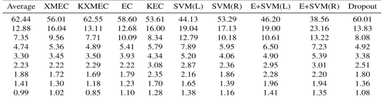
Table 4.4: Average eigenvalue distribution

Average XMEC KXMEC EC KEC SVM(L) SVM(R) E+SVM(L) E+SVM(R) Dropout 62.44 56.01 62.55 58.60 53.61 44.13 53.29 46.20 38.56 60.01 12.88 16.04 13.11 12.68 16.00 19.04 17.13 19.00 23.16 13.83 7.35 9.56 7.71 10.09 8.34 12.79 10.18 10.61 13.22 8.08 4.74 5.36 4.89 5.41 5.79 7.89 5.95 6.50 7.23 4.92 3.30 3.45 3.50 3.93 4.34 5.20 4.06 4.90 5.39 3.38 2.23 2.22 2.29 2.22 3.08 2.87 2.36 2.95 3.01 2.51 1.88 1.72 1.69 1.79 2.35 2.16 1.86 2.28 2.20 1.80 1.41 1.30 1.18 1.23 1.70 1.65 1.39 1.96 1.94 1.36 0.99 1.02 0.85 1.10 1.28 1.38 1.16 1.41 1.35 1.08

procedure to identify the features of ensemble methods using diversity metrics instead of eigenvalue distributions. Average eigenvalue distributions and diversity metrics of each fusion method is given in Table 4.4 and Table 4.5. According to these tables and the empirical dataset we studied on, three methods SVM(L), E+SVM(L) and E+SVM(R) differs from other methods on non-correlated datasets (more uniform distribution on the first two eigenvalues also, lower Q statistics and Correlation coefficient). We also used a decision tree to learn simple rules that associates diversity and accuracy of ensemble methods. Diversity is defined by eigenvalue distributions and the diversity metrics defined above. Accuracy is defined by normalizing each row of Table 4.1 into range [0-1] and specifying a threshold, which we selected 0.8, to turn Table 4.1 into a label matrix. We measured the number of mis predictions by leave-one-out cross-validation as our evaluation method. The performance averaged over 38 datasets was two misprediction among eleven methods. The rules extracted by the Decision Tree are given in Fig 4.3.

Table 4.5: Average divergence metrics

Average XMEC KXMEC EC KEC SVM(L) SVM(R) E+SVM(L) E+SVM(R) Dropout Q statistic 0.588 0.514 0.630 0.357 0.505 0.126 0.577 0.336 0.339 0.595 Correlation coeff 0.370 0.355 0.404 0.292 0.292 0.082 0.446 0.144 0.082 0.346 Disagreement 0.165 0.110 0.107 0.110 0.151 0.172 0.155 0.173 0.257 0.210 Double-fault 0.065 0.031 0.037 0.029 0.036 0.014 0.058 0.018 0.020 0.100 Entropy 0.221 0.133 0.136 0.130 0.195 0.210 0.192 0.212 0.312 0.288 29