University of California, Berkeley
U.C. Berkeley Division of Biostatistics Working Paper Series
Year Paper
Statistical Learning of Origin-Specific
Statically Optimal Individualized Treatment
Rules
Mark J. van der Laan
∗Maya L. Petersen
†∗Division of Biostatistics, School of Public Health, University of California, Berkeley,
†Division of Biostatistics, School of Public Health, University of California, Berkeley,
This working paper is hosted by The Berkeley Electronic Press (bepress) and may not be commer-cially reproduced without the permission of the copyright holder.
http://biostats.bepress.com/ucbbiostat/paper210 Copyright c2006 by the authors.
Statistical Learning of Origin-Specific
Statically Optimal Individualized Treatment
Rules
Mark J. van der Laan and Maya L. Petersen
Abstract
Consider a longitudinal observational or controlled study in which one collects chronological data over time on n randomly sampled subjects. The time-dependent process one observes on each randomly sampled subject contains time-dependent covariates, time-dependent treatment actions, and an outcome process or single final outcome of interest. A statically optimal individualized treatment rule (as introduced in van der Laan, Petersen & Joffe (2005), Petersen & van der Laan (2006)) is a (unknown) treatment rule which at any point in time conditions on a user-supplied subset of the past, computes the future static treatment regimen that maximizes a (conditional) mean future outcome of interest, and applies the first treatment action of the latter regimen. In particular, Petersen & van der Laan (2006) clarified that, in order to be statically optimal, an individualized treatment rule should not depend on the observed treatment mechanism. Petersen & van der Laan (2006) further developed estimators of statically optimal individualized treatment rules based on a past capturing all confounding of past treatment his-tory on outcome. In practice, however, one typically wishes to find individualized treatment rules responding to a user-supplied subset of the complete observed his-tory, which may not be sufficient to capture all confounding. The current article provides an important advance on Petersen & van der Laan (2006) by developing locally efficient double robust estimators of statically optimal individualized treat-ment rules responding to such a user-supplied subset of the past. However, failure to capture all confounding comes at a price; the static optimality of the resulting rules becomes origin-specific. We explain origin-specific static optimality, and discuss the practical importance of the proposed methodology. We further present the results of a data analysis in which we estimate a statically optimal rule for switching antiretroviral therapy among patients infected with resistant HIV virus.
1
Introduction.
Consider a longitudinal observational or controlled study in which one collects data over time on n randomly sampled subjects. The time-dependent process one observes on each randomly sampled subject contains time-dependent co-variates, time-dependent treatment actions, and either an outcome process or a single final outcome of interest. This time-dependent process is a ran-dom variable defined by the experiment which ranran-domly samples a subject and subsequently measures this time-dependent process. In statistical learn-ing one refers to this random variable as the experimental unit. The statistical question we are concerned with can be stated as follows: Can we use data con-sisting of n such time-dependent processes to estimate a treatment rule that responds to a user-supplied subset of a subject’s measured history in such a way that it aims to maximize the mean outcome of interest? Treatment rules of this type, which respond to individual covariates, are called individualized treatment rules or dynamic treatment regimes.
In order to address the question of interest, we focus on estimation of statically optimal individualized treatment rules. A statically optimal indi-vidualized treatment rule is an (unknown) treatment rule which at any point in time conditions on a user-supplied subset of the past, computes the future static treatment regimen maximizing a (conditional) mean future outcome of interest, and applies the first treatment action of the latter regimen. We re-fer to this treatment rule as a statically-optimal individualized treatment rule, to distinguish it from an optimal dynamic treatment regime as modelled in Murphy (2003) and Robins (2003).
We first introduced statically optimal individualized treatment rules in our article van der Laan et al. (2005) in which we introduced (observed) history-adjusted marginal structural models (HA-MSM). However, as made explicit in Petersen et al. (2006), the optimality of rules estimated by HA-MSM can depend on the treatment mechanism of the observed data, and as a result, the HA-MSM-derived rule can fail to select the optimal future treatment plan (given individual covariate values) if applied to an equivalent population with a different observed treatment mechanism. Dependence on observed treatment mechanism implies, in particular, that the rule can fail to select the statically optimal treatment at each time point in the setting where the rule itself has been applied to the population beginning at baseline (as, for example, would occur if the rule were tested in a clinical trial). As a result, Petersen et al. (2006) refine the definition of static optimality to specify that a statically optimal rule must not depend on observed treatment mechanism. They further point out that HA-MSM-derived rules are only truly statically optimal if the covariates in the history-adjusted marginal structural model are sufficient to capture all confounding of past treatment on outcome.
The statically optimal rules discussed by Petersen et al. (2006) have the at-tractive property that they select the optimal future treatment planregardless
of how past treatment has been assigned. As a result, these rules will re-tain their static optimality if applied to an exchangeable population that has been following the rule in question (as would occur in the context of a clini-cal trial) or if applied to an exchangeable population that has been following some unknown treatment mechanism (as could occur in the course of clinical practice). In order to achieve this generality, however, the statically optimal rules must incorporate sufficient covariate history to control for confounding of past treatment history on outcome.
Due to limited resources, practical sensibility, and reliability, clinical tri-als will be forced to focus on candidate individualized treatment rules which only respond to a small number of user-supplied bio-markers or other rele-vant measurements. The current article provides an important advance by presenting models and corresponding locally efficient double robust estima-tors of individualized treatment rules responding to a user-supplied subset of a subject’s past. However, failure to incorporate sufficient covariates to con-trol for confounding has a price: the static optimality of the resulting rules isorigin-specific. In other words, the individualized treatment rules described in this paper retain their optimality only in settings where the population has been following the rule itself beginning at baseline (or in other words, a since a specified origin). Thus the origin-specific statically optimal rules described in this paper are appropriate for evaluation in the context of a clinical trial, but not for application to an individual who has been following an unknown past treatment mechanism, as may occur in the context of clinical practice.
1.1
Organization of article.
In Section 2 we define the observed data and a statistical framework/model for the data generating distribution in which we formally state the statistical learning problem to be addressed. In particular, we define the origin-specific statically optimal treatment rule. We introduce a novel parameter, the coun-terfactual history-adjusted mean outcome, which represents a mean outcome conditional on a user-supplied subset of the past in the counterfactual world in which each subject follows a particular static treatment regimen. We then show that the counterfactual history-adjusted mean implies our desired origin-specific statically optimal rule. We further demonstrate the identifiability of the statically optimal individualized treatment rule. Our model corresponds with only modelling the counterfactual history-adjusted mean outcome, while leaving all nuisance parameters unspecified. In Section 3 we derive the class of all estimating functions in this model for the data generating distribution, which are orthogonal to the nuisance parameters and thereby result in robust
estimation procedures. These estimating functions for the parameter of inter-est are indexed by nuisance parameters: the treatment mechanism, and the conditional distributions of the covariates given the past. However, due to the orthogonality property of these estimating functions, they remain unbi-ased if one (not both) of these two nuisance parameters is misspecified. In the literature these estimating functions are referred to as double robust in-verse probability of treatment weighted (IPTW) estimating functions (van der Laan and Robins (2003)). By assuming models for these two nuisance pa-rameters, which represent factors in the likelihood of the observed data, and estimating them accordingly with maximum likelihood procedures, we obtain double robust IPTW estimators of the origin-specific statically optimal indi-vidualized treatment rules. In Section 4 we discuss statistical inference. In Section 5 we review conditions under which the origin-specific statically opti-mal treatment rule estimated using the counterfactual history-adjusted mean parameter, as presented in this paper, is equivalent to the statically optimal rule defined by Petersen et al. (2006). Section 6 presents the results of a data analysis drawn from the treatment of patients infected with resistant HIV. We estimate origin-specific statically optimal individualized rules for deciding when to switch antiretroviral therapy regimen among patients with incom-plete virologic suppression due to resistant virus. Section 7 discusses various generalizations of practical interest.
2
The origin-specific statically optimal
indi-vidualized treatment rule and
counterfac-tual history-adjusted mean.
We adopt the counterfactual causal inference framework in order to formally define the origin-specific statically optimal individualized treatment rule, and the counterfactual history-adjusted mean outcome on which it is based, as parameters of the data generating distribution.
2.1
The statistical framework.
The observed data structure on a randomly sampled subject is defined as a missing data structure on the set of treatment-specific time-dependent processes, where each treatment-specific process represents the counterfactual data we would have observed on the subject, if, possibly contrary to the fact, the sub-ject would have followed that particular treatment regimen. In addition, we make the sequential randomization assumption (defined below), allowing us to identify the probability distribution of the counterfactual processes, and
thereby allowing us to learn causal parameters of interest from the observed data.
Representation of the observed data as a missing data structure.
The chronological data structure observed on a randomly sampled subject/ experimental unit is given by
O = (L(0), A(0), L(1), A(1), . . . , L(T −1), A(T −1), L(T)),
whereL(t) is data collected at timet,A(t) is treatment at timetassigned after
L(t), T ≤ K + 1 is a fixed end-point or a random end-point such as death and K + 1 denotes a maximal follow up time. It is assumed that for each subject and each possible treatment regimen ¯a = (a(0), . . . , a(K))∈ A there exists a process L¯a = L¯a(0), . . . , L¯a(T¯a), and that the observed process L on
the subject is the treatment-specific process indexed by the treatment regimen the subject actually took: L=LA¯. HereAdenotes the support of the random
treatment process ¯A = (A(0), . . . , A(K)). Thus, we define a collection of treatment-specific time-dependent processes (La¯(t) : 0 ≤t ≤Ta¯), stopped by
some possibly random stopping timeT¯a, and indexed by a treatment regimen
¯
a= (a(0), . . . , a(K)).
We assume that there is an experiment resulting in the observation of all these random processes, and we denote this random variable with X = (L¯a :
¯
a∈ A) (in the censored data literature,X is often referred to as the full data). LetPX0 denote the probability distribution of this collection X of
treatment-specific processes. It is assumed that L¯a(t) = L¯a(t−1)(t), where we use the
notation ¯a(t) = (a(0), . . . , a(t)). The latter assumption is implied by the time-ordering assumption thatA(t) occurs afterL(t) and beforeL(t+ 1). We make the convention that La¯(t) = La¯(min(t, T¯a)) and A(t) = A(min(t, T −1)), so
that these processes are also defined after the stopping time. Let Y¯a(t) be a
treatment-specific outcome process, andS¯a(t) denote the components ofL¯a(t)
on which the individualized treatment rule is based. It is assumed that S¯a(t)
includes the stopping time indicator process I(T¯a ≤ t). To conclude, the
observed data structureO on a randomly sampled subject can be represented as
O = ( ¯A, LA¯),
or equivalently,
O = (L(0), A(0), LA(0)(1), A(1), . . . , LA¯(T−2)(T −1), A(T −1), LA¯(T−1)(T)),
where T =TA¯. Thus the observed random process O is a missing data
struc-ture on the full data strucstruc-ture X.
LetG0(· |X) denote the conditional probability distribution of ¯AgivenX,
which is called the treatment mechanism since it determines how treatment is assigned. We note that the observed data structure O is a random variable
with a probability distribution PPX0,G0 implied by PX0 and G0(· | X). We
assume that we observe n i.i.d. copies O1, . . . , On of this random variable
O ∼PPX0,G0.
Sequential randomization assumption. In order to be able to identify parameters of the probability distribution of X from the probability distribu-tion ofO, we assume the coarsening at random assumption on the missingness/ treatment mechanism G0(· |X). That is,
g0(¯a(T¯a−1)|X) ≡ TY¯a−1 t=0 Pr(A(t) =a(t)|A¯(t−1) = ¯a(t−1), X) = TY¯a−1 t=0 Pr(A(t) =a(t)|A¯(t−1),L¯A¯(t)).
In the context of causal inference this is often referred to as the sequential randomization assumption.
In the following sections we first define the origin-specific statically optimal treatment rule. We then show that this rule identified by the counterfactual history-adjusted mean, a parameter of PX0.
2.2
The origin-specific statically optimal individualized
treatment rule.
We begin by defining counterfactuals indexed by individualized treatment rules. For a given rule d with treatment assignment at time t a function of
¯
L(t), the corresponding counterfactual processLdis a random variable defined
by the deterministic function of the collection of treatment-specific processes
X = (La¯ : ¯a) and the rule d given by Ld≡L¯a(d,X), where ¯a(d, X) is the
treat-ment vector assigned by ruled for a subject with full data structureX. Thus, counterfactual processes/random variables Ld indexed by any individualized
treatment ruled are also well defined, given our definition of static treatment regimen-specific processes L¯a for all ¯a.
Using this definition of a counterfactual covariate process indexed by an individualized treatment rule, we provide the following definition of an origin-specific statically optimal treatment rule. Yd(t, m) is a future rule-specific
(counterfactual) outcome such as, for example,Yd(t+m) for some user-supplied
integerm ≥0. In order to keep some generality, we allow this outcomeYd(t, m)
to be any function of the future outcome process (Yd(s) :s≥t) starting at time
t, indexed by a scalarm. We letdtdenote the function assigning the treatment
decision under rule d at time t, ¯dt = (d0, d1, . . . , dt) and a(t) denote a future
static treatment regimen beginning at time t,a(t) = (a(t), a(t+ 1), . . . , a(K)). We use K(m) to denote the last time point t for which Y(t, m) is defined.
For example, if Y(t, m) = Y(t +m), then Y(t, m) is only defined for t = 0, ..., K(m) =K+ 1−m.
Note that T represents a stopping time that defines the end of the full data of interest, rather than simply a censoring event acting as an additional missingness mechanism on the full data. For example, T may represent death or a specific failure time of interest; in such cases T will generally be incor-porated explicitly in the outcome. For example, if T represents death, the outcome of interest may be survival; i.e. Y(t, m) = I(T > t + m). Al-ternatively, the outcome of interest might include both T and a covariate process. For example, a researcher interested in disease progression might consider an outcome that reflects both whether a patient is still alive, and if so, whether a biomarker of interest (W) has crossed a given threshold (th); i.e. Y(t, m) = I(T > t +m)I(W(t +m) > th). Note that if T represents death, then defining the outcome using only a covariate process, without in-corporating T explicitly, will result in a covariate outcome defined for time points following a patient’s death (specifically, an outcome reflecting the last measurement of the covariate prior to death). In most cases such an outcome will not be of interest. An alternative incorporation of T into the parameter of interest is presented in the data example in Section 6.
Definition 1 Below we define an origin-specific statically optimal dynamic treatment rule
¯
dK ≡d¯K( ¯Sd(K)) = (d0(S(0)), d1( ¯Sd(1)), . . . , dK( ¯Sd(K))),
where each function S¯d(t) → dt( ¯Sd(t)) describes how A(t) is assigned in
re-sponse to S¯d(t) for all t= 0, . . . , K.
This rule d is defined by the following algorithm:
a∗(0|S(0)) = arg max a(0) E(Y0,a(0) |S(0)) d0 ≡a∗(0|S(0))(1) a∗(1|S¯ d0(1)) = arg max a(1) E(Yd0,a(1) | ¯ Sd(1)) d1 ≡a∗(1|S¯d(1))(1) a∗(t |S¯ d(t)) = arg max a(t) E(Yd¯t−1,a(t) | ¯ Sd(t)) dt =a∗(t |S¯d(t))(1), t = 2, . . . , K(m),
where Yd¯t−1,a(t) ≡ Yd¯t−1,a(t)(t, m) is the counterfactual random variable
corre-sponding to following the treatment rule d from time0 to time t−1, and then static treatment regimen a(t). Similarly, S¯d(t)≡S¯d¯t−1(t) is the counterfactual
random variable corresponding to following the treatment rule d from time point 0 to time t−1. a∗(t |S¯
d(t))(1) is used to denote the first component of
the optimal static treatment regimen a∗(t |S¯
d(t)).
For time points t =K(m) + 1, ..., K, the rule dt assigns the next action of
the static regimen
a∗(K(m)|S¯d(K(m))) = arg max
a(K(m))E(Yd¯K(m)−1,a(K(m)) |S¯d(K(m)))
Note that the origin-specific statically optimal rule must assign treatment deterministically at every time point. Thus, while in many settings there may be several choices of a(t|S¯d(t)) that optimize the expected outcome (i.e. the
arg maxa(t) is not unique), in this case the user must specify a deterministic
way of choosing between these choices. Further, note that the rule defines a treatment decision for each time point up till time K for each subject, even though the full data of interest for some subjects may end at time T. However, asT denotes the end of the full data for a subject, treatment decisions occurring after T will not be relevant for the counterfactuals of interest.
The origin-specific statically optimal treatment rule of Definition 1 satisfies the following property: it selects, at each time pointt, the initial treatment of the futurestatic regimen (a(t)) which optimizes the expected outcomeY(t, m), given the history ¯S(t), in the world where treatment up till that time point corresponds to following the statically optimal treatment rule d (and thus
¯
S(t) = ¯Sd(t) and the counterfactual outcome is also indexed by ¯dt−1). We
specify that the rule isorigin-specific to clarify that, if applied to a population with an identical full data generating distribution, the rule will assign the optimal future static regimen at each time point if past treatment (beginning at baseline, or the origin) has been assigned according to the rule itself. Thus the rule is appropriate for evaluation in the context of a clinical trail, where the rule itself is applied beginning at enrollment. The origin-specific statically optimal rule can be distinguished from the statically optimal rule defined by Petersen et al. (2006), in that the latter selects the optimal future static regimen at each time point regardless of how past history has been assigned.
2.3
The counterfactual history-adjusted mean outcome
and corresponding treatment rule.
In this section, we show that the origin-specific statically optimal treatment rule is a function of the counterfactual history-adjusted mean outcome. We first define the counterfactual history-adjusted mean outcome as a parameter of the full data generating distribution, and define an individualized treatment rule based on this parameter. Next, we show that this treatment rule is equiv-alent to the origin-specific statically optimal treatment rule, and thus that the counterfactual history-adjusted mean outcome identifies the rule of interest.
The counterfactual history-adjusted mean outcome is defined as
E(Y¯a(t−1),a(t)(t, m)|S¯¯a(t−1)(t)), (1)
This counterfactual history-adjusted mean outcome provides us with the fol-lowing individualized treatment rule:
Definition 2 Define
θ0(t, a(t)|¯a(t−1),s¯(t))≡E(Ya¯(t−1),a(t) |S¯a¯(t−1)(t) = ¯s(t)).
We define the following treatment rule:
¯
dK(θ0)( ¯S(K)) = (d0(S(0)), d1( ¯S(1)), . . . , dK( ¯S(K))),
where each functionS¯(t)→dt( ¯S(t))describes howA(t)is assigned in response
to S¯(t) for all t = 0, . . . , K.
This rule d¯K(θ0) is defined by the following algorithm applied to S¯(K) =
(S(0), . . . , S(K)): a∗(0|S(0)) = arg max a(0) θ(0, a(0) |S(0)) d0(S(0))≡a∗(0|S(0))(1) a∗(1|S¯(1)) = arg max a(1) θ(1, a(1) |d0(S(0)), ¯ S(1)) d1( ¯S(1))≡a∗(1|S¯(1))(1) a∗(t|S¯(t)) = arg max a(t) θ(t, a(t)| ¯ dt−1( ¯S(t−1)),S¯(t)) dt( ¯S(t)) =a∗(t|S¯(t))(1), t = 2, . . . , K(m).
Here we use the notation d¯t−1( ¯S(t−1)) ≡(d0(S(0)), d1( ¯S(1)), . . . , dt−1( ¯S(t−
1))) for the first t−1 components of the dynamic treatment rule d applied to
¯
S(t−1), where we note thatd¯t( ¯S(t))corresponds to a specific ¯a(t). As above,
a∗(t | S¯(t))(1) denotes the first component of the optimal static treatment
regimen a∗(t | S¯(t)). And as above, for time points t = K(m) + 1, ..., K, the
rule dt assigns the next action of the static regimen
a∗(K(m)|S¯(K(m))) = arg max
a(K(m))θ(t, a(K(m))|
¯
dK(m)−1( ¯S(K(m)−1)),S¯(K(m)))
We now show that, once we condition on the covariates on which the treat-ment rule depends, E(Y¯a(t−1),a(t) | S¯¯a(t−1)(t) = ¯s(t)) is equal to E(Yd¯t−1,a(t) |
¯
Sd(t) = ¯s(t)) at a particular ¯a(t −1), and thus the origin-specific statically
optimal regimen of interest (Definition 1) is identified by applying Definition 2 to the counterfactual history-adjusted mean (1). This is because, as shown in Definition 1, given ¯s(t), the origin-specific statically optimal treatment rule applied at time t corresponds to a deterministic choice of a(t), t = 0, ..., K. We presents these results formally as a Lemma:
Lemma 1 Define
θ0(t, a(t)|a¯(t−1),s¯(t))≡E(Ya¯(t−1),a(t)(t, m)|S¯a¯(t−1)(t) = ¯s(t)),
Given a dynamic treatment rule S¯(K)→d( ¯S(K)), we have
E(Yd¯t−1a(t)(t, m)|S¯d(t) = ¯s(t)) =θ(t, a(t)|¯ad¯t−1(t−1),s¯(t)), (2)
where Yd¯t−1a(t)(t, m) is the counterfactual random variable corresponding with
following rule d from time 0 till t−1, and subsequently, following the static treatment regimen a(t). Note that Yd¯t−1a(t)(t, m) is a random variable defined
as a deterministic function of X, the rule d, and static treatment a(t). We use ¯ad¯t−1 to denote the treatment history (through time t) corresponding to
applying rule d to ¯s(t−1).
Proof Given ¯Sd(t) = ¯Sd¯t−1(t) = ¯s(t), we have that ¯dt−1 = (a(0), . . . , a(t−1))
for some fixed ¯ad¯t−1(t −1) defined by ¯s(t). Thus, given ¯Sd(t) = ¯s(t), with
probability equal to 1 we haveYd¯t−1a(t)(t, m) = Y¯adt¯−1(t−1)a(t)(t, m) and ¯Sd(t) =
¯
S¯adt¯−1(t−1)(t): that is, counterfactuals indexed by dynamic treatment regimens
are identical to counterfactuals indexed by a corresponding static treatment regimen, which proves the result (2). 2
Origin-specific static optimality ofd(θ0). The importance of this identity
(2) is established as follows. Suppose that the treatment decisionsA(0), . . . , A(t−
1) have been assigned according to the treatment rule d = d(θ0) so that A(0) = d0(S(0)), A(1) = d1( ¯Sd(1)), . . . , A(t−1) = dt−1( ¯Sd(t−1)), and that
we are now confronted with making a treatment decision at time t: thus, we are given the treatment past ¯A(t−1) = ¯dt−1( ¯Sd(t−1)) and covariate past
¯
Sd(t) in the world in which we have been applying rule d = d(θ0). We want
to show that the origin-specific statically optimal treatment decision at time
t, given ¯Sd(t), is now precisely given by dt( ¯Sd(t)) with d=d(θ0). The
origin-specific statically optimal treatment decision at time t, given ¯Sd(t), is defined
by optimizing the wished expected outcome E(Yd¯t−1a(t)(t, m) | S¯d(t) = ¯s(t))
over all static future treatment regimens a(t), and carrying out the first com-ponent of this latter treatment regimen. By the previous lemma applied to
d = d(θ0), it follows that at time t, optimizing the wished expected outcome
E(Yd¯t−1a(t)(t, m) | S¯d(t) = ¯s(t)) over all statically future treatment regimens
a(t) is equivalent with optimizing θ0(t, a(t) | a¯d(t−1),s¯(t)) over a(t). This
proves that indeed the origin-specific statically optimal treatment decision at time t, given ¯Sd(t), is now precisely given by dt( ¯Sd(t)). Thus, if treatment
decisions are assigned deterministically according to ruled(θ0), then it follows
that at each point in time t, given the observed ¯S(t) = ( ¯Sd(t)) = ¯s(t), our
regimen maximizing the mean outcome of Yd¯t−1a(t)(t, m), given ¯S(t) = ¯s(t),
over all future static treatment regimens a(t). This proves that indeed the rule d(θ0) is an origin-specific statically optimal treatment rule, and thus that estimates of this ruled(θ0) are potential candidates for treatment regimens to
be evaluated in clinical trials.
In this section we have established that the counterfactual history-adjusted meanθ0 identifies the origin-specific statically optimal dynamic treatment rule,
and illustrated why such a rule is of interest. In the next section we discuss estimation of θ0, and thus estimation of the origin-specific statically optimal dynamic treatment rule d(θ0).
2.4
A model for the counterfactual history-adjusted mean.
In order to deal with the curse of dimensionality, we will assume a model for our parameter of interestθ(PX)(t, a(t)|a¯(t−1),s¯(t)) =EPX(Ya¯(t−1)a(t)(t, m)|
¯
S¯a(t−1)(t) = ¯s(t)) of PX:
θPX(t, a(t)|¯a(t−1),¯s(t)) =mβ(PX)(t, a(t)|¯a(t−1),¯s(t)) (3) for some parametrization (mβ :β) indexed by a Euclidean parameter β. Let
β0 = β(PX0) denote the true parameter value of β. Note that we could also
extend the definition of this parameter to the nonparametric model consisting of all full data distributionsPX so that, if this model (3) is wrong, then β0 can
be interpreted as a summary measure of interest of the true θ0, in the same
manner as we might interpret a linear regression fit as a summary measure of the true underlying regression curve.
2.5
Model for observed data.
Because of the sequential randomization assumption, the density of the data structure O can be factorized into a PX0-part and G0-part as follows:
pPX0,G0(O) = QX0(O)g0( ¯A(T −1)|X),
where the PX0-part of the density is defined as Q0(O) =QX0(O)≡
T
Y
t=0
P r(L(t)|L¯(t−1),A¯(t−1)).
Our approach is to derive the class of estimating functions for β in the model for the observed data structure O only assuming (3). This results in a class of double robust inverse probability of treatment weighted estimating func-tions for β indexed by nuisance parameters g0 and Q0, where the estimating functions remain unbiased at β0 if one (but not both) of these two nuisance
parameters is misspecified. That is, it is not possible to construct consistent estimators of β0 without either consistently estimatingQ0 or consistently
esti-mating the treatment mechanismg0. As a consequence, beyond the sequential randomization assumption and the model for θ0, we either need a model G
for g0, or a model Q forQX0. (Alternatively, we can assume the union model
which states that either g0 ∈ G or QX0 ∈ Q.) Given these models, we assume
that valid estimators gn of g0 according to model G and Qn of Q0 according
to model Qare provided. For example, in the case that the models are small enough, gn and Qn could be maximum likelihood estimators:
gn= arg max g∈G n X i=1 logg( ¯Ai |Xi) Qn = arg max Q∈Q n X i=1 logQ(Oi).
If the models are large, then it is typically necessary to use a sieve-based maximum likelihood estimator which involves selection of sub-models of Q
and/or G.
2.6
Identifiability of the statically optimal
individual-ized treatment regimen.
In order to identify the statically optimal individualized treatment regimen
d(θ0) from the observed data probability distribution we need to be able to
identify θ0(t, a(t) | a¯(t −1),¯s(t)) ≡ E0(Y¯a(t−1),a(t, m) | S¯¯a(t−1)(t) = ¯s(t)), for
all ¯a ∈ A. Thus, it suffices to identify the joint distribution (Y¯a, S¯a) for all
treatment regimens ¯a∈ A. This requires the so called experimental treatment assignment assumption (ETA) given by: for all ¯a ∈ A
g(¯a(T¯a−1|X)>0PX0-a.e. (4)
Equivalently, at each time t ≤ T −1, we need that for all possible observed histories ¯A(t−1) = ¯a(t−1),L¯(t) = ¯l(t)
P(A(t) =a(t)|A¯(t−1) = ¯a(t−1),L¯A(t) = ¯l(t))>0 for all a(t)
compatible with ¯a(t−1) in the sense that ¯a(t) is a possible regimen: that is, ¯
a(t) is in the support of ¯A(t). Under the ETA, we have that the probability distribution of the treatment-specific counterfactual process L¯a is given by
P(L¯a=l) = T
Y
t=0
This formula (5) for the probability distribution of X¯a was named the G
-computation formula by Robins (Robins (2000)). That is, the ¯a-specific mar-ginal distribution of X is identified by a simple intervention on the QX-part
of the density ofO. One can evaluate this probability distribution by simulat-ing many realizations from this ¯a-specific density of a time-dependent process (L(0), . . . , L(K+ 1)), which, in particular, provides us with a Monte-Carlo ap-proximation of the probability distribution of (Ya¯, Sa¯). Given our model (3), a
large collection of realizations (Y¯a, S¯a) can now also be used to obtain the
cor-responding approximation for β0. Application of this Monte-Carlo approach to a maximum likelihood-based estimate of QX0 results in a likelihood-based
estimator of β0.
The disadvantage of likelihood-based estimation ofβ0 is that a misspecified model for Q0 immediately implies a biased representation of β0 so that, for
example, testing a null hypothesis H0 :β0 = 0 based on this likelihood-based
estimator will practically fail to control the probability on a false rejection of the null hypothesis. We are concerned with constructing maximally robust estimators ofβ0. In particular, we are interested in estimatingβ0based on data
generated in a clinical trial such as a sequentially randomized trial, in which case the treatment mechanismg0 is known. The knowledge aboutg0 is not of
any help for the based approach so that, in particular, the likelihood-based estimator still fails to provide a valid test of the null hypothesis when
g0 is known. On the other hand, the inverse probability of treatment weighted
(IPTW) and double robust(DR)-IPTW estimators ofβ0, presented in the next
section, are known to be consistent and asymptotically linear if g0 is known. In this case, the latter estimators yield an asymptotically valid test of a null hypothesis H0 : β0 = 0, and yield root-n consistent estimators of our
origin-specific statically optimal individualized treatment regimend(θ0) accompanied by valid confidence intervals.
3
Double robust inverse probability of
treat-ment weighted estimating functions.
As presented in van der Laan and Robins (2003) (e.g. Chapter 6), given the modelmβ, the class of all estimating functions can be represented in terms of a
class of double robust IPTW estimating functions, derived by orthogonalizing a class of IPTW estimating functions with respect to the treatment mechanism.
3.1
IPTW estimating functions.
In the next result we provide the class of IPTW estimating functions, and thereby the corresponding class of IPTW estimators ofβ0.
Result 1 Consider the following class of IPTW-estimating functions for β0
in the model for O only assuming θ0(t, a(t) | ¯a(t− 1),s¯(t)) = mβ0(t, a(t) |
¯ a(t−1),¯s(t)): Dh,IP T W(O |β, g)≡ 1 g( ¯A|X) KX(m) t=0 h(t,A,¯ S¯(t))(Y(t, m)−mβ(t, A(t)|A¯(t−1),S¯(t))). If (4) holds, then E0Dh,IP T W(O |β0, g0) = 0.
Proof. The conditional expectation ofDh,IP T W(O | β0, g0), givenX, is given
by X ¯ a X t h(t,¯a,S¯¯a(t))(Y¯a(t, m)−mβ0(t, a(t)|¯a(t−1),S¯¯a(t)).
Now, move the expectation operator within the sums and condition on ¯S¯a(t),
giving us the term E(Y¯a(t, m) | S¯¯a(t))−mβ0(t, a(t) | a¯(t −1),S¯¯a(t)), which
equals zero. This completes the proof. 2
As a particular choice for the IPTW-estimating function we proposeDh∗,IP T W
with h∗(t,A,¯ S¯(t))≡g( ¯A|S¯(t)) d dβ0 mβ0(t, A(t)|A¯(t−1),S¯(t)), where g( ¯A |S¯(t)) = TY−1 j=0 g(A(j)|A¯(j−1),S¯(min(j, t)).
If the modelmβ is linear inβ, thenh∗ does not depend onβand is thus known
up to the stabilizing factorg( ¯A|S¯(t)). The advantage of this choice is that the solution βn,IP T W of the estimating equation
Pn
i=1Dh∗(β),IP T W(Oi | β, gn) = 0
corresponds with a weighted least squares estimator:
βn,IP T W = arg min β n X i=1 KX(m) t=0 wi(t) n Yi(t, m)−mβ(t, Ai(t)|A¯i(t−1),S¯i(t)) o2
with weights given by
wi(t)≡
gn( ¯Ai |S¯i(t))
gn( ¯Ai |Xi)
.
This estimator can be calculated with standard regression software applied to a pooled sample in which each subject contributes K(m) lines of data, using the weight option.
3.2
Double robust IPTW estimating functions for
β
0.
In the next result we present the class of double robust IPTW estimating functions
Result 2 Consider the following class of DR-IPTW-estimating functions for
β0 in the model for O only assuming θ0(t, a(t) | ¯a(t−1),¯s(t)) = mβ0(t, a(t) |
¯ a(t−1),¯s(t)): Dh,DR(O |g, Q, β)≡Dh,IP T W(O |g, β)−Dh,SRA(O |g, Q), where Dh,SRA(O |g, Q) ≡ KX(m) t=0 Eg,Q(Dh,IP T W(O |g, β(Q))|A¯(t),L¯(t)) − KX(m) t=0 Eg,Q(Dh,IP T W(O |g, β(Q))|A¯(t−1),L¯(t)). We have that Eg0,Q0(Dh,DR(O |g, Q, β0) = 0,
if g satisfies (4), and either g =g0 or Q=Q0.
Given estimators gn, Qn, corresponding likelihood-based estimator β(Qn)
of β0 (i.e., the G-computation estimator), and a possibly estimated index hn,
the double robust IPTW estimatorβn,DR is defined as the solution inβ of the
estimating equation 0 = n X i=1 Dhn,DR(Oi |gn, Qn, β).
If β → mβ is linear, then this estimating equation in β is linear in β so that
the solution βn,DR exists in closed form.
3.3
Special case of counterfactuals indexed by restricted
treatment history.
We note that, in the special case that YA¯(t, m) = YA¯(t∗(m))(t, m), so that
the counterfactuals of interest are only indexed by treatment up till time
t∗(m), then the IPTW and DR estimating equations can be altered so that
g( ¯A|X) = g( ¯A(t∗(m))|X) and h(t,A,¯ S¯(t)) =h(t,A¯(t∗(m)),S¯(t)). Such a
sit-uation occurs, for example, if the outcome of interest is Y(t+m), so that the counterfactuals are indexed by treatment only until the outcome is measured
at time ¯A(t +m −1). In this case, the IPTW estimating function can be written as: Dh,IP T W(O |β, g)≡ KX(m) t=0 h(t,A¯(t∗(m)),S¯(t)) g( ¯A(t∗(m))|X) (Y(t, m)−mβ(t, A(t, t∗(m))|A¯(t−1),S¯(t))),
where A(t, t∗(m)) = (A(t), A(t + 1), ..., A(t∗(m))) denotes future treatment
until the outcome is measured. We modify h∗ accordingly to
h∗(t,A¯(t∗(m))),S¯(t))≡g( ¯A(t∗(m)|S¯(t)) d dβ0 mβ0(t, A(t, t ∗(m))|A¯(t−1),S¯(t)), where g( ¯A(t∗(m))|S¯(t)) = t∗(m) Y j=0 g(A(j)|A¯(j−1),S¯(min(j, t))).
The corresponding DR-IPTW estimating function is derived simply by subtracting off Dh,SRA(O |g, Q) ≡ KX(m) t=0 Eg,Q(Dh,IP T W(O |g, β(Q))|A¯(t),L¯(t)) − KX(m) t=0 Eg,Q(Dh,IP T W(O |g, β(Q))|A¯(t−1),L¯(t)).
4
Statistical inference.
Under appropriate conditions, and the assumption that either gn converges
to g0 or Qn converges to Q0, it can be shown that these estimators of β0
are asymptotically linear with specified influence curve (see van der Laan and Robins (2003) chapter 2). For example, ifgnconverges tog0, andQnconverges
to a possibly misspecified Q1, then under regularity conditions, we have that βn,DR is a consistent and asymptotically linear estimator of β0 with influence
curve
IC(O)≡ −c(β0)−1Dh,DR(O |g0, Q1, β0)−Π(−c(β0)−1Dh,DR |TG(P0)),
where
c(β) = d
dβE0Dh,DR(O |g0, Q1, β)
is the usual derivative matrix of the estimating equation,TG(P0) is the tangent
is the projection operator onto this tangent space within the Hilbert space
L2
0(P0) endowed with covariance inner product hf1, f2i=E0f1(O)f2(O). As a
consequence, conservative inference can be based upon the following influence curve, which is simple to calculate:
IC∗(O)≡ −c(β
0)−1Dh,DR(O |g0, Q1, β0).
In particular, in the case thatGis correctly specified, a conservative asymptotic 0.95 confidence interval forβ0(j) is given by
βn,DR(j)±1.96σn/ √ n, where σ2 n≡ 1 n n X i=1 Ã IC∗ n(Oi)− 1 n n X i=1 IC∗ n(Oi) !2 , and IC∗
n is an estimator of the function IC∗ obtained by substituting the
estimatorsgn, Qn, and estimating the derivative matrixc(β0) with its empirical
counterpart.
Since influence curve inference is heavily based on the first-order behavior of the estimator, in the case thatgnandQnare highly data-adaptive estimators
we suggest the bootstrap method as a more honest method for establishing the true variability of βn,DR and obtaining corresponding confidence intervals.
Regarding inference for the individualized treatment rule d(θ0) = d(β0),
we propose to use an estimate of the sampling distribution of βnDR. For
ex-ample, one could use as estimate of this sampling distribution the distribution
βnDR# ∼ N(βnDR, σn2/n) or the bootstrap distribution of βnDR defined by the
distribution of the double robust IPTW estimator when applied to samples of
n i.i.d. observations from the empirical distribution. In this manner, one can obtain the sampling distribution of dt(βnDR# )( ¯S(t)) for treatment assignment
at time t for any given history ¯S(t). That is, the estimate d(βnDR) of the
statically optimal individualized treatment rule will be accompanied with a measure of uncertainty when applied at any timet and history ¯S(t).
5
Comparison with statically optimal
treat-ment rules.
In the preceding sections, we have illustrated how an origin-specific statically optimal treatment rule can be estimated based on the counterfactual history-adjusted mean outcome. The results of Petersen et al. (2006) demonstrate that this treatment rule is also statically optimal in a more general sense when the following equality holds:
Specifically, when the counterfactual history-adjusted mean outcome equals the observed adjusted mean outcome (as estimated using the history-adjusted marginal structural models of van der Laan et al. (2005)) then the static optimality of the individualized treatment given by Definition 2 is no longer origin-specific. That is, if equality (6) holds, then the resulting rule chooses the future static treatment plan expected to optimize outcome, re-gardless of how past treatment has been assigned. The rule thus retains its optimality properties not only if applied to a population that has been fol-lowing the rule of interest, but also if applied to a population that has been following some other treatment mechanism.
There are several practical implications of this finding. If ¯S(t) is chosen so that equality (6) holds, the individualized treatment rules estimated using the counterfactual history-adjusted mean will gain an additional property; they will be generally statically optimal rather than origin-specific statically optimal, and thus will be appropriate for application in contexts where the past treatment mechanism is unknown. This suggests that, if general static optimality is desirable, the researcher may wish to choose the covariates to be included in the rule accordingly.
Petersen et al. (2006) provide criteria for ¯S sufficient to ensure (general) static optimality. Specifically, equality (6) will hold if the covariates on which the rule depends are sufficient to control for confounding of past treatment history on future outcome. More formally,
IfP( ¯A(t−1) = ¯a(t−1)|Ya¯ =y,S¯a¯(t) = ¯s(t))
=P( ¯A(t−1) = ¯a(t−1)|S¯¯a(t) = ¯s(t))
then E(YA¯(t−1)a(t)|A¯(t−1) = ¯a(t−1),S¯(t) = ¯s(t)) = E(Y¯a(t−1)a(t)|S¯¯a(t) = ¯s(t)).
Petersen et al. (2006) point out that if past treatment assignment is only a function of the covariates of interest ¯S(t), or if the covariates of interest ¯S¯a(t)
d-separateA¯(t−1) fromY¯a(t, m), then this identity will hold, and estimation of
either the observed adjusted parameter or the counterfactual history-adjusted parameter will estimate the (general) statically optimal treatment rule.
Inclusion of sufficient covariates in the rule to ensure that past treatment assignment is only a function of ¯S(t) may be undesirable or unpractical. In the case where this condition is not met, the question may still arise as to whether the static optimality of a rule based on the counterfactual history-adjusted mean is origin-specific. Thed-separation criteria provides one means to evaluate the claim of general vs. origin-specific static optimality; however, this aproach relies on background knowledge sufficient to inform the under-lying causal graph. Alternatively, the observed history-adjusted parameter, as described in van der Laan et al. (2005), can be estimated, and the null hypothesis that the counterfactual history-adjusted parameter is equal to the
observed history-adjusted parameter (i.e. that equality 6 holds) can be tested, using, for example, a chi-square statistic.
6
Data example: When to switch
antiretrovi-ral therapy?
This section describes a data example focused on making treatment decisions for individuals infected with resistant HIV. While antiretroviral regimens are generally able to suppress HIV replication, viral drug resistance frequently emerges. Resistance allows HIV replication to resume, resulting in an increase in the amount of virus detectable in a patient’s blood (plasma HIV RNA level or viral load), and potentially accelerating immunologic decline (reflected in a falling CD4 T cell count) and disease progression. Ideally, a patient infected with resistant virus will be switched to a new regimen to which the virus re-mains susceptible (DHHS (2004)). However, a limited number of antiretroviral regimens are available, and alternative regimens may be more toxic or difficult to adhere to than a patient’s current regimen. Given evidence that some anti-retroviral regimens continue to confer immunologic benefits in the presence of viral resistance, it is unclear how long the clinician should wait before switch-ing a patient who has lost viral suppression to a new antiretroviral regimen (Deeks (2003). Switching too early risks prematurely depleting future treat-ment options, while switching too late risks accelerating disease progression, as well as allowing the virus to evolve new resistance mutations. We applied the method described in this paper to estimate an origin-specific statically optimal treatment rule for deciding when to switch therapy among HIV-infected indi-viduals who have lost virologic suppression due to the emergence of resistant virus.
6.1
Data.
The data are drawn from the Study of the Consequences of the Protease In-hibitor Era (SCOPE), an observational clinical cohort of HIV-infected individ-uals in San Francisco, California. Subjects were followed longitudinally over time, and data were collected on all antiretroviral drug use, AIDS-defining illnesses, use of recreational drugs, adherence to prescribed antiretroviral ther-apies, homelessness, presence of hepatitis C virus antibody, CD4 and CD8 T cell counts, and plasma HIV RNA levels. In addition, baseline data were collected on demographics (age, sex, income, race), sexual orientation, and treatment history. We denote these covariates ¯L.
We identified all episodes of virologic failure among patients followed in SCOPE between 2000 and 2004. Virologic failure (t=0) was defined as at
least 2 detectable and no undetectable plasma HIV RNA levels in either 1) the first 6 months after starting a new regimen; or 2) over a 4 month period on a stable regimen. The outcome of interest for a given timetwas CD4 T cell count
m= 8 months in the future (Y(t+8)⊂L(t+8)). The treatment of interest was time until treatment modification (switch), where treatment modification was defined as change or interruption of at least 1 drug in the failing regimen. At each time point during follow up, treatment was defined using a binary variable (A) indicating whether a subject remained on his original non-suppressive therapy (A= 1 until a subject switched, after which A= 0).
The analysis focused on the 8 months following loss of viral suppression (t= 0, ...,8, and thusK+1 = 16, andK(m) = 8). However, because a subject could only switch therapy once, counterfactual outcomes of interest were only defined for time points up till the point that a subject switched treatment. If we denote this switching time R (a function of ¯A), then the full data for a given individual were thus ¯L¯a(T), where T ≡min((R+ 8−1),16).
In the absence of censoring, the observed data thus would have consisted of n i.i.d. copies of
O∗ = (L(0), A(0), L(1), A(1), ...L(K), A(K), L(K + 1)) = ( ¯A(T −1),L¯
¯
A(T))
We note that this observed data, in the absence of censoring, can also be considered a time-dependent process:
O∗(t) = ( ¯A(t−1),L¯A¯(t)),
where t= 0, ...T.
However, subjects were further subject to two distinct censoring processes; the full data on a subject could be censored 1)when follow-up ended in 2004, or 2) as a result of death or loss to follow-up (here, we consider death a censoring process rather than an outcome of interest). We denote the time at which censoring occurred due to the end of follow-up as C1, and the time at which
censoring occurred due to death or loss to follow-up as C2. C =min(C1, C2)
denotes a subject’s censoring time, and we define ˜T =min(T, C). We further define a censoring process over time:
¯
C(t) = ( ¯C1(t),C¯2(t)) = (I(C1 ≤t), I(C2 ≤t))
The observed data thus consisted of n i.i.d. copies of
O = (O∗( ˜T),C¯( ˜T),T˜)
In all, 133 subjects (167 episodes of failure) were evaluated. Of these, 66 episodes were censored due to the end of follow-up in 2004, and 18 were censored due to death or loss to follow-up (3 deaths and 15 losses to follow
up). In total, 116 episodes (100 subjects) had at least one outcome available (corresponding to t = 0). Of these subjects, median time to switch was 6 months (IQR=4,11). The study population was primarily male (86%), and primarily men who have sex with men (49%). Subjects were heavily treatment experienced; 49% were treated with antiretroviral drugs prior to the availability of protease inhibitors in 1996. Petersen et al. (2005) describe the sample in greater detail.
6.2
Parameter of interest.
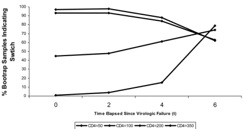
We aimed to identify the origin-specific statically optimal rule for deciding when to modify treatment, given a specific set of covariates ¯S(t). In other words, we estimated for each time point the future switch time expected to maximize CD4 T cell count 8 months later, given covariate values, among individuals who had not yet modified treatment. Following, at each time point, the first action (switch or not) of this optimal treatment plan provided an individualized treatment rule. The static optimality of the rule was origin-specific because it identified, for each time point, the optimal future switch time given that subjects had followed the statically optimal rule itself up till that time point.
Specifically, we considered treatment rules based on current CD4 T cell count and an indicator of viral re-suppression prior to switching regimens. The later covariate was included because our goal was to identify rules for switching among individuals who were infected with resistant HIV. Individuals who achieved viral re-suppression without switching regimens almost certainly did not initially lose suppression due to the presence of resistant virus. Thus,
¯
S(t) = (CD4(t), Sup(t)) where CD4(t) denoted CD4 T-cell count at time t, andSup(t) denoted an indicator that re-suppression of the virus had occurred by timet.
As demonstrated in Lemma 1, the origin-specific statically optimal treat-ment rule for deciding when to switch (among individuals who have not already switched, i.e. ¯a(t−1) = 1) is identified by the parameter
θ(t, a(t)|¯a(t−1) = 1, Sup¯a(t) = 0, CD4¯a(t))
=E(Y¯a(t−1)=1,a(t)(t+ 8)|Sup¯a(t) = 0, CD4¯a(t)).
We further note that, as the outcome is measured at time t + 8, the counterfactuals of interest are in fact indexed only by treatment up till time
t∗ = t + 8− 1 (Y
¯
a(t−1)a(t) = Y¯a(t−1)a(t,t∗)), where we remind the reader that
6.3
Model for counterfactual history-adjusted mean.
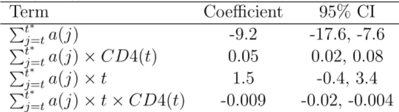
We assumed the following model on the parameterθ(t, a(t, t∗)|a¯(t−1),s¯(t)) =
mβ(t, a(t, t∗)|a¯(t−1)¯s(t)), where mβ(t, a(t, t∗)|¯a(t−1) = 1, Sup(t) = 0, CD4(t)) = β0+β1 t∗ X j=t a(j) +β2CD4(t) +β3t+β4 t∗ X j=t a(j)×CD4(t) +β5 t∗ X j=t a(j)×t+ β6CD4(t)×t+β7 t∗ X j=t a(j)×CD4(t)×t, where Pt∗
j=ta(j) is the residual amount of time until either treatment is
mod-ified or the outcome is measured, under treatment regimen a(t, t∗).
6.4
Model for observed data.
Treatment mechanism. As defined in Subsection 2.1, we assumed sequen-tial randomization; in other words, we assumed that the decision whether to switch treatment or not at each time point only depended on covariates measured prior to that time point. In addition, as defined in Subsection 2.6, we assumed experimental treatment assignment; namely that an individual who had not already switched had some positive probability of both switching treatment and not switching, regardless of her observed past.
Censoring mechanism. We assumed that the probability of being censored at every time point, given that censoring had not already occurred, only de-pended on the observed past (censoring at random):
g( ¯C(T) = 0|O∗)≡ YT t=0 P r(C > t|C¯(t−1) = 0, O∗) = T Y t=0 P r(C1 > t|C¯(t−1) = 0,A¯(t−1),L¯(t−1)) T Y t=0 P r(C2 > t|C1 > t,C¯(t−1) = 0,A¯(t−1),L¯(t−1))
We also made two additional identifiability assumptions (counterpart to the experimental treatment assignment assumption). For each type of censoring and every time point, we assumed that, given that censoring had not already occurred, an individual had some positive probability of not being censored regardless of his observed past: