This is the author’s version of a work that was submitted/accepted for
pub-lication in the following source:
Alonso-Caneiro, David
,
Read, Scott A.
, &
Collins, Michael J.
(2013)
Auto-matic segmentation of choroidal thickness in optical coherence
tomogra-phy.
Biomedical Optics Express
,
4
(12), pp. 2795-2812.
This file was downloaded from:
http://eprints.qut.edu.au/64252/
Notice:
Changes introduced as a result of publishing processes such as
copy-editing and formatting may not be reflected in this document. For a
definitive version of this work, please refer to the published source:
Automatic segmentation of choroidal thickness
in optical coherence tomography
David Alonso-Caneiro, Scott A. Read, and Michael J. Collins
1Contact Lens and Visual Optics Laboratory, School of Optometry and Vision Science, Queensland University of
Technology, Brisbane, Queensland, Australia *[email protected]
Abstract: The assessment of choroidal thickness from optical coherence
tomography (OCT) images of the human choroid is an important clinical and research task, since it provides valuable information regarding the eye’s normal anatomy and physiology, and changes associated with various eye diseases and the development of refractive error. Due to the time consuming and subjective nature of manual image analysis, there is a need for the development of reliable objective automated methods of image segmentation to derive choroidal thickness measures. However, the detection of the two boundaries which delineate the choroid is a complicated and challenging task, in particular the detection of the outer choroidal boundary, due to a number of issues including: (i) the vascular ocular tissue is non-uniform and rich in non-homogeneous features, and (ii) the boundary can have a low contrast. In this paper, an automatic segmentation technique based on graph-search theory is presented to segment the inner choroidal boundary (ICB) and the outer choroidal boundary (OCB) to obtain the choroid thickness profile from OCT images. Before the segmentation, the B-scan is pre-processed to enhance the two boundaries of interest and to minimize the artifacts produced by surrounding features. The algorithm to detect the ICB is based on a simple edge filter and a directional weighted map penalty, while the algorithm to detect the OCB is based on OCT image enhancement and a dual brightness probability gradient. The method was tested on a large data set of images from a pediatric (1083 B-scans) and an adult (90 B-scans) population, which were previously manually segmented by an experienced observer. The results demonstrate the proposed method provides robust detection of the boundaries of interest and is a useful tool to extract clinical data.
2013 Optical Society of America
OCIS codes: (100.0100) Image processing; (100.2960) Image analysis; (110.4500) Optical coherence tomography; (170.4470) Ophthalmology.
References and links
1. D. L. Nickla and J. Wallman, "The multifunctional choroid," Prog Retin Eye Res 29, 144-168 (2010). 2. A. Bill, G. Sperber, and K. Ujiie, "Physiology of the choroidal vascular bed," Int Ophthalmol 6, 101-107
(1983).
3. L. M. Parver, "Temperature modulating action of choroidal blood flow," Eye 5, 181-185 (1991).
4. A. Alm and S. F. Nilsson, "Uveoscleral outflow–a review," Exp Eye Res 88, 760-768 (2009).
5. D. Van Norren and L. Tiemeijer, "Spectral reflectance of the human eye," Vision research 26, 313-320
(1986).
6. S. A. Read, M. J. Collins, S. J. Vincent, and D. Alonso-Caneiro, "Choroidal thickness in childhood," Invest Ophth Vis Sci 54, 3586-3593 (2013).
7. R. Margolis and R. F. Spaide, "A pilot study of enhanced depth imaging optical coherence tomography of the choroid in normal eyes," Am J Ophthalmol 147, 811-815 (2009).
8. M. Esmaeelpour, B. Považay, B. Hermann, B. Hofer, V. Kajic, K. Kapoor, N. J. Sheen, R. V. North, and W. Drexler, "Three-dimensional 1060-nm OCT: choroidal thickness maps in normal subjects and improved posterior segment visualization in cataract patients," Invest Ophth Vis Sci 51, 5260-5266 (2010).
9. V. Manjunath, M. Taha, J. G. Fujimoto, and J. S. Duker, "Choroidal thickness in normal eyes measured using Cirrus HD optical coherence tomography," Am J Ophthalmol 150, 325-329 (2010).
10. M. Hirata, A. Tsujikawa, A. Matsumoto, M. Hangai, S. Ooto, K. Yamashiro, M. Akiba, and N. Yoshimura, "Macular choroidal thickness and volume in normal subjects measured by swept-source optical coherence tomography," Invest Ophth Vis Sci 52, 4971-4978 (2011).
11. X. Q. Li, M. Larsen, and I. C. Munch, "Subfoveal choroidal thickness in relation to sex and axial length in 93 Danish university students," Invest Ophth Vis Sci 52, 8438-8441 (2011).
12. D. S. Dhoot, S. Huo, A. Yuan, D. Xu, S. Srivistava, J. P. Ehlers, E. Traboulsi, and P. K. Kaiser, "Evaluation of choroidal thickness in retinitis pigmentosa using enhanced depth imaging optical coherence tomography," Brit J Ophthalmol 97, 66-69 (2013).
13. Y. Imamura, T. Fujiwara, R. Margolis, and R. F. Spaide, "Enhanced depth imaging optical coherence tomography of the choroid in central serous chorioretinopathy," Retina 29, 1469-1473 (2009).
14. V. Manjunath, J. Goren, J. G. Fujimoto, and J. S. Duker, "Analysis of choroidal thickness in age-related macular degeneration using spectral-domain optical coherence tomography," Am J Ophthalmol 152, 663-668
(2011).
15. M. Esmaeelpour, B. Považay, B. Hermann, B. Hofer, V. Kajic, S. L. Hale, R. V. North, W. Drexler, and N. J. Sheen, "Mapping choroidal and retinal thickness variation in type 2 diabetes using three-dimensional 1060-nm optical coherence tomography," Invest Ophth Vis Sci 52, 5311-5316 (2011).
16. D. A. Sim, P. A. Keane, H. Mehta, S. Fung, J. Zarranz-Ventura, M. Fruttiger, P. J. Patel, C. A. Egan, and A. Tufail, "Repeatability and reproducibility of choroidal vessel layer measurements in diabetic retinopathy using enhanced depth optical coherence tomography," Invest Ophth Vis Sci 54, 2893-2901 (2013).
17. D. Huang, E. A. Swanson, C. P. Lin, J. S. Schuman, W. G. Stinson, W. Chang, M. R. Hee, T. Flotte, K. Gregory, and C. A. Puliafito, "Optical coherence tomography," Science 254, 1178-1181 (1991).
18. M. Wojtkowski, B. Kaluzny, and R. J. Zawadzki, "New directions in ophthalmic optical coherence tomography," Optometry Vision Sci 89, 524-542 (2012).
19. M. Wojtkowski, R. Leitgeb, A. Kowalczyk, T. Bajraszewski, and A. F. Fercher, "In vivo human retinal imaging by Fourier domain optical coherence tomography," J Biomed Opt 7, 457-463 (2002).
20. R. F. Spaide, H. Koizumi, and M. C. Pozonni, "Enhanced depth imaging spectral-domain optical coherence tomography," Am J Ophthalmol 146, 496-500 (2008).
21. B. Považay, K. Bizheva, B. Hermann, A. Unterhuber, H. Sattmann, A. Fercher, W. Drexler, C. Schubert, P. Ahnelt, and M. Mei, "Enhanced visualization of choroidal vessels using ultrahigh resolution ophthalmic OCT at 1050 nm," Opt. Express 11, 1980-1986 (2003).
22. A. Unterhuber, B. Povazay, B. Hermann, H. Sattmann, A. Chavez-Pirson, and W. Drexler, "In vivo retinal optical coherence tomography at 1040 nm-enhanced penetration into the choroid," Opt. Express 13, 3252-3258 (2005).
23. E. C. Lee, J. F. de Boer, M. Mujat, H. Lim, and S. H. Yun, "In vivo optical frequency domain imaging of human retina and choroid," Opt. Express 14, 4403-4411 (2006).
24. Y. Yasuno, Y. Hong, S. Makita, M. Yamanari, M. Akiba, M. Miura, and T. Yatagai, "In vivo high-contrast imaging of deep posterior eye by 1-um swept source optical coherence tomography and scattering optical coherence angiography," Opt. Express 15, 6121-6139 (2007).
25. L. Duan, M. Yamanari, and Y. Yasuno, "Automated phase retardation oriented segmentation of chorio-scleral interface by polarization sensitive optical coherence tomography," Opt. Express 20, 3353-3366
(2012).
26. T. Torzicky, M. Pircher, S. Zotter, M. Bonesi, E. Götzinger, and C. K. Hitzenberger, "Automated measurement of choroidal thickness in the human eye by polarization sensitive optical coherence tomography," Opt. Express 20, 7564-7574 (2012).
27. F. Jaillon, S. Makita, and Y. Yasuno, "Variable velocity range imaging of the choroid with dual-beam optical coherence angiography," Opt. Express 20, 385-396 (2012).
28. B. Braaf, K. A. Vermeer, K. V. Vienola, and J. F. de Boer, "Angiography of the retina and the choroid with phase-resolved OCT using interval-optimized backstitched B-scans," Opt. Express 20, 20516-20534 (2012). 29. H. Ishikawa, D. M. Stein, G. Wollstein, S. Beaton, J. G. Fujimoto, and J. S. Schuman, "Macular
segmentation with optical coherence tomography," Invest Ophth Vis Sci 46, 2012-2017 (2005).
30. T. Fabritius, S. Makita, M. Miura, R. Myllylä, and Y. Yasuno, "Automated segmentation of the macula by optical coherence tomography," Opt. Express 17, 15659-15669 (2009).
31. D. Cabrera Fernández, H. M. Salinas, and C. A. Puliafito, "Automated detection of retinal layer structures on optical coherence tomography images," Opt. Express 13, 10200-10216 (2005).
32. A. Yazdanpanah, G. Hamarneh, B. R. Smith, and M. V. Sarunic, "Segmentation of intra-retinal layers from optical coherence tomography images using an active contour approach," IEEE T Med Imaging 30, 484-496 (2011).
33. A. Mishra, A. Wong, K. Bizheva, and D. A. Clausi, "Intra-retinal layer segmentation in optical coherence tomography images," Opt. Express 17, 23719-23728 (2009).
34. K. Vermeer, J. Van der Schoot, H. Lemij, and J. De Boer, "Automated segmentation by pixel classification of retinal layers in ophthalmic OCT images," Biomed. Opt. Express 2, 1743-1756 (2011).
35. A. Lang, A. Carass, M. Hauser, E. S. Sotirchos, P. A. Calabresi, H. S. Ying, and J. L. Prince, "Retinal layer segmentation of macular OCT images using boundary classification," Biomed. Opt. Express 4, 1133-1152
36. V. Kajić, B. Považay, B. Hermann, B. Hofer, D. Marshall, P. L. Rosin, and W. Drexler, "Robust segmentation of intraretinal layers in the normal human fovea using a novel statistical model based on texture and shape analysis," Opt. Express 18, 14730-14744 (2010).
37. D. Koozekanani, K. Boyer, and C. Roberts, "Retinal thickness measurements from optical coherence tomography using a Markov boundary model," IEEE T Med Imaging 20, 900-916 (2001).
38. S. J. Chiu, X. T. Li, P. Nicholas, C. A. Toth, J. A. Izatt, and S. Farsiu, "Automatic segmentation of seven retinal layers in SDOCT images congruent with expert manual segmentation," Opt. Express 18, 19413 (2010).
39. E. W. Dijkstra, "A note on two problems in connexion with graphs," Numerische mathematik 1, 269-271 (1959).
40. F. LaRocca, S. J. Chiu, R. P. McNabb, A. N. Kuo, J. A. Izatt, and S. Farsiu, "Robust automatic segmentation of corneal layer boundaries in SDOCT images using graph theory and dynamic programming," Biomed. Opt. Express 2, 1524-1538 (2011).
41. Q. Yang, C. A. Reisman, Z. Wang, Y. Fukuma, M. Hangai, N. Yoshimura, A. Tomidokoro, M. Araie, A. S. Raza, and D. C. Hood, "Automated layer segmentation of macular OCT images using dual-scale gradient information," Opt. Express 18, 21293-21307 (2010).
42. M. K. Garvin, M. D. Abràmoff, X. Wu, S. R. Russell, T. L. Burns, and M. Sonka, "Automated 3-D intraretinal layer segmentation of macular spectral-domain optical coherence tomography images," IEEE T Med Imaging 28, 1436-1447 (2009).
43. B. J. Antony, M. D. Abràmoff, M. Sonka, Y. H. Kwon, and M. K. Garvin, "Incorporation of texture-based features in optimal graph-theoretic approach with application to the 3D segmentation of intraretinal surfaces in SD-OCT volumes," in SPIE Medical Imaging, (International Society for Optics and Photonics, 2012), 83141G-83141G-83111.
44. P. Dufour, L. Ceklic, H. Abdillahi, S. Schroder, S. De Zanet, U. Wolf-Schnurrbusch, and J. Kowal, "Graph-based multi-surface segmentation of OCT data using trained hard and soft constraints," IEEE T Med Imaging
32, 531 - 543 (2012).
45. M. Haeker, M. Sonka, R. Kardon, V. A. Shah, X. Wu, and M. D. Abràmoff, "Automated segmentation of intraretinal layers from macular optical coherence tomography images," in Medical Imaging, (International Society for Optics and Photonics, 2007), 651214-651214-651211.
46. K. Lee, M. Niemeijer, M. K. Garvin, Y. H. Kwon, M. Sonka, and M. D. Abràmoff, "Segmentation of the optic disc in 3-D OCT scans of the optic nerve head," IEEE T Med Imaging 29, 159-168 (2010).
47. V. Kajić, M. Esmaeelpour, B. Považay, D. Marshall, P. L. Rosin, and W. Drexler, "Automated choroidal segmentation of 1060 nm OCT in healthy and pathologic eyes using a statistical model," Biomed. Opt. Express 3, 86-103 (2012).
48. L. Zhang, K. Lee, M. Niemeijer, R. F. Mullins, M. Sonka, and M. D. Abràmoff, "Automated segmentation of the choroid from clinical SD-OCT," Invest Ophth Vis Sci 53, 7510-7519 (2012).
49. Z. Hu, X. Wu, Y. Ouyang, Y. Ouyang, and S. R. Sadda, "Semiautomated segmentation of the choroid in spectral-domain optical coherence tomography volume scans," Invest Ophth Vis Sci 54, 1722-1729 (2013).
50. J. Tian, P. Marziliano, M. Baskaran, T. A. Tun, and T. Aung, "Automatic segmentation of the choroid in enhanced depth imaging optical coherence tomography images," Biomed. Opt. Express 4, 397-411 (2013).
51. S. Lee, N. Fallah, F. Forooghian, A. Ko, K. Pakzad-Vaezi, A. B. Merkur, A. W. Kirker, D. A. Albiani, M. Young, and M. V. Sarunic, "Comparative analysis of repeatability of manual and automated choroidal thickness measurements in nonneovascular age-related macular degeneration," Invest Ophth Vis Sci 54, 2864-2871 (2013).
52. K. Li, X. Wu, D. Z. Chen, and M. Sonka, "Optimal surface segmentation in volumetric images-a graph-theoretic approach," IEEE T Pattern Anal 28, 119-134 (2006).
53. S. A. Read, M. J. Collins, S. J. Vincent, and D. Alonso-Caneiro, "Choroidal thickness in myopic and non-myopic children assessed with enhanced depth imaging optical coherence tomography," Invest Ophth Vis Sci, in press (accepted 21/10/2013).
54. S. A. Read, M. J. Collins, S. J. Vincent, and D. Alonso-Caneiro, "Macular retinal layer thickness in childhood," Retina submitted (2013).
55. M. J. Girard, N. G. Strouthidis, C. R. Ethier, and J. M. Mari, "Shadow removal and contrast enhancement in optical coherence tomography images of the human optic nerve head," Invest Ophth Vis Sci 52, 7738-7748
(2011).
56. J. M. Mari, N. G. Strouthidis, S. C. Park, and M. J. Girard, "Enhancement of lamina cribrosa visibility in optical coherence tomography images using adaptive compensation," Invest Ophth Vis Sci 54, 2238-2247
(2013).
57. P. Arbelaez, M. Maire, C. Fowlkes, and J. Malik, "Contour detection and hierarchical image segmentation," IEEE T Pattern Anal 33, 898-916 (2011).
58. D. R. Martin, C. C. Fowlkes, and J. Malik, " Learning to detect natural image boundaries using local brightness, color, and texture cues," IEEE T Pattern Anal 26, 530-549 (2004).
59. J. Canny, "A computational approach to edge detection," IEEE T Pattern Anal, 679-698 (1986).
60. W. Rahman, F. K. Chen, J. Yeoh, P. Patel, A. Tufail, and L. Da Cruz, "Repeatability of manual subfoveal choroidal thickness measurements in healthy subjects using the technique of enhanced depth imaging optical coherence tomography," Invest Ophth Vis Sci 52, 2267-2271 (2011).
1. Introduction
The choroid is the vascular tissue located at the posterior part of the eye between the retina and the sclera. It plays vital physiological roles in the eye [1] including supplying of oxygen and nutrients to the outer retina [2], the regulation of ocular temperature [3] and intraocular pressure [4] and the absorption of light [5]. Studies of healthy eyes have documented variations in choroidal thickness with age in children [6] and in adults [7-9] as well as with increased levels of myopia (i.e. longer axial length) [10, 11]. Additionally, a variety of different eye diseases including retinitis pigmentosa [12], central serous chorioretinopathy [13], age related macular degeneration [14], and diabetic retinopathy [15, 16] have been found to be associated with changes in the thickness of the choroid. Therefore it is important to accurately map the thickness of this vascular layer to understand the natural processes and development of the eye as well as to potentially detect and monitor eye disease.
Since its first introduction in 1991, optical coherence tomography (OCT)[17] has become the standard clinical and research tool for the non-invasive cross-sectional imaging of the posterior eye [18]. Early studies with this technique focused on the quantification of retinal characteristics [19], however recent advances in imaging techniques (i.e. real-time tracking of the eye, averaging of multiple B-scans and enhanced depth imaging (EDI) acquisition) have enabled the capture of high quality images of deeper tissues such as the choroid [7, 20]. In addition to these improvements in many of the clinical OCT instruments, a number of laboratory-based methods have been shown to further enhance the visualization of the choroid including longer wavelength light sources [21-24], the use of polarization sensitive OCT information [25, 26] and choroidal vessel angiography through a Doppler OCT system [27, 28].
Along with the development of the instrumentation, a large body of work has also explored the automatic segmentation of OCT images. Much of the early research focused on the detection of the retinal layers with a range of different image processing techniques. Although the appearance and features of the boundaries between the retinal layers and the choroid layer are different, some of these methods have informed the task of the segmentation of the choroid, therefore a brief review of retinal segmentation methods is included here. A variety of approaches have been used for this task including the segmentation of five layers of the retina based on the intensity, with a pre-processing mean filter to remove speckle [29]. The pixel intensity variations have been used to calculated the total retinal thickness, which involves the segmentation of the inner limiting membrane (ILM) and the retinal pigment epithelium (RPE) layers [30]. A texture analysis by means of the structure tensor combined with complex diffusion filtering was used to segment multiple retinal layers from the B-scans [31]. Additionally, an active contour approach has been adapted for retinal layer segmentation [32], while other studies extended the traditional active contour method with a two-step kernel-based optimization scheme [33]. Other researchers have used more complex imaging segmentation approaches, including support vector machines [34] with features based on image intensities and gradients, random forest classifier [35], texture and shape analysis [36] and Markov boundary models [37].
Graph-search segmentation techniques, which are used in this work, have also been applied in a range of studies to detect the retinal layers. Chiu et al. [38] applied a graph-search segmentation approach using dynamic programming [39] to segment seven retinal layers, which was later extended for segmentation of anterior eye images [40]. Using a similar method Yang et al. [41] utilized a more complex approach to calculate the weights map of the graph-based method, using dual-scale gradient information. Garvin et al. [42] proposed a graph-search approach using multi-surface data (volumetric), which was later extended to incorporate texture based features [43] and hard/soft constraints [44]. Haeker et al. utilized radial scans to generate a composite 3-D image and performed a 3-D graph search of the retinal layers [45], and Lee used multi-scale 3-D graph search for segmenting the optic nerve head [46].
In contrast to the problem of retinal segmentation, the automatic detection of the choroidal layer has not been investigated in as much depth, however a small number of methods have recently been reported. Kajic et al. [47] devised a two stage elaborated statistical model to automatically detect the choroidal boundaries in 1060 nm OCT images, and the algorithm was tested on a range of healthy and pathological eyes. Zhang et al. [48] presented an automated choroidal vasculature segmentation method for the analysis of choroidal vessels with images from a clinical SD-OCT, however the focus of their work was to quantify the vasculature rather than the choroidal thickness. A graph-based approach was used by Hu and colleagues [49] to semi-automatically identify the choroid. Tian et al. [50] also used a graph-search method to segment the choroid in a fully automatic manner, with the weights map created by calculating the local minima of each A-scan in order to obtain a so called valley-pixel, and the graph-search was used to track the valley-pixel that belongs to the choroid boundary by excluding the other surrounding features. Lee et al. [51] adopted previously developed three dimensional graph-cut algorithms, which were initially tested on retinal layers [52], to automatically segment the two layers of interest. Although previous studies of automated choroidal segmentation have reported reasonable agreement between automated analysis and manual segmentation, the detection of the choroidal boundaries in images where the choroidal boundaries are of low contrast (often in cases of thicker choroids) has been reported to be particularly challenging, and may result in large discrepancies between automated and manual results [51].
The vast majority of studies examining choroidal thickness with OCT instruments have utilized manual segmentation methods [6-16], which require subjective judgments and can be time consuming, and potentially prone to bias. Given the small number of methods in the literature for fully automated segmentation of the choroid, this study presents a method to reliably segment the choroidal thickness in OCT images from a clinically available spectral-domain OCT instrument. The proposed routines were tested on a large data set of images from a study with a pediatric population with normal ocular health [53] as well as a set of images from an adult population, which have been previously segmented by an experienced observer. Our proposed method uses graph-search theory techniques and, given the potential challenges in the reliable segmentation of the choroid particularly in cases where the choroidal boundaries are of low contrast, applies novel image enhancement to the choroidal boundaries in order to optimize the segmentation of the choroid.
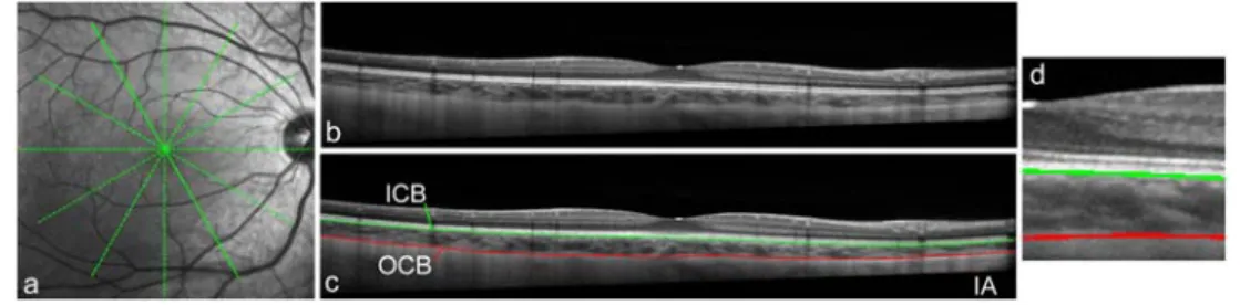
We define the choroidal thickness between the inner choroidal boundary (ICB) and the outer choroidal boundary (OCB), where the ICB coincides with the lower boundary of the retinal pigment epithelium/Bruch’s membrane complex and the OCB marks the transition between choroid and sclera. Fig. 1 shows a typical recording from the data set, including the retinal fundus image to illustrate the location of the scans (Fig. 1(a)) and one selected B-scan (Fig. 1(b)). Additionally the two layers of interest (ICB, OCB) are marked in the figure (Fig. 1(c) and Fig. 1(d)).
The organization of the paper is as follows; Section 2 presents the instrument, dataset and the algorithm used to automatically segment choroidal thickness. Section 3 compares the performance of the automated technique versus the manual segmentation by an experienced observer and examines the detailed performance in a number of example cases, while concluding remarks are given in Section 4.
Fig. 1. Example of the retinal fundus en face image showing the scanning protocol (a) and the spectral domain OCT B-scan captured using the instrument’s high resolution scanning protocol (b). The two layers to be detected are the inner choroidal boundary (ICB-green) and the outer choroidal boundary (OCB-red), where the ICB coincides with the
lower boundary of the retinal pigment epithelium/Bruch’s membrane complex and the OCB marks the transition between choroid and sclera (c). For completeness, an image artifact (IA) sometimes observed during acquisition is
shown. (d) the foveal center is magnified to better appreciate the location of the layers.
2. Materials and methods
2.1. Retrospective data
The retrospective data set used to test the proposed routines contains spectral domain OCT images from one hundred and four children aged between 10 and 15 years of age. Each child had spectral domain OCT chorio-retinal images of their right eye captured using the commercially available Heidelberg Spectralis instrument (Heidelberg Engineering, Heidelberg, Germany). For OCT imaging, the Heidelberg Spectralis uses a super luminescent diode of central wavelength 870 nm, which provides an axial resolution of 3.9 µm and transversal resolution of 14 µm, with a scanning speed of 40,000 A-scans per second. For each participating child, the instrument’s “star” scanning protocol was used to capture 2 series of 6 radial OCT scan lines each separated by 30° and centered on the fovea using the instrument’s enhanced depth imaging (EDI) mode. EDI enhances the visibility of the choroid by focusing the instrument closer to the posterior part of the eye than the standard imaging mode [20]. Additionally, the instrument utilizes a confocal scanning laser ophthalmoscope to automatically track the eye in real-time, and this function was active during the examination to achieve an average of 30 B-scans per each radial OCT image. Each B-scan is 30° long (approximately 8.6 mm, dependent upon each subject’s ocular biometry) and captured using the instrument’s high resolution scanning protocol (each image consists of 496 by 1536 pixels). A small number of children were unable to maintain stable fixation for long enough and so a complete series of 12 radial B-scans was not available for all subjects. For another 8 subjects the complete set of 12 B-scan images could not be analyzed due to the image quality or artifacts, resulting in a final data set of 1083 B-scans available for analysis. To examine the performance of the proposed algorithm on images from subjects of different ages, and to ensure the results are not restricted to the specific age range of the pediatric sample, a second set of images (90 B-scans) from a healthy adult population was also tested. The age of the 15 adult subjects ranged from 18 to 49 years, and the scans were collected using the same imaging protocol as the pediatric sample (1 series of 6 radial line scans were collected per adult subject). A representative set of B-scans, including a range of different healthy subjects and ages, was used during the algorithm’s development.
2.2. Overview of graph-based theory
Unlike the healthy retinal layers, which present a relatively uniform boundary and contrast between adjacent layers, the detection of the OCB is a particular challenge due to a number of features: (i) the depth of the tissue, thus the distance that the light has to travel, means that in many cases the signal reflected off the deeper structures may be relatively weak, making visualization of the OCB difficult, (ii) the vascular nature of the tissue makes the area rich in
features (i.e. vessels) and heterogeneous in structure, which can be difficult to discriminate from the actual choroid-sclera boundary (i.e., the OCB), and (iii) the shape of the choroid also presents greater thickness variations and asymmetries [6] than the retinal layers [54]. We have addressed these detection problems using a graph-theory approach, similar to that proposed by Chiu et al. [38] to segment the retinal layers in OCT images. However, a different strategy was used for the calculation of the weighted maps to segment the ICB and OCB to suit the specific choroidal boundary. For the OCB, first the region is enhanced to compensate for the image intensity attenuation and then a dual brightness gradient is used to populate the weighted map. Tian et al. also applied a graph-based approach [50] to detect the choroid, in which the graph searches thru a number of valley-pixels to detect the smooth choroidal-scleral interface. Their valley-pixels (i.e., local minima of A-scans) are associated with multiple image features in different parts of the image, not only the specific boundary of interest. Thus in their implementation a more sophisticated method of graph search with searching-constraints was implemented. In the algorithm used here, a more sophisticated graph-based weighted map construction is proposed, which uniquely highlights the boundary of interest thus the graph-search does not need to be altered.
Since graph-search theory is the core method used in this work, a brief summary is provided here for completeness, while further details can be found in [38, 39]. The OCT image (B-scan) represents a graph of nodes, where each pixel corresponds to a node. The link between two adjacent nodes is given by a weight value. Dijkstra’s algorithm determines the preferred path between any two nodes on the entire graph by calculating the lowest weight between them. Thus, a start-node and end-node need to be defined. By initializing the nodes at each side of the B-scan, the detected path matches with the layer of interest given the appropriate weight map. To aid the graph to follow the preferred path (i.e. the boundary in the OCT image) and taking into consideration that Dijkstra’s algorithm favors minimum-weighted paths, an additional column of nodes is added to both sides of the image with minimal weights (wmin). This allows an arbitrary assignment of the start and the end nodes at
each side of the B-scan, since the cut will move freely along these columns. After segmentation these two additional columns can be removed. The weight assigned to the edges connecting adjacent nodes a and b is calculated as follow;
min
2 (
)
ab a b
W
g
g
w
(1)Where ga, gb are the gradient information at node a and b respectively with ga, gb∈ [0; 1] and
wmin is the minimum weight in the graph, set to a constant value of 10-5. In here a 4-nodes
connection is assumed, thus each node (i.e., pixel) is connected with four adjacent nodes (right, top, left, and bottom), for the proposed technique this connection scheme was found to provide a more robust performance and was less influenced by the surrounding choroidal vasculature than an 8-nodes connection. After the weights maps are calculated, Dijkstra's algorithm [39] is used to determine the lowest weighted path of a graph between the start and end nodes. The resulting path marks the boundary of interest in the B-scan.
Therefore, since the weighted map (calculated from the gradient information) determines the path to be segmented, the method of determining the map should highlight the layer of interest (OCB or ICB) while suppressing the surrounding information. In this study, two different methods are applied to the ICB and OCB, respectively. The algorithm to detect ICB is based on a simple edge filter and a directional weight map penalty, while the algorithm to detect OCB is based on OCT image enhancement and dual brightness probability gradient. Each of the steps involved in the algorithm is detailed in the following subsections.
Next we define the OCT image (B-scan) as I(i, j), where I is the pixel intensity value for a pixel located in the i-th row and the j-th column, with i ∈ [1; p] and j ∈ [1; q], and where p × q represents the total number of pixels. Following the matrix convention, indexes
I(1,1) indicate the top-left corner of the image. The original image is rescaled using a bicubic interpolation to obtain an aspect ratio 1:1 by rescaling into the highest resolution scale, which results in a B-scan image of equal axial and transversal resolution of 3.9 µm (496 x 2245 pixels). The aspect ratio of the image will have an influence on the segmentation outcome, since it determines the number of nodes of the weighted map and as a consequence the segmented path. Therefore the aspect ratio that is used in the process should be taken into consideration for optimum segmentation results.
During the acquisition of the OCT images, the Heidelberg Spectralis OCT instrument can crop certain regions from the B-scan as a consequence of the B-scan registration and averaging process employed by the instrument. These cropped regions usually appear in the lower region of the B-scan as a dark area (see Fig. 1(c)) and could create an artificial edge that needs to be masked from the final weighted map. This effect may be specific to the instrument used in this study (Heidelberg Spectralis).
2.3. Inner Choroid Boundary (ICB): segmentation
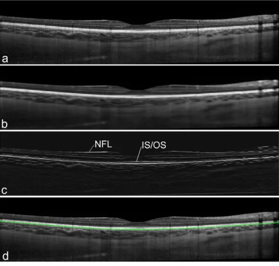
The lower boundary of the retinal pigment epithelium/Bruch’s membrane complex (RPE, see Figure 1) marks the transition between the retina and the choroid, and therefore is the ICB. This layer has extremely hyper-reflective properties, making its detection more straightforward compared to the outer choroidal boundary. Before calculating the weights map, the image intensity was normalized by dividing each A-scan by its maximum intensity value. To further highlight the ICB, pixels with intensity below 75% of the maximum were divided by 0.8. After which, a course average filter was run through the image with a rectangular size of 5 x 22 pixels, to smooth the image. Fig. 2(b) shows an example of the image after the pre-processing.
A simple filter edge map [1;-1], which highlights the bright-to-dark transition in the vertical direction, can be used to detect the ICB and to extract the gradient information used in the calculation of the weighted map. However, the adjacent inner segment/outer segment band (IS/OS) and/or the nerve fibre layer (NFL) (see Figure 2) will also create an edge due to their similar hyper-reflective nature. To minimize the effect from the IS/OS layer, before applying the edge filter, the image columns are resized by half using a bicubic interpolation (i.e. A-scan resize), which reduces the gap between the IS/OS and the RPE layers and thus partly removes the edge information (see Fig. 2(c), image shown at the same scale as original). To prevent the graph path drifting into the adjacent IS/OS or the upper NFL, the resulting gradient information rows are rescaled back into their original dimensions before calculating the weighted map using Eq. 1. Although by rescaling the weighted map there is a sacrifice in computational time due to the increase in path-nodes, the aim of this work was to obtain a reliable ICB segmentation. Therefore, this rescale creates a directional weight penalty in the vertical direction which achieves a more robust detection of the ICB and avoids the path drifting into the IS/OS or NFL. Fig. 2(c) shows the original image with the resulting ICB marked as a green solid line.
Figure 2. Example of the inner choroidal boundary segmentation steps, including the original B-scan (a), the pre-processed image (b), the vertical gradient information shown at the same scale as the original (c) and the original image with the segmented ICB result as a solid green line (d). For completeness the potential edge effect created by
the two retinal layers is marked (IS/OS, NFL).
2.4. Flattening of the image and cropping the choroidal region
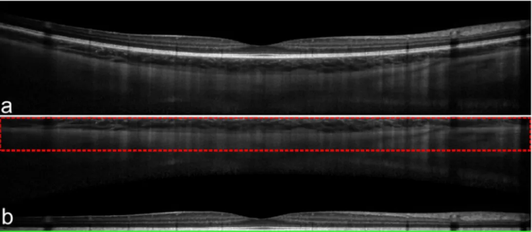
Since Dijkstra's algorithm [39] determines the lowest weighted path from the start to the end nodes, the shortest geometric path could trigger undesirable results since lesser nodes could result in lesser final weight and this effect is particularly significant for the OCB. In order to approximate the shortest geometric path with the minimum weighted path, the image shape can be transformed. Considering that the shape of the back of the eye is approximately spherical, the ICB can be used as a reference to compensate this effect and to flatten the image. Although the actual shape of the retina can vary depending on a number of factors such as the location of the scan, the axial length of the eye and the actual length of the scan, in general, it is safe to assume this spherical shape and to flatten the B-scan [38]. To flatten the image, each A-scan (image column) is circularly shifted to set the ICB boundary in the bottom part of the image, leaving the choroidal section on the top of the B-scan. Fig. 3 shows an example of the B-scan flattening; where the original B-scan Fig. 3(a) is flattened using the ICB estimate, Fig. 3(b). After flattening the image, a rectangular region at the top of the image, which contains the choroid, can be cropped to remove image information that is not relevant to the outer choroidal boundary detection. The height of the region to be cropped was
set to be large enough to encompass a region well above the maximum thickness expected for the population [6], thus setting the area to a thickness of 565 microns. Fig. 3(b), highlights the region of interest with a dashed red box, which is used in the following detection steps.
Figure 3. Original B-scan (a) and its equivalent flattened version (b). The red dotted box represents the cropped region of interest (~565 microns thick), to be used during the OCB segmentation.
2.5. Outer choroid boundary (OCB): image enhancement
The quality of the choroid’s visibility is influenced by a number of factors including, the shadows cast by blood vessels, the depth of the tissue, and limitations of the imaging technique. As a result, the reflected signals from the deeper OCB structure may be too weak to be reliably visualized. Thus, an enhancement of the OCB boundary is required, while minimizing the effect of the surrounding vessels. Girard et al. [55] presented a method, inspired by previous research with ultrasound, to compensate the attenuation of OCT images and to enhance the visibility of the deeper ocular structures at the optic nerve head as well as to remove the shadows cast from vessels. The method was later improved by adding an adaptive compensation step to overcome the over-amplification limitation of the initial algorithm, and the technique was successfully used to enhance the visibility of the OCT image of the human optic nerve head [56].
The compensation algorithm, shown below in Eq. 2, restores the strongly attenuated image and uses an expansion to further provide a contrast enhancement [55]. The intensity-expansion operator (exponentiation) can be used to increase the dynamic range of pixel intensities, which improves the ability of edge detection and segmentation between adjacent tissue layers of low contrast, which is of special interest to detect the OCB. The contrast enhancement method follows the equation:
(i, j)
( , )
2
(i, j)
n raw p n raw k iI
L i j
I
(2)Where p is the maximum number of pixel per A-scan. As discussed in [55], the value of the exponentiation (n) was set to two. Although n values above this could increase contrast further, there seems to be a negative effect due to the increase of speckle noise with higher n values, which could compromise the detection of the OCB. It should be noted that the
processing of the B-scans must be done in raw format (Iraw). Commercial instruments
commonly apply an intensity-compression operation (i.e. logarithmic or nth root) to the raw OCT image, in order to better visualize simultaneously strong and weak signals within a given OCT image. This intensity-compression reduces the dynamic range of pixel intensities. For the Heidelberg Spectralis, the following transformation (define in Eq. 3) is applied to the raw image to better visualize all the structures.
4
(i, j) 255
raw(i, j)
I
I
(3)Thus, to transform the B-scan back into its raw version the following transformation (define in Eq. 4) is applied; 4
(i, j)
( , )
255
rawI
I
i j
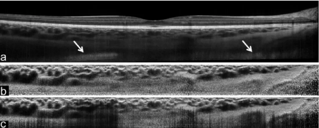
(4)Although the work present by Girard et al. [55] applies the enhancement to the entire B-scan, it was noted during the development of our technique for enhancement of the choroid, that in B-scans with artifacts, such as mirror images (see Fig. 4(a)), the algorithm fails to provide an appropriate enhanced image. Thus, in this study the image enhancement step was applied to the smaller cropped region of interest after the previous flattening step (Fig. 3(b)), rather than to the entire image. Fig. 4 compares the effect of cropping the region of interest first and then applying the image enhancement (Fig. 4(b)) versus enhancing the entire image followed by cropping the region of interest (Fig. 4(c)). In this example, it is easy to observe the undesirable effect that the mirror image artifact can have on the image enhancement.
Fig. 4. Example of the image enhancement of a B-scan with artifacts (mirror image artifact marked by arrows). The proposed method uniquely enhances the region of interest after cropping (b) versus enhancing the whole B-scan and
then extracting the region of interest (c).
After the image enhancement is completed, the image is retained in its raw format. Then, rather than an intensity-compression, the image is adjusted using a predefined intensity range, so that 25% of the data at high intensity is saturated. In other words, data within this upper 25% range is clipped to the maximum upper limit. Figure 5 shows the original image (Fig. 5(a)) and the result of transformation (Fig. 5(b)). To further minimize the effect from the vessels which could influence the subsequent edge detection (specifically the upper
choriocapillaris), a mask is applied to the image. The mask multiplies each row by its row number. Thus following the matrix convention, the upper-most row will be multiplied by 1 and the bottom-most row by J, where J is the maximum pixel number of the cropped region (145 pixels). This mask decreases the intensity of the uppermost choroidal vessels and highlights the scleral tissue, thus delineating the OCB. After this, a course average filter was run through the image with a rectangular size of 2 x 22 pixels to smooth the image, Fig. 5(c).
While calculating the transformation, the contrast enhancement factor (denominator sum in Eq. 2) will eventually become small at deeper positions within the tissue (for values of k close to p, in Eq. 2), which results in abnormally high pixel intensities (an over-amplified area). This can be an issue during the detection process and thus a small portion of the lower part of the image was removed, before the subsequent analysis. Although the original method from Girard et al. [55] was later improved in [56] by including an adaptive compensation, we used a simple cropping to remove the over-amplified area in the image (the bottom 15 rows were removed from the image).
Figure 5. Example of the outer choroidal boundary segmentation steps, including the original cropped region (a), the enhanced and intensity-adjusted transformation (b), the masked and smoothed B-scan (c), individual gradient outputs
2.6 Outer choroid boundary (OCB): weights maps and segmentation
Instead of the simple edge detector used to calculate the gradient information of the inner choroidal boundary, for the outer choroidal boundary a dual gradient probability approach is used. This gradient-based boundary detector is derived from Arbelaez and colleagues [57] work, in which they model the probability of a pixel being on-boundary.
The output of the gradient-based boundary detector is an image that provides the posterior probability of a boundary at each pixel, for the OCT B-scan. Thus, the main component of the probability contour detector is the oriented gradient signal G(i,j,θ) which is defined for an intensity image I(i,j). The gradient features used by [58] to predict probability of a boundary is based on the histogram difference between the two halves of a single disc. The orientation of the dividing disc-diagonal sets the orientation of the gradient, and the radius of the disc sets the scale. Thus to calculate the gradient magnitude at the image location (i,j), we considered a circular disc centered at (i,j) and split by a diameter at an angle θ. The histograms of intensity values in each half-disc are computed and gives as k and h. Then the X2 distance (defined in
Eq. 5) between the two half-disc histograms k and h is calculated to obtain the gradient value:
2 2
( , )
1
(k( ) h( ))
2
sk( ) h(s)
s
s
k h
s
(5)Once the oriented gradient signal G(i,j,θ) is calculated, a filter is applied to enhance local maxima and smooth out multiple detection peaks in the direction orthogonal to θ. Based on [57], this operation is equivalent to fitting a cylindrical parabola, whose axis is orientated along the direction θ, to a local 2D window surrounding each pixel and replacing the response at the pixel with that estimated by the fit. Given the aspect ratio of the image and the flattening of the B-scan, the orientation of the boundary can be assumed to be parallel to the B-scan, thus a single orientation is used (i.e., θ = 0°). The radius of the disk was empirically set to 22 pixels.
Once the brightness gradient G(i,j,0) is calculated a dual gradient-based boundary is extracted. The first component of the gradient is based on the non-maximum suppression [59] in the orientation of interest, which produces thinned, real-valued contours. The non-maximum suppression has the effect of cancelling all image information that is not part of local maxima. Therefore, this first approach provides a very selective (coarse) probability estimator of the boundary (Fig. 5(d)).
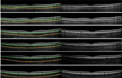
The second component aims to smooth the coarse probability of the first boundary estimator, by multiplying the output of the Canny edge detector of the original image by the brightness gradient G(i,j,0). Matlab’s implementation of Canny’s edge detector, which automatically selects the threshold, was used here. This probability estimator is less selective and therefore helps the graph-search to search for the smooth transition between areas (Fig. 5(e)). Both gradients are averaged to obtain the dual gradient-based probability boundary (Fig. 5(f)). Similar to the ICB, the gradient information is rescaled in the vertical direction by 1.5x times the original value, to avoid the path drifting into any surrounding vessel features. The final result of the OCB segmentation is shown in the Fig. 5(g). Additionally, Fig. 6 shows six other representative results from the segmentation of OCB and ICB, from B-scans from the pediatric and the adult datasets.
Figure 6. Six B-scans from six different subjects are shown with the derived inner and outer choroidal boundaries (left), along with the original B-Scan images (right). The B-scans represent a range of different examples (i.e. with
typical variations in overall choroidal thickness, thickness profiles and choroidal contrast). The images have been arranged in decreasing order in terms of the contrast at the OCB layer. The segmentation based on the manual analysis (yellow) and the automatic analysis (red) for the OCBs is shown as well as the automatic segmentation of the
ICB (green). The manual ICB was not included since it matches closely to the automatic. The first five B-scans are from pediatric subjects and the last B-scans from an adult.
3. Results and discussion
3.1 Automated versus manual segmentation results
To evaluate the performance of the algorithm in the analysis of the images from the pediatric and adult samples, the results from the automatic segmentation of the choroid were compared with the manual segmentation performed by an experienced observer. The observer who performed the manual segmentation of all images was instructed to analyze each scan by segmenting the two boundaries of interest, in order to determine choroidal thickness across the 30° width of each scan. The ICB was an automated segmentation (based on graph-theory [38] as previously presented by the authors [53]) which the observer could manually correct if any segmentation errors occurred. For the OCB, the observer manually selected (an average of 22 points along) the boundary and the software then automatically fit a smooth function (spline fit) to these points to define the boundary.
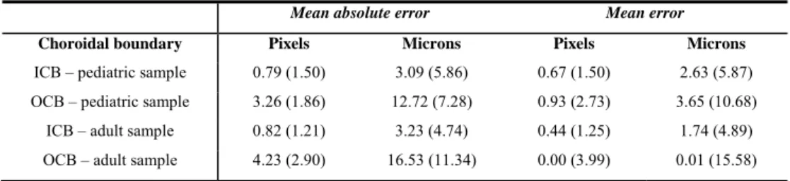
Once the boundaries were computed for each image by both the automatic and manual techniques, the measurement error between the manual and automatic analysis for an entire B-scan can be derived. Two common measurements of error were used here to evaluate the performance of the automatic method, the mean error and the mean absolute error. The mean values of these two error metrics for the 1083 images from the pediatric population and the 90 images from the adult population can be found in Table 1 for the two boundaries of interest. Taking into account that the axial resolution of the OCT is 3.9 microns per pixel, the results are reported in both microns and pixels. Positive errors, in the mean error, indicate that the location of the automatic boundary was above the manual boundary in the image. Overall, the ICB segmentation results present lower mean errors and standard deviation than the OCB. It is worth noting that the mean error for both boundaries is lower than the instrument’s axial resolution.
Regarding the accuracy of the proposed technique, it is not surprising to observe that the segmentation of the ICB performs better than the OCB, due to the hyper-reflective nature of the layer. Out of the 1173 B-scans only 8 (0.7% of the total) had the ICB incorrectly segmented (3 B-scan had IS/OS segmented instead and the other 5 the NFL). Therefore, for this well-defined ICB, the mean absolute error between manual and automatic method is minimal (2.63 microns). This error is comparable with previous studies which have reported the detection of this layer, using different methods such as random forest classifier methods [35] (mean absolute error of 3.50 microns) and another graph-search strategy that obtained a mean absolute error of 2.35 microns for the ICB. The OCB presents greater difficulty for automated segmentation, yet the mean absolute error is still relatively small (12.72 microns for the pediatric and 16.53 for the adults). This result for the OCB is also comparable with a previously reported method of choroidal segmentation using semi-automatic methods [49] that obtained mean absolute errors between 7.21 and 27.23 microns for normal subjects and 25.72 microns for subjects with pathology.
Table 1. Difference in boundary position between the proposed algorithm and the manual observer for the entire pediatric dataset (1083 B-scans) and the adult dataset (90 B-scans). The results are reported in mean values and
(standard deviation) in two units (pixels and microns).
Mean absolute error Mean error
Choroidal boundary Pixels Microns Pixels Microns
ICB – pediatric sample 0.79 (1.50) 3.09 (5.86) 0.67 (1.50) 2.63 (5.87)
OCB – pediatric sample 3.26 (1.86) 12.72 (7.28) 0.93 (2.73) 3.65 (10.68)
ICB – adult sample 0.82 (1.21) 3.23 (4.74) 0.44 (1.25) 1.74 (4.89)
OCB – adult sample 4.23 (2.90) 16.53 (11.34) 0.00 (3.99) 0.01 (15.58)
Up to this point, the focus of the analysis has been on the evaluation of the accuracy of the boundary estimation. However, the clinically important measurement derived from the segmentation of the boundaries is the choroidal thickness. Table 2 shows the mean choroidal thickness difference between the manual and automatic methods for the 1083 images from the pediatric sample and the 90 images from the adult sample included in this study. For comparison, the observer was asked to repeat the manual analysis for 120 B-scans from 20 randomly selected subjects and the observer’s repeatability error (i.e. the first repeat minus the second repeat) is also shown in Table 2. It is worth noting that the mean values for both methods are comparable, however the observer’s repeatability presents slightly lower variability.
The error in the choroidal thickness (Table 2), which is more clinically relevant than the boundary performance, shows a mean absolute error of 12.96 microns (3.32 pixels) in the pediatric subjects and 16.27 microns (4.17 pixels) in the adults. Interestingly, these errors are close to the observer’s repeatability error (8.01 microns and 2.05 pixels). In other words, the average difference between the automatic segmentation and the segmentation of an experienced observer is of similar magnitude to the average difference between two repeated analyses on the same scan by the same observer. Taking into consideration that the observer’s repeatability error is a more conservative measurement than the normally reported between-observer variability, this is a very positive result. For example, Rahman and colleagues showed that for choroidal thickness [60], the intra-observer difference was approximately 23 microns (95% confidence interval, 19–26 microns), whereas inter-observer was greater at 32 (95% CI, 30–34 microns).
To examine if there were regional variations in the algorithm performance, we also determined the error between the manually and automatically derived choroidal thickness values in 4 different spatial regions of the analyzed B-scans (subfoveal, central fovea and the inner and outer macular regions). This analysis did not reveal any obvious regional changes across the B-scans in the mean errors (the mean absolute error ranged from 3.32 to 3.48
pixels, and the mean error from -0.66 to -0.54 pixels across the 4 considered regions), which suggests that the algorithm is performing similarly across the different regions of the B-scan.
Table 2. Difference in choroidal thickness between the proposed algorithm and the manual observer for the entire pediatric dataset (1083 B-scans) and the adult dataset (90 B-scans). The observer repeatability is also given in a
random selected subset of images (120 B-scans).
Absolute mean error Mean error
Pixels Microns Pixels Microns
Choroidal thickness difference
pediatric sample 3.32 (2.30) 12.96 (9.00) -0.26 (3.18) -1.01 (12.43)
Choroidal thickness difference
adult sample 4.17 (2.94) 16.27 (11.48) 0.60 (3.97) 2.35 (15.48)
Observer’s repeatability 2.05 (0.85) 8.01 (3.34) -0.34 (1.56) -1.34 (6.08)
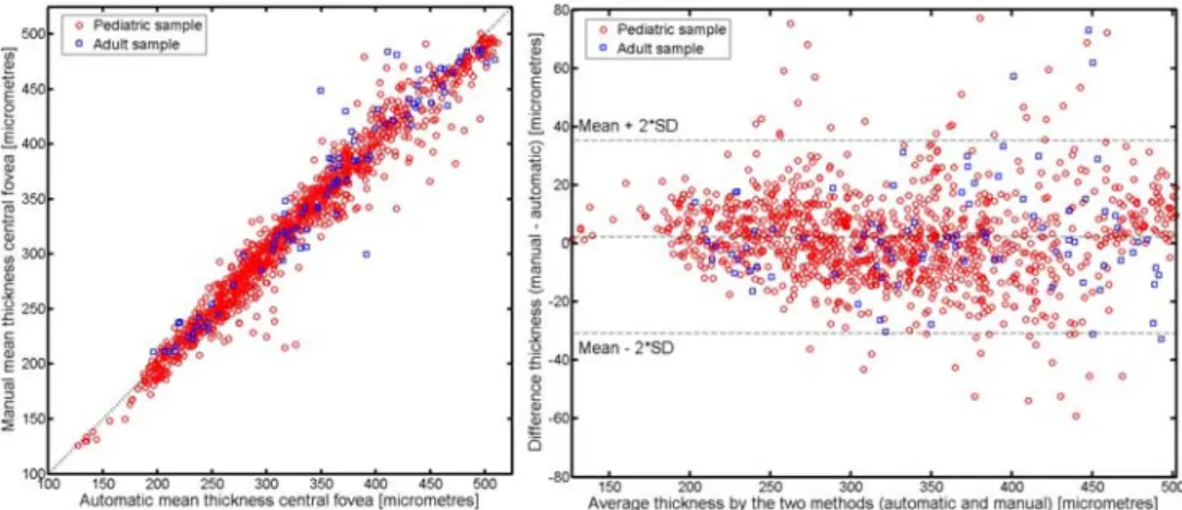
Figure 7 compares the central foveal thickness (calculated as the mean thickness across the central 1 mm of the B-scan) for the automatic and manual methods. The two methods were highly correlated with an r2 of 0.98 and 0.96 for the pediatric and adult sample respectively
(Fig. 7(a)). The Bland-Altman (Fig. 7(b)) plot for the same set of data is also shown and illustrates good agreement between the two methods, and does not appear to exhibit an obvious association between the measurement error and the mean choroidal thickness. For the pediatric sample the mean between method difference was 2.29 ± 16.54 microns (95% confidence intervals 35.37 to -30.79 microns), for the adult sample the mean between method difference was -2.52 ± 23.22 microns (95% confidence intervals 43.92 to -48.98 microns).
Tian et al. [50] examined the performance of their automated choroidal segmentation algorithm using Dice’s coefficient (a measure based upon the proportion of overlapping of the contour area between the manual and automatic analysis), and reported an average coefficient (+-SD) of 90.5% (3%), over their 45 images. To allow a more direct comparison between Tian et al’s method and our current work, we also calculated Dice’s coefficient for our two datasets, and found an average coefficient of 97.3% (1.5%) and 96.7% (2.1%) for the pediatric and adult populations, respectively. However, since Dice’s coefficient relies upon the proportion of area overlapping between the manual and automatic segmentation, the actual thickness of the choroid can skew the results and thus the boundary position difference that we have reported earlier likely provides a more reliable assessment of the algorithm’s performance.
Figure 7. Correlation between the automatic and manual methods for measurements of central choroidal thickness (black dotted line indicates the line of equality between the two measures) (a). Bland–Altman plot of the difference
vs. the mean of the two methods for measurements of central choroidal thickness (b). The red circles represent the pediatric sample and the blue squares the adult sample.
3.2. Other results
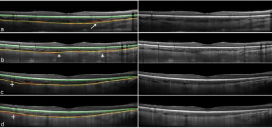
Tables 1 and 2 illustrate the close agreement between the automatic and manual methods. However, it is also important to understand the disagreement. A few examples of interest are discussed here and presented in Fig. 8, with the results from the manual observer (yellow solid line) compared with the automatic method (red dotted line). Taking into account that the manual observer selected an average of 22 points along the boundary and then a smooth spline was fit to the boundary, the observer’s result is in general a smoother version of the automatic boundary. Therefore it is not surprising that blood vessels located close to the OCB can deviate the results of the automatic method as shown in Fig. 8(a). Similarly, the ciliary vessels which run thru the sclera and insert into the choroid can result in a gap in the OCB that alters the boundary position in the automatic analysis (Fig. 8(b)). For these cases, the observer’s expertise appears to provide a more robust result. However, in other cases the intensity changes at the choroidal layer could mislead the observer. For example in Fig. 8 (c) & (d) we present the two repeated B-scans taken on the same subject and location. The intensity change in the left side of Fig. 8(d) appears to lead the observer to pick the wrong boundary, while the automatic method picks the same boundary, which is probably due to the intensity compensation method used during the detection of the OCB.
Figure 8. Example of four B-scans with disagreement between the manual (yellow line) and automatic methods (red line), due to the choroidal vessels (a, arrow), the ciliary vessel travelling through the sclera (b,asterisks) and the changes in intensity in the choroidal boundary (c,d, plus-sign). The last two panels (c,d) correspond to consecutive
scans from the same subject and illustrate how the intensity changes cause a manual segmentation error.
4. Conclusions
A novel approach for the segmentation of the inner and outer choroidal boundaries in OCT images was presented. The method uses graph-search theory to segment the two boundaries of interest, applying two different strategies to calculate the graph weight maps. For the ICB detection, the algorithm uses an edge filter and a directional weight map penalty, while the OCB detection algorithm is based on OCT choroidal image enhancement and dual brightness probability gradient information. This new approach provides accurate results even under low B-scan contrast conditions and also appears to effectively remove choroidal vessel artifacts from the OCB segmentation. From the results obtained on a large pediatric dataset containing 1083 B-scans and an adult dataset containing 90 B-scans, the method shows a close agreement
with manual analysis performed by an experienced observer for the two layers of interest and consequently with the choroidal thickness.
Despite the encouraging results given by the technique in this large data set of images, which allowed the efficacy of the algorithm to be tested across a wide variety of different choroidal morphologies, there are a number of factors that should be considered. All the B-scans had a quality index (QI) value greater than 20 (the mean QI from all measurements was 33 ± 3 dB) as per the manufacturer recommendations. Although the QI provides a measure of the scan’s signal to noise ratio, it is unclear whether this measure reliably reflects the quality of the choroid in the image. However, given that the images shown in Fig. 6 all exhibited a good QI (>20dB), the actual contrast in the OCB boundary does not necessarily reflect the QI of the image. This QI may more closely reflect the image quality of the ICB but not the OCB. It is also acknowledged that none of the subjects from the dataset had retinal or choroidal pathologies. Previous reports have found that the detection of the choroid in subjects with posterior segment pathology is prone to higher detection errors [47, 49]. Increased media opacities with age may also influence OCT image quality and the strength of the choroidal signal in the images [8]. Thus, the use of the proposed method in older adult subjects and in those with posterior segment pathology should be validated in the future.
The current processing time for the algorithm is about 45 seconds per B-scan, using non-optimized implementation. For our application, the computational time was not considered critical since real time processing was not needed as all of the data was processed off-line. Any improvements in the methods were therefore aimed to benefit the boundary segmentation accuracy rather than the computational time. Similarly, the method was designed for single B-scans, however it could be extended to 3-D volumetric graph-approach, in a similar way as reported for retinal segmentation methods [42-44].
It is clear while looking at the B-scans that the manual detection of the choroidal boundaries is a complicated and time consuming task requiring subjective judgments, particularly for the detection of the OCB due to its low contrast and poorly defined boundary features. The method proposed here provides encouraging results for the automated segmentation of optical coherence tomograms of the human choroid from pediatric and adult subjects, with a close agreement with the results from an experienced human observer.
Acknowledgments
Supported by Australian Research Council ‘‘Discovery Early Career Research Award’’ DE120101434 (Scott A. Read). The authors acknowledge the assistance of Rod Jensen in the manual analysis of the OCT images.