University of Wollongong
Research Online
Faculty of Engineering and Information Sciences
-Papers: Part A
Faculty of Engineering and Information Sciences
2015
Video classification based on spatial gradient and
optical flow descriptors
Xiaolin Tang
University of Wollongong, [email protected]
Abdesselam Bouzerdoum
University of Wollongong, [email protected]
Son Lam Phung
University of Wollongong, [email protected]
Research Online is the open access institutional repository for the University of Wollongong. For further information contact the UOW Library: [email protected]
Publication Details
X. Tang, A. Bouzerdoum & S. Lam. Phung, "Video classification based on spatial gradient and optical flow descriptors," in Digital Image Computing: Techniques and Applications (DICTA), 2015 International Conference on, 2015, pp. 1-8.
Video classification based on spatial gradient and optical flow descriptors
Abstract
Feature point detection and local feature extraction are the two critical steps in trajectory-based methods for
video classification. This paper proposes to detect trajectories by tracking the spatiotemporal feature points in
salient regions instead of the entire frame. This strategy significantly reduces noisy feature points in the
background region, and leads to lower computational cost and higher discriminative power of the feature set.
Two new spatiotemporal descriptors, namely the STOH and RISTOH are proposed to describe the
spatiotemporal characteristics of the moving object. The proposed method for feature point detection and
local feature extraction is applied for human action recognition. It is evaluated on three video datasets: KTH,
YouTube, and Hollywood2. The results show that the proposed method achieves a higher classification rate,
even when it uses only half the number of feature points compared to the dense sampling approach. Moreover,
features extracted from the curvature of the motion surface are more discriminative than features extracted
from the spatial gradient.
Keywords
video, classification, spatial, gradient, flow, optical, descriptors
DisciplinesEngineering | Science and Technology Studies
Publication DetailsX. Tang, A. Bouzerdoum & S. Lam. Phung, "Video classification based on spatial gradient and optical flow
descriptors," in Digital Image Computing: Techniques and Applications (DICTA), 2015 International
Conference on, 2015, pp. 1-8.
Video Classification based on Spatial Gradient and
Optical Flow Descriptors
Xiaolin Tang, Abdesselam Bouzerdoum, and Son Lam Phung
School of Electrical, Computer and Telecommunications Engineering University of Wollongong, Australia
E-mail: [email protected], [email protected], [email protected]
Abstract—Feature point detection and local feature extraction
are the two critical steps in trajectory-based methods for video classification. This paper proposes to detect trajectories by tracking the spatiotemporal feature points in salient regions instead of the entire frame. This strategy significantly reduces noisy feature points in the background region, and leads to lower computational cost and higher discriminative power of the feature set. Two new spatiotemporal descriptors, namely the STOH and RISTOH are proposed to describe the spatiotemporal characteristics of the moving object. The proposed method for feature point detection and local feature extraction is applied for human action recognition. It is evaluated on three video datasets: KTH, YouTube, and Hollywood2. The results show that the proposed method achieves a higher classification rate, even when it uses only half the number of feature points compared to the dense sampling approach. Moreover, features extracted from the curvature of the motion surface are more discriminative than features extracted from the spatial gradient.
I. INTRODUCTION
Efficient and reliable video classification is of critical im-portance for several video management tasks, such as video annotation, action recognition, video summarization or violent scene detection. Despite the existing excellent techniques, video classification continues to be one of the most challenging problems in computer vision.
In the human visual system (HVS), the discriminative cues for object and action recognition come from the objects of interest and their surrounding areas, which are known as the salient region. The rest of the observable scene (either static or moving) constitutes the background region, which is meaningless for recognition and is generally ignored [1]. By analogy with the HVS, features used in computer vision should be extracted from the salient region to improve robustness to background variations and, moreover, to obtain a compact and discriminative feature set. The saliency concept is not new in image analysis, and a number of techniques have been developed for salient region detection [2]–[7]. In the past few years, several researchers have extended the salient region detection problem from image to video [1], [8]–[11]. However, there are few video classification algorithms that employ the salient region detection method for feature extraction.
In this paper, we first propose to detect feature points from the spatiotemporal salient region, and then follow the pipeline of the trajectory-based approach [12], which gives rise to the state-of-the-art result in video classification. The spatiotem-poral salient region in the video sequence is calculated by a
graph-based manifold ranking algorithm [6], which ranks the unlabeled nodes based on their relevance to the query nodes. Local spatiotemporal features have recently become popular in trajectory-based action recognition [12]–[14]. Generally, local features are extracted from the spatial gradient, temporal difference, optical flow, and trajectory, which reveals either the spatial structure or temporal motion of the video content. The most distinct spatiotemporal structure of the objects in the video is the motion surface which not only reflects the shape but also records the moving trace. However, it is hard to get the exact moving surface due to the camera motion, illumi-nation changes, low contrast, and sudden and swift motion of the object. Considering the fact that the moving surface, in essence, is the result of edge motion over time, we propose to compute the raw motion surface using a combination of the spatial gradient and optical flow. Furthermore, extensions of the HOG (histogram of oriented gradients) and SIFT (scale invariant feature transform) descriptors are developed based on the curvature of the raw motion surface in small video patches surrounding the feature points.
This paper is organized as follows. Section II describes the related work for video classification. Section III presents the salient feature point detection method, and Section IV introduces the proposed features based on the curvature of moving surface. Section V shows the experiment results and analysis, and Section VI gives the concluding remarks.
II. RELATED WORK
In the past few years, many approaches for video classifi-cation have been developed. Among the approaches that yield state-of-the-art classification results are the feature learning approach [15]–[17] and the trajectory-based approach [12]– [14], [18]. Recently, deep learning has gained popularity, where several feature extraction layers are stacked together. The local features are generally learned by training each convolutional layer separately using convolutional neural net-works (CNN) [16], [19], [20] or independent component analysis (ICA) [17] and its variants [15]. In CNN, each frame is treated as an independent unit for feature extraction, and thus the local features only contain spatial properties; the temporal correlation between successive frames is extracted by a separate network. ICA, on the other hand, is capable of extracting spatiotemporal local features since the basic unit for feature extraction is a video patch. However, ICA cannot
extract complex and non-linear features since itself is a linear projection. Compared with the hand-crafted features, features learned by CNN or ICA are not transparent and have no obvious physical meaning.
In trajectory-based methods, dense point trajectories are calculated based on the dense optical flow [12], [14]. The SIFT point trajectories are, on the other hand, obtained by tracking the SIFT points using feature matching [13], and Harris point trajectories are obtained by tracking Harris points using Kanade-Lucas-Tomasi (KLT) tracker [18], [21]. The feature matching method and KLT tracker enable the extraction of the exact traces of the feature points. However, the two methods can easily be affected by the motion of the object, and thereby the long term trajectories, especially for the moving objects, are sparse. By contrast, the optical flow based tracking method gives coarse feature point traces, but it is able to track every pixel as long as possible, until the feature points disappear from the video. Empirical results indicate that dense and raw trajectory-based approaches outperform the sparse and accurate trajectory-based approaches [14].
In the trajectory-based approaches, hand-crafted features are extracted from a cuboid whose central axis is the trace of the feature point. The most commonly used local features are HOG, HOF, MBH [22], SIFT, 3D-HOG [23], 3D-SIFT [24], and SURF. The motion boundary histogram (MBH) feature descriptor records the motion characteristics of the video content by calculating the histogram of the gradient of optical flow, which is able to discount the camera movement. The HOG, HOF, and MBH feature can be extracted efficiently from the integral images, using spatial gradient, optical flow and optical flow gradient. The 3D-HOG and 3D-SIFT features are the extension of HOG and SIFT from 2D spatial domain to 3D spatiotemporal domain, which enables the two features to record the temporal structure from the temporal difference. However, temporal difference contains less motion information than the optical flow; therefore, motion features extracted from optical flow should be more discriminative than those obtained from the temporal differences. Inspired by this observation, our method extracts spatiotemporal features from the curvature of the moving surface, which is a combination of spatial gradient and optical flow.
The existing feature point detection methods, like Harris3D detector, cuboid detector, and Hessian detector, aim to find the spatiotemporal anisotropic points for feature extraction. However, the anisotropic points in a video sequence can be located on the object of interest and also on moving objects in the background. When there is significant camera motion, the feature points in the background could become more prominent than the feature points on object of interest. Not only do the noisy background feature points increase computational cost, but they also degrade the discriminative power of the feature set. Moreover, the above mentioned feature point detectors cannot detect feature points on slowly moving objects.
One notable method to deal with these problems is to detect feature points only from the salient region to exclude the noisy
points whilst retaining salient feature points with small motion. Huang et al. proposed to calculate the video salient region by removing the camera motion [1]. Kim et al. proposed to extract the salient region by using random walk restart method [10]. These methods are pixel based, and hence are susceptible to background motion. Moreover, they do not cluster pixels in the same object. Other methods calculate the salient region based on superpixels to obtain crisp solution that is robust to camera motion. Gao et al. used two layer robust PCA (RPCA) to detect the outlier blocks as the salient region [8]. Fu et al. used graph construction based on superpixels to calculate the salient region [11]. However, segmenting an image into superpixels is a time-consuming process which obstructs the application of saliency detection algorithms. Moreover, these methods detect the salient region mainly using the color and motion contrast without considering the focus of the shot, which is a significant property of the salient regions, especially in movies. In the next section, we present a method which employs a sharpness measure, in addition to color and optical flow, to highlight the focus region.
III. SPATIOTEMPORAL SALIENT FEATURE POINT
DETECTION
Given a video sequence, the primary task of spatiotemporal salient feature point detection is to detect the spatiotempo-ral salient region, from which the salient feature points are densely sampled. We propose a modified method of [11] to calculate the saliency map of each video frame, and then detect the salient region by Otsu’s method. The algorithm of [11] includes three steps: i) superpixel generation with SLIC method [25], ii) graph construction, and iii) saliency value calculation with graph based manifold ranking [6]. Our modification includes: a) generating the superpixels with the down-sampled frames to reduce the computational cost, and b) adding a sharpness measure into the feature relevance model to highlight the focus of the shot.
A. Superpixel generation
In saliency map calculation, superpixel generation is a time
consuming step with complexity of O(N), where N is the
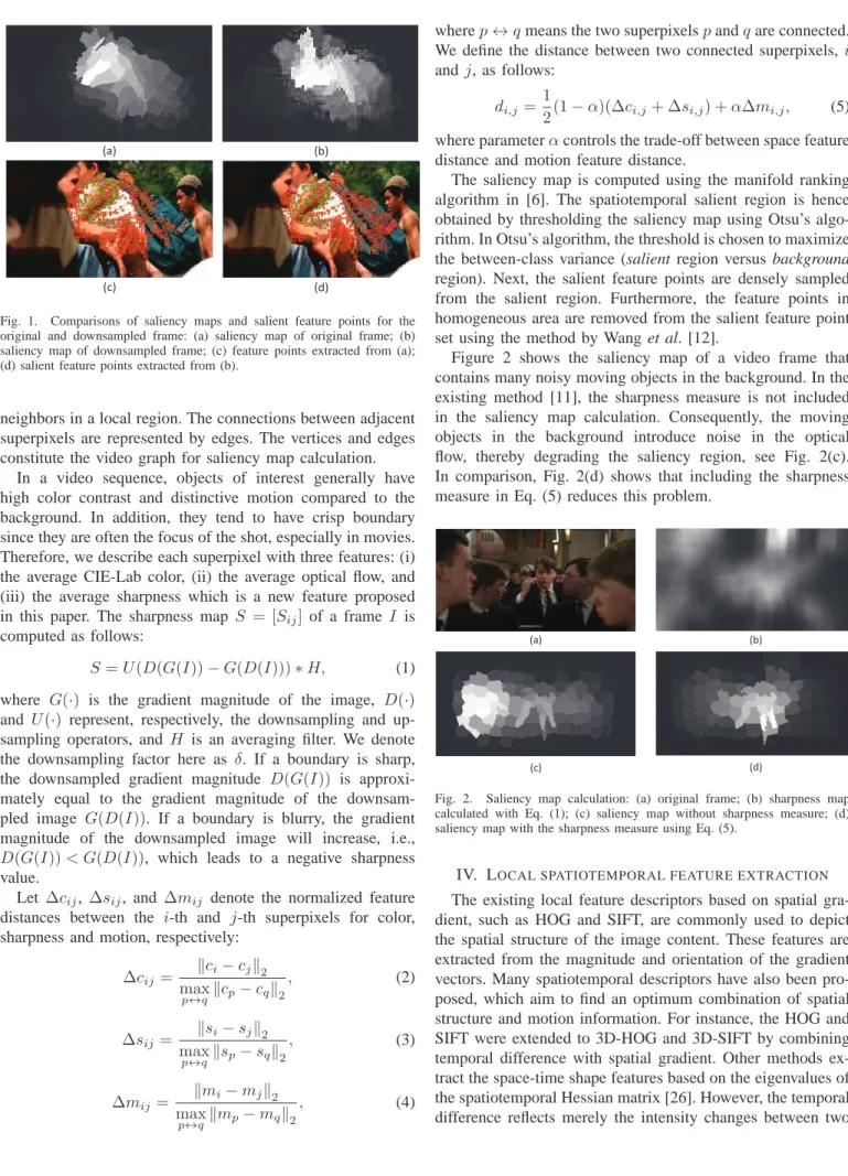
number of pixels. We reduce the computational cost of this step by downsampling the input frames. With this strategy, the segmentation of the original frame is the rescaled segmentation result of the downsampled frame. Superpixels generated with this method have rough boundary which, however, is not a significant problem for salient feature point detection. Figure 1 shows the saliency map and salient feature points for the original frame and downsampled frame. It can be seen that superpixels in the salient region have high values in both frames and the salient feature points have similar distribution.
If the original frame is downsampled by a factorδ= 1/W in
both dimensions, the computation cost is significantly reduced
by a factor1/W2.
B. Graph construction
In the graph-based manifold ranking method, superpixels are treated as vertices, and each vertex is connected to its
(a) (b)
(c) (d)
Fig. 1. Comparisons of saliency maps and salient feature points for the original and downsampled frame: (a) saliency map of original frame; (b) saliency map of downsampled frame; (c) feature points extracted from (a); (d) salient feature points extracted from (b).
neighbors in a local region. The connections between adjacent superpixels are represented by edges. The vertices and edges constitute the video graph for saliency map calculation.
In a video sequence, objects of interest generally have high color contrast and distinctive motion compared to the background. In addition, they tend to have crisp boundary since they are often the focus of the shot, especially in movies. Therefore, we describe each superpixel with three features: (i) the average CIE-Lab color, (ii) the average optical flow, and (iii) the average sharpness which is a new feature proposed
in this paper. The sharpness map S = [Sij] of a frame I is
computed as follows:
S=U(D(G(I))−G(D(I)))∗H, (1)
where G(·) is the gradient magnitude of the image, D(·)
and U(·) represent, respectively, the downsampling and
up-sampling operators, and H is an averaging filter. We denote
the downsampling factor here as δ. If a boundary is sharp,
the downsampled gradient magnitude D(G(I)) is
approxi-mately equal to the gradient magnitude of the
downsam-pled image G(D(I)). If a boundary is blurry, the gradient
magnitude of the downsampled image will increase, i.e., D(G(I))< G(D(I)), which leads to a negative sharpness value.
Let ∆cij, ∆sij, and∆mij denote the normalized feature
distances between the i-th and j-th superpixels for color,
sharpness and motion, respectively:
∆cij = kci−cjk2 max p↔q kcp−cqk2 , (2) ∆sij = ksi−sjk2 max p↔q ksp−sqk2 , (3) ∆mij = kmi−mjk2 max p↔qkmp−mqk2 , (4)
wherep↔qmeans the two superpixelspandqare connected.
We define the distance between two connected superpixels, i
andj, as follows:
di,j= 1
2(1−α)(∆ci,j+ ∆si,j) +α∆mi,j, (5)
where parameterαcontrols the trade-off between space feature
distance and motion feature distance.
The saliency map is computed using the manifold ranking algorithm in [6]. The spatiotemporal salient region is hence obtained by thresholding the saliency map using Otsu’s algo-rithm. In Otsu’s algorithm, the threshold is chosen to maximize the between-class variance (salient region versus background region). Next, the salient feature points are densely sampled from the salient region. Furthermore, the feature points in homogeneous area are removed from the salient feature point set using the method by Wang et al. [12].
Figure 2 shows the saliency map of a video frame that contains many noisy moving objects in the background. In the existing method [11], the sharpness measure is not included in the saliency map calculation. Consequently, the moving objects in the background introduce noise in the optical flow, thereby degrading the saliency region, see Fig. 2(c). In comparison, Fig. 2(d) shows that including the sharpness measure in Eq. (5) reduces this problem.
(a) (b)
(c) (d)
Fig. 2. Saliency map calculation: (a) original frame; (b) sharpness map calculated with Eq. (1); (c) saliency map without sharpness measure; (d) saliency map with the sharpness measure using Eq. (5).
IV. LOCAL SPATIOTEMPORAL FEATURE EXTRACTION
The existing local feature descriptors based on spatial gra-dient, such as HOG and SIFT, are commonly used to depict the spatial structure of the image content. These features are extracted from the magnitude and orientation of the gradient vectors. Many spatiotemporal descriptors have also been pro-posed, which aim to find an optimum combination of spatial structure and motion information. For instance, the HOG and SIFT were extended to 3D-HOG and 3D-SIFT by combining temporal difference with spatial gradient. Other methods ex-tract the space-time shape features based on the eigenvalues of the spatiotemporal Hessian matrix [26]. However, the temporal difference reflects merely the intensity changes between two
consecutive frames, which is not discriminative enough for motion description and is sensitive to the illumination changes. To address this problem, we propose to extract features from the motion surface, which is the combination of optical flow and spatial gradient.
On the motion surface, each pixel is represented with two vectors, the normal vector of the edge and the motion direction, which are related to the principal curvatures of surface at the pixel, see Fig. 3(a). The two vectors form a
hemispherical space, see Fig. 3(b), where the longitudeθis the
orientation of the optical flow and latitudeφis the orientation
of the gradient. The gradient orientation is in the range[0, π]
since the opposite direction of the gradient orientation refers to the same edge direction. Note that the orientation space model is different from the 3-D gradient model, c.f. Fig. 3(b)
and (c). In the 3-D gradient model, the longitudeθ andφare
separately calculated based on the gradient with two formulas θ= arctan(gt/gx)andφ= arctan(gy/
p gx2+g2
t), which are
not the measure of the motion direction. In contrast with the 3-D gradient model, features based on the orientation model will be more perceivable and more robust to the illumination changes. L N N n n n å Gradient Optical flow Gradient Orientation
Optical Flow Orientation
(a) Moving surface (b) Orientation space of the curvature (c) 3-D gradient model
q
j
x g y g t g å q jq
j
j
j
j
j
g y g t gq
j
Fig. 3. Motion surface curvature.
Let G(i, j, t) and V(i, j, t)be the gradient and optic flow
vector at position (i, j, t), respectively. The norm of the
curvature vector at this position is defined as
MC(i, j, t) =kG(i, j, t)k2 kV(i, j, t)k2. (6)
It can be observed that MC(i, j, t)has a large value only if
the point (i, j, t)is located on the edge (or at a corner) and
has distinct movement.
The orientations of the gradient and optical flow vectors
are separately quantized into Ng bins and No bins. For the
optical flow vector, a zero bin is added for pixels with small movement. As each point is described by two orientations, the local histogram around a feature point is a matrix of
size Ng×(No+ 1). We extract the histogram features of
the spatiotemporal orientation from each video cuboid with two new feature descriptors: STOH (spatiotemporal orientation histogram) and RISTOH (rotation invariant spatiotemporal orientation histogram), which are the extension of HOG and SIFT descriptors, respectively. The central axis of the video cuboid is the track of the salient feature point produced by Farneback’s optical flow algorithm. To extract STOH and
RISTOH features, we divide each cuboid into nσ×nσ×nτ
sub-blocks. The feature vectors of both STOH and RISTOH
for each sub-block are of length Ng×(No+ 1). Therefore,
the feature vectors of both STOH and RISTOH consist of
Ng ×(No + 1)×nσ ×nσ ×nτ elements. The dominant
orientation of RISTOH is the same as that of SIFT. Fig. 4 illustrates the method to extract STOH and RISTOH features from each video cuboid.
L N N ns ns nt t å STOH RISTOH t å Rotate and weight q j
Fig. 4. Illustration of the STOH and RISTOH feature descriptors.
V. EXPERIMENTS ANDRESULTS
To investigate the salient feature point detection method and the local feature descriptors STOH and RISTOH, experiments are conducted on three video datasets: KTH, YouTube, and Hollywood2. The three datasets are among the most widely used for video classification. In this section, we first give a brief description for these datasets, and introduce the experi-mental setup. We then compare the performance of different feature point detection methods and different local features.
A. Video datasets
The KTH dataset [27] contains six distinct actions: walking, jogging, running, boxing, waving and clapping. Each action is performed several times by 25 subjects. Videos from 9 subjects (2, 3, 5, 6, 7, 8, 9, 10, and 22) are used for testing and the remaining videos are used for training. This dataset contains 599 video sequences, each separated into about 4 sub-sequences. Each sub-sequence is treated as a sample and the total number of samples is 2391. The dataset contains a homogeneous background and controlled variations: outdoors with scale variation, outdoors with different clothes, and indoors.
The YouTube dataset [28] contains 11 action categories: basketball shooting, biking/cycling, diving, golf swinging, horse back riding, soccer juggling, swinging, tennis swinging, trampoline jumping, volleyball spiking, and walking with a dog. The dataset contains a total of 1,168 sequences, which are divided into 25 groups. The experiment on this dataset calculates the average classification rate by using Leave-One-Out Cross-Validation approach. This dataset is challenging due to large variations in camera motion, object appearance and pose, object scale, viewpoint, cluttered background and illumination conditions.
The Hollywood2 dataset [29] contains 12 action categories: answering the phone, driving car, eating, fighting, getting out of car, hand shaking, hugging, kissing, running, sitting down,
sitting up, and standing up. The dataset is collected from 69 different Hollywood movies. In total, there are 1,707 video sequences divided into a training set (823 sequences) and a test set (884 sequences). This video dataset is very challeng-ing since it has natural background, shot cuts, illumination changes, and co-occurrence of different actions.
B. Experimental method
In the process of saliency map calculation, the
down-sampling factorδis set to1/5. Letγbe a predefined threshold
which is set to1%of the maximum of image height and width.
Parameterαis set to 0.6 if the maximum magnitude of optical
flows is larger thanγ. Otherwise,αis set to 0.4 to make the
measurement robust to the optical flow noise. To calculate the
sharpness map, the downsampling factor δis set to 1/2, and
H is defined as a Gaussian filter (withσ= 4) of size20×20.
The size of the video cuboid isN×N×L, see Fig. 4.Lis
the length of the salient trajectory andN is the neighbor size.
The parameters for the experiments are: N = 32, Ng = 4,
No = 8, nσ = 2, nτ = 3, and L = 15. Besides STOH
and RISTOH, other features including salient trajectory (ST), HOG, HOF, MBH, SIFT are also extracted in our experiments.
The HOG and SIFT have Ng orientation bins. Both MBHx
and MBHy have No orientation bins, whilst HOF has an
additional zero bin besides the No orientation bins. For the
SIFT descriptor, the cuboid is divided into4×4×τsubblocks.
To represent the video sequence, we generate a visual vocabulary for each local feature with the k-means algorithm. The histogram vector for each feature descriptor is a channel of the video. As there are different features, each video is represented by multi-channels. The dissimilarity between two
videos i and j on channel c is measured by the chi-squared
(χ2)distance: D(Hic, H c j) = 1 2 V X n=1 (hc i,n−h c j,n)2 hi,n+hj,n (7) where Hc i = [h c
i,n] is the histogram vector of channel c for
thei-th video,V is the vocabulary size, andnis the index of
a vocabulary word. For classification, we use non-linear SVM with multi-Gaussian kernel:
K(Hi, Hj) = exp − X c∈C 1 Ac Dc(Hc i, H c j) ! . (8)
where Ac is the average distance of the channelc.
C. Classification results
Three sets of experiment were conducted to investigate the performances of different feature detection methods and different local feature descriptors. In the first set of experi-ment, we assess the performance of feature point detection methods in terms of the number of salient points detected and classification accuracy. Table I lists two performance measures for three feature point detection methods: dense sampling (DS) [12], motion boundary of dense sampling (DS-MB) [14], and salient sampling (SS) method. The number of feature points
per frame indicates the density of features sampled from the video sequence. The classification rate (CR) is obtained by using the same feature combination (HOG, HOF, and MBH) on a vocabulary size of 4000. The experiment results of dense sampling method and motion boundary of dense sampling method are produced by us repeating the experiments of [12] and [14]; the results may differ slightly from the original references, but the difference is not significant for our analysis. The proposed SS has a higher CR than DS on the KTH dataset (95.1% vs 94.2%) and and the YouTube dataset (85.1% vs 84.3%). SS also uses only half the number of feature points compared to DS. Note that DS produces many noisy features in the background region. This result indicates that noisy background features degrade the classification accuracy, and hence should be removed. The DS-MB uses the smaller number of feature points per frame, but it also has the lowest classification rate on both datasets.
TABLE I
PERFORMANCE MEASURES OF DIFFERENT FEATURE POINT DETECTION METHODS ON THEKTHANDYOUTUBE DATASETS.
Datasets Methods Feature points/frame CR (%)
KTH DS 256.6 94.2 DS-MB 144 93.8 SS 157.5 95.1 YouTube DS 1066.2 84.3 DS-MB 302.4 83.4 SS 559.6 85.1
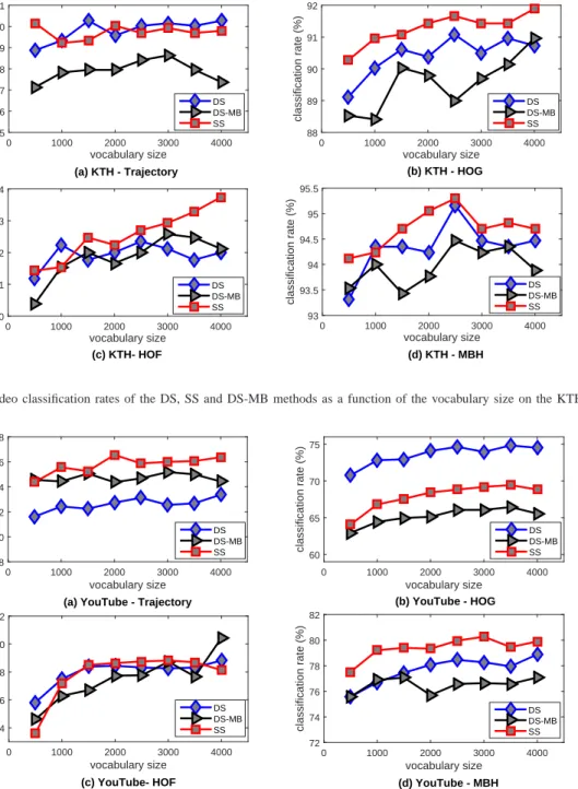
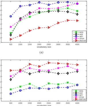
Figures 5 and 6 show the classification rates of DS, DS-MB, and SS on the KTH and YouTube datasets, across different vocabulary sizes (500 to 4000) and feature descriptors (HOG, HOF, MBH, and point trajectory). The DS-BM method has lower classification rates than the DS and SS methods. This applies to all feature descriptors, except for the trajectory descriptor on the YouTube dataset. Note that DS-MB retains only the feature points near the moving boundary, and removes feature points which may contain distinct properties of the background and objects. The proposed method (SS) has higher classification rates than the DS and DS-BM methods on both datasets, except for the HOG descriptor on the YouTube dataset. Compared with DS-MB, the SS method keeps more feature points located in the salient region. Since the saliency map is calculated by comparing the color distance, optical flow distance, and sharpness distance, objects of interest are kept in the salient region even though their motions are not dominant. In the second set of experiment, we evaluate the classifi-cation performance of the proposed descriptors (STOH and RISTOH) and compare them with the existing descriptors (HOG, HOF, and SIFT). The descriptors are extracted from the salient feature points and the vocabulary size is varied from 500 to 4000. The results on the YouTube and Hollywood2 dataset are shown in Fig. 7. It can be seen that STOH yields higher CRs than HOG and HOF on both Hollywood2 and YouTube datasets, at almost all vocabulary sizes. This indicates that the features extracted from the curvature are more dis-criminative than those extracted from spatial gradient. Among
vocabulary size 0 1000 2000 3000 4000 classification rate (%) 85 86 87 88 89 90 91 (a) KTH - Trajectory DS DS-MB SS vocabulary size 0 1000 2000 3000 4000 classification rate (%) 88 89 90 91 92 (b) KTH - HOG DS DS-MB SS vocabulary size 0 1000 2000 3000 4000 classification rate (%) 90 91 92 93 94 (c) KTH- HOF DS DS-MB SS vocabulary size 0 1000 2000 3000 4000 classification rate (%) 93 93.5 94 94.5 95 95.5 (d) KTH - MBH DS DS-MB SS
Fig. 5. The video classification rates of the DS, SS and DS-MB methods as a function of the vocabulary size on the KTH dataset.
vocabulary size 0 1000 2000 3000 4000 classification rate (%) 58 60 62 64 66 68
(a) YouTube - Trajectory DS DS-MB SS vocabulary size 0 1000 2000 3000 4000 classification rate (%) 60 65 70 75 (b) YouTube - HOG DS DS-MB SS vocabulary size 0 1000 2000 3000 4000 classification rate (%)64 66 68 70 72 (c) YouTube- HOF DS DS-MB SS vocabulary size 0 1000 2000 3000 4000 classification rate (%) 72 74 76 78 80 82 (d) YouTube - MBH DS DS-MB SS
Fig. 6. The video classification rates of the DS, SS and DS-MB methods as a function of the vocabulary size on the YouTube dataset.
the evaluated descriptors, the SIFT descriptor performs the best in the YouTube dataset and the worst in the Hollywood2 dataset. The RISTOH descriptor performs the worst in the YouTube dataset and the best in the Hollywood2 dataset. These results indicate that the discriminative power of rotation-invariant features is not stable and depends significantly on the properties of the dataset. It can be observed that in the YouTube dataset, the sport categories are highly correlated to the scene background. In Hollywood2 dataset, the action categories mainly depend the human motions. This could explain that the SIFT descriptor has a higher CR in the
YouTube dataset and the RISTOH descriptor has a higher CR in the Hollywood2 dataset.
In the third set of experiment, we evaluate different combinations of features to classify the videos in all three datasets and compare with some recent state-of-the-art meth-ods in action recognition. The classification rates from the best combinations are shown in Table II, together with results from other methods. We found that the best combination of features depends on the dataset. For example, STOH plus MBH gives the highest CR on the KTH dataset, whereas RISTOH in combination with HOF, MBH, and ST yields
vocabulary size 500 1000 1500 2000 2500 3000 3500 4000 classification rate (%) 62 63 64 65 66 67 68 69 70 71 HOG HOF SIFT STOH RISTOH (a) vocabulary size 500 1000 1500 2000 2500 3000 3500 4000 classification rate (%) 38 40 42 44 46 48 50 52 HOG HOF SIFT STOH RISTOH (b)
Fig. 7. Video classification rates as a function of the vocabulary size for different feature descriptors on two datasets: (a) YouTube, and (b) Hollywood2.
the highest CR on the Hollywood2 dataset. It is notable that the classification rate on the KTH dataset decreases when more features are combined. The background in KTH is homogeneous so the discriminative information is easily depicted by each local feature descriptor. The combination of multiple features introduces more noise to the feature set while not increasing significantly the discriminative features. As a consequence, it leads to a lower classification rate than the combination of fewer features.
TABLE II
THE CLASSIFICATION RATE(%)OF DIFFERENT METHODS ON THREE VIDEO DATASETS.
Method KTH YouTube Hollywood2
ISA [15] 93.9 75.8 53.3 DT + HOG + HOF + MBH [12] 95.0 84.1 58.2 Harris3D + HOG/HOF [30] 91.8 - 45.2 STOH + MBH 95.1 83.2 57.5 ST + SIFT + HOF + MBH 94.3 85.6 58.4 ST + RISTOH + HOF + MBH 93.8 84.5 58.7 VI. CONCLUSION
In this paper, we propose a method to detect feature points from the salient region to remove the noisy background points from the densely sampled feature point set. An extension of graph-based manifold ranking method is developed to detect the salient feature points in a video sequence more efficiently. The experimental results show that the salient trajectory leads to a more compact and more discriminative feature set. Two
new features, named as STOH and RISTOH, are proposed based on the spatiotemporal orientation model of the motion surface, which is a combination of spatial gradient and optical flow. The proposed feature descriptor, STOH performs better in terms of classification rate than HOG and HOF, which indi-cates that features extracted from the spatiotemporal structure of the video content are more discriminative than the features extracted from the spatial structure. The other proposed feature descriptor RISTOH has better performance than SIFT in the KTH and Hollywood2 datasets whilst degrades in the YouTube dataset. The performance of SIFT and RISTOH suggests that the rotation invariant features are highly related to the dataset properties.
ACKNOWLEDGMENT
Xiaolin Tang is supported by a PhD scholarship from the Chinese Scholarship Council (NO. 201306370047). This research is supported by a grant from the Australian Research Council.
REFERENCES
[1] C.-R. Huang, Y.-J. Chang, Z.-X. Yang, and Y.-Y. Lin, “Video saliency map detection by dominant camera motion removal,” IEEE Transactions
on Circuits and Systems for Video Technology, vol. 24, no. 8, pp. 1336–
1349, 2014.
[2] J. Harel, C. Koch, and P. Perona, “Graph-based visual saliency,” in Proc.
Advances in Neural Information Processing Systems, 2006, pp. 545–552.
[3] T. Liu, Z. Yuan, J. Sun, J. Wang, N. Zheng, X. Tang, and H. Y. Shum, “Learning to detect a salient object,” IEEE Transactions on Pattern
Analysis and Machine Intelligence, vol. 33, no. 2, pp. 353–367, 2011.
[4] M.-M. Cheng, G.-X. Zhang, N. J. Mitra, X. Huang, and S.-M. Hu, “Global contrast based salient region detection,” in Proc. IEEE
Confer-ence on Computer Vision and Pattern Recognition, 2011, pp. 409–416.
[5] F. Perazzi, P. Krahenbuhl, Y. Pritch, and A. Hornung, “Saliency filters: Contrast based filtering for salient region detection,” in Proc. IEEE
Conference on Computer Vision and Pattern Recognition, 2012, pp. 733–
740.
[6] C. Yang, L. Zhang, H. Lu, X. Ruan, and M.-H. Yang, “Saliency detection via graph-based manifold ranking,” in Proc. IEEE Conference
on Computer Vision and Pattern Recognition, 2013, pp. 3166–3173.
[7] S. Goferman, L. Zelnik-Manor, and A. Tal, “Context-aware saliency detection,” IEEE Transactions on Pattern Analysis and Machine
Intelli-gence, vol. 34, no. 10, pp. 1915–1926, 2012.
[8] G. Zhi, C. Loong-Fah, and W. Yu-Xiang, “Block-sparse RPCA for salient motion detection,” IEEE Transactions on Pattern Analysis and
Machine Intelligence, vol. 36, no. 10, pp. 1975–1987, 2014.
[9] V. Mahadevan and N. Vasconcelos, “Spatiotemporal saliency in dynamic scenes,” IEEE Transactions on Pattern Analysis and Machine
Intelli-gence, vol. 32, no. 1, pp. 171–177, 2010.
[10] H. Kim, Y. Kim, J. Sim, and C. Kim, “Spatiotemporal saliency detection for video sequences based on random walk with restart,” IEEE
Trans-actions on Image Processing, vol. 24, no. 8, pp. 2552–2564, 2015.
[11] K. Fu, I. Y. H. Gu, Y. Yixiao, G. Chen, and Y. Jie, “Graph construction for salient object detection in videos,” in Proc. IEEE International
Conference on Pattern Recognition, 2014, pp. 2371–2376.
[12] H. Wang, A. Klser, C. Schmid, and C.-L. Liu, “Dense trajectories and motion boundary descriptors for action recognition,” International
Journal of Computer Vision, vol. 103, no. 1, pp. 60–79, 2013.
[13] J. Sun, X. Wu, S. Yan, L.-F. Cheong, T.-S. Chua, and J. Li, “Hierarchical spatio-temporal context modeling for action recognition,” in Proc. IEEE
Conference on Computer Vision and Pattern Recognition., 2009, pp.
2004–2011.
[14] X. Peng, Y. Qiao, Q. Peng, and X. Qi, “Exploring motion boundary based sampling and spatial-temporal context descriptors for action recognition,” in Proc. British Machine Vision Conference, 2013, pp. 1– 11.
[15] Q. Le, W. Zou, S. Yeung, and A. Ng, “Learning hierarchical invariant spatio-temporal features for action recognition with independent sub-space analysis,” in Proc. IEEE Conference on Computer Vision and
Pattern Recognition, 2011, pp. 3361–3368.
[16] M. Oquab, L. Bottou, I. Laptev, and J. Sivic, “Learning and transferring mid-level image representations using convolutional neural networks,” in Proc. IEEE Conference on Computer Vision and Pattern Recognition, 2011, pp. 1717–1724.
[17] S. Chatzis, “A nonparametric Bayesian approach toward stacked convolutional independent component analysis,” CoRR, vol. abs/1411.4423, 2014. [Online]. Available: http://arxiv.org/abs/1411.4423 [18] P. Matikainen, M. Hebert, and R. Sukthankar, “Trajectons: Action recognition through the motion analysis of tracked features,” in Proc.
IEEE International Conference on Computer Vision Workshops, 2009,
pp. 514–521.
[19] J. Donahue, L. A. Hendricks, S. Guadarrama, M. Rohrbach, S. Venugopalan, K. Saenko, and T. Darrell, “Long-term recurrent convolutional networks for visual recognition and description,” CoRR, vol. abs/1411.4389, 2014. [Online]. Available: http://arxiv.org/abs/1411.4389
[20] Z. Wu, X. Wang, Y. Jiang, H. Ye, and X. Xue, “Modeling spatial-temporal clues in a hybrid deep learning framework for video classification,” CoRR, vol. abs/1504.01561, 2015. [Online]. Available: http://arxiv.org/abs/1504.01561
[21] R. Messing, C. Pal, and H. Kautz, “Activity recognition using the velocity histories of tracked keypoints,” in Proc. IEEE International
Conference on Computer Vision, 2009, pp. 104–111.
[22] N. Dalal, B. Triggs, and C. Schmid, “Human detection using oriented
histograms of flow and appearance,” in Proc. European Conference on
Computer Vision, 2006, pp. 428–441.
[23] N. Buch, J. Orwell, and S. A. Velastin, “3D extended histogram of oriented gradients (3DHOG) for classification of road users in urban scenes,” in Proc. ITS World Conference, 2009, pp. 1–8.
[24] P. Scovanner, S. Ali, and M. Shah, “A 3-dimensional sift descriptor and its application to action recognition,” in Proc. ACM International
Conference on Multimedia, 2007, pp. 357–360.
[25] R. Achanta, A. Shaji, K. Smith, A. Lucchi, P. Fua, and S. Susstrunk, “Slic superpixels compared to state-of-the-art superpixel methods,” IEEE
Transactions on Pattern Analysis and Machine Intelligence, vol. 34,
no. 11, pp. 2274–2282, 2012.
[26] M. Blank, L. Gorelick, E. Shechtman, M. Irani, and R. Basri, “Actions as space-time shapes,” in Proc. IEEE International Conference on
Computer Vision, vol. 2, 2005, pp. 1395–1402.
[27] C. Sch¨uldt, I. Laptev, and B. Caputo, “Recognizing human actions: a local SVM approach,” in Proc. IEEE International Conference on
Pattern Recognition, vol. 3, 2004, pp. 32–36.
[28] J. Liu, J. Luo, and M. Shah, “Recognizing realistic actions from videos in the wild,” in Proc. IEEE Conference on Computer Vision and Pattern
Recognition, 2009, pp. 1996–2003.
[29] M. Marszałek, I. Laptev, and C. Schmid, “Actions in context,” in Proc.
IEEE Conference on Computer Vision and Pattern Recognition, 2009,
pp. 2929–2936.
[30] H. Wang, M. M. Ullah, A. Klaser, I. Laptev, and C. Schmid, “Evaluation of local spatio-temporal features for action recognition,” in Proc. British