PyMC: Bayesian Stochastic Modelling in Python

July 2010, Volume 35, Issue 4. http://www.jstatsoft.org/

PyMC

: Bayesian Stochastic Modelling in

Python

This user guide describes a Python package, PyMC, that allows users to efficiently code a probabilistic model and draw samples from its posterior distribution using Markov chain Monte Carlo techniques.

Keywords: Bayesian modeling, Markov chain Monte Carlo, simulation,Python.

1. Introduction

1.1. Purpose

PyMCis a python module that implements Bayesian statistical models and fitting algorithms, including Markov chain Monte Carlo. Its flexibility and extensibility make it applicable to a large suite of problems. Along with core sampling functionality,PyMC includes methods for summarizing output, plotting, goodness-of-fit and convergence diagnostics.

1.2. Features

PyMC provides functionalities to make Bayesian analysis as painless as possible. It fits Bayesian statistical models with Markov chain Monte Carlo and other algorithms. Traces can be saved to the disk as plain text, Python pickles, SQLite (The SQLite Development Team 2010) or MySQL (Oracle Corporation 2010) database, or HDF5 (The HDF Group 2010) archives. Summaries including tables and plots can be created from these, and several convergence diagnostics are available. Sampling loops can be paused and tuned manually, or saved and restarted later. MCMC loops can be embedded in larger programs, and results can be analyzed with the full power of Python.

PyMC includes a large suite of well-documented statistical distributions which use NumPy (Oliphant 2006) and hand-optimized Fortran routines wherever possible for performance. It

also includes a module for modeling Gaussian processes. Equally importantly, PyMC can easily be extended with custom step methods and unusual probability distributions.

1.3. Usage

First, define your model in a file, say mymodel.py:

import pymc

import numpy as np

n = 5*np.ones(4,dtype=int)

x = np.array([-.86,-.3,-.05,.73])

alpha = pymc.Normal('alpha',mu=0,tau=.01) beta = pymc.Normal('beta',mu=0,tau=.01) @pymc.deterministic

def theta(a=alpha, b=beta):

"""theta = logit^{-1}(a+b)""" return pymc.invlogit(a+b*x)

d = pymc.Binomial('d', n=n, p=theta, value=np.array([0.,1.,3.,5.]),\ observed=True)

Save this file, then from aPython shell (or another file in the same directory), call:

import pymc import mymodel

S = pymc.MCMC(mymodel, db = 'pickle')

S.sample(iter = 10000, burn = 5000, thin = 2) pymc.Matplot.plot(S)

This example will generate 10000 posterior samples, thinned by a factor of 2, with the first half discarded as burn-in. The sample is stored in aPythonserialization (pickle) database.

1.4. History

PyMCbegan development in 2003, as an effort to generalize the process of building Metropolis-Hastings samplers, with an aim to making Markov chain Monte Carlo (MCMC) more acces-sible to non-statisticians (particularly ecologists). The choice to develop PyMC as aPython module, rather than a standalone application, allowed the use MCMC methods in a larger modeling framework. By 2005, PyMC was reliable enough for version 1.0 to be released to the public. A small group of regular users, most associated with the University of Georgia, provided much of the feedback necessary for the refinement ofPyMCto a usable state. In 2006, David Huard and Anand Patil joined Chris Fonnesbeck on the development team for PyMC2.0. This iteration of the software strives for more flexibility, better performance and a better end-user experience than any previous version ofPyMC.

PyMC2.1 has been released in early 2010. It contains numerous bugfixes and optimizations, as well as a few new features. This user guide is written for version 2.1.

1.5. Relationship to other packages

PyMCin one of many general-purpose MCMC packages. The most prominent among them is WinBUGS(Spiegelhalter, Thomas, Best, and Lunn 2003;Lunn, Thomas, Best, and Spiegel-halter 2000), which has made MCMC and with it Bayesian statistics accessible to a huge user community. UnlikePyMC,WinBUGSis a stand-alone, self-contained application. This can be an attractive feature for users without much programming experience, but others may find it constraining. A related package is JAGS (Plummer 2003), which provides a more Unix-like implementation of the BUGS language. Other packages includeHierarchical Bayes Compiler(Daum´e III 2007) and a number of R (RDevelopment Core Team 2010) packages, for example MCMCglmm(Hadfield 2010) andMCMCpack(Martin, Quinn, and Park 2009). It would be difficult to meaningfully benchmarkPyMC against these other packages because of the unlimited variety in Bayesian probability models and flavors of the MCMC algorithm. However, it is possible to anticipate how it will perform in broad terms.

PyMC’s number-crunching is done using a combination of industry-standard libraries (NumPy,

Oliphant 2006, and the linear algebra libraries on which it depends) and hand-optimized For-tranroutines. For models that are composed of variables valued as large arrays, PyMC will spend most of its time in these fast routines. In that case, it will be roughly as fast as pack-ages written entirely in C and faster than WinBUGS. For finer-grained models containing mostly scalar variables, it will spend most of its time in coordinating Python code. In that case, despite our best efforts at optimization,PyMCwill be significantly slower than packages written in Cand on par with or slower than WinBUGS. However, as fine-grained models are often small and simple, the total time required for sampling is often quite reasonable despite this poorer performance.

We have chosen to spend time developing PyMC rather than using an existing package pri-marily because it allows us to build and efficiently fit any model we like within a full-fledged Python environment. We have emphasized extensibility throughout PyMC’s design, so if it doesn’t meet your needs out of the box chances are you can make it do so with a relatively small amount of code. See the testimonials page (http://code.google.com/p/pymc/wiki/ Testimonials) for reasons why other users have chosen PyMC.

1.6. Getting started

This guide provides all the information needed to install PyMC, code a Bayesian statistical model, run the sampler, save and visualize the results. In addition, it contains a list of the statistical distributions currently available. More examples of usage as well as tutorials are available from the PyMCweb site athttp://code.google.com/p/pymc.

2. Installation

2.1. Dependencies

are currently only a few dependencies, and all are freely available online.

ˆ Python version 2.5 or 2.6.

ˆ NumPy (1.4 or newer): The fundamental scientific programming package, it provides a multidimensional array type and many useful functions for numerical analysis.

ˆ matplotlib (Hunter 2007), optional: 2D plotting library which produces publication quality figures in a variety of image formats and interactive environments

ˆ PyTables (Alted, Vilata, Prater, Mas, Hedley, Valentino, and Whitaker 2010), optional: Package for managing hierarchical datasets and designed to efficiently and easily cope with extremely large amounts of data. Requires theHDF5 library.

ˆ pydot (Carrera and Theune 2010), optional: Python interface to Graphviz (Gansner and North 1999), it allows PyMC to create both directed and non-directed graphical representations of models.

ˆ SciPy (Jones, Oliphant, and Peterson 2001), optional: Library of algorithms for math-ematics, science and engineering.

ˆ IPython(P´erez and Granger 2007) , optional: An enhanced interactivePythonshell and an architecture for interactive parallel computing.

ˆ nose (Pellerin 2010), optional: A test discovery-based unittest extension (required to run the test suite).

There are prebuilt distributions that include all required dependencies. For Mac OS X users, we recommend the MacPython (Python Software Foundation 2005) distribution or the En-thoughtPythondistribution (Enthought, Inc. 2010) on OS X 10.5 (Leopard) andPython2.6.1 that ships with OS X 10.6 (Snow Leopard). Windows users should download and install the EnthoughtPython Distribution. The EnthoughtPythondistribution comes bundled with these prerequisites. Note that depending on the currency of these distributions, some packages may need to be updated manually.

If instead of installing the prebuilt binaries you prefer (or have) to build PyMC yourself, make sure you have aFortranand aCcompiler. There are free compilers (gfortran,gcc,Free Software Foundation, Inc. 2010) available on all platforms. Other compilers have not been tested withPyMC but may work nonetheless.

2.2. Installation using EasyInstall

The easiest way to installPyMC is to type in a terminal:

easy_install pymc

Provided EasyInstall (part of the setuptools module, Eby 2010) is installed and in your path, this should fetch and install the package from the Python Package Index at http: //pypi.python.org/pypi. Make sure you have the appropriate administrative privileges to install software on your computer.

2.3. Installing from pre-built binaries

Pre-built binaries are available for Windows XP and Mac OS X. There are at least two ways to install these. First, you can download the installer for your platform from the Python Package Index. Alternatively, you can double-click the executable installation package, then follow the on-screen instructions.

For other platforms, you will need to build the package yourself from source. Fortunately, this should be relatively straightforward.

2.4. Compiling the source code

First, download the source code tarball from thePython Package Index and unpack it. Then move into the unpacked directory and follow the platform specific instructions.

Windows

One way to compile PyMC on Windows is to install MinGW (Peters 2010) and MSYS. MinGWis the GNU Compiler Collection (gcc) augmented with Windows specific headers and libraries. MSYS is a POSIX-like console (bash) with Unix command line tools. Download the Automated MinGW Installer from http://sourceforge.net/projects/mingw/files/ and double-click on it to launch the installation process. You will be asked to select which components are to be installed: make sure the g77 (Free Software Foundation, Inc. 2010) compiler is selected and proceed with the instructions. Then download and install http: //downloads.sourceforge.net/mingw/MSYS-1.0.11.exe, launch it and again follow the on-screen instructions.

Once this is done, launch the MSYS console, change into thePyMCdirectory and type:

python setup.py install

This will build theC andFortran extension and copy the libraries andPythonmodules in the C:/Python26/Lib/site-packages/pymcdirectory.

Mac OS X or Linux

In a terminal, type:

python setup.py config_fc --fcompiler=gnu95 build python setup.py install

The above syntax also assumes that you have gfortran installed and available. The sudo command may be required to install PyMC into the Python site-packages directory if it has restricted privileges.

2.5. Development version

You can clone out the bleeding edge version of the code from thegit(Torvalds 2010) repository:

2.6. Running the test suite

PyMCcomes with a set of tests that verify that the critical components of the code work as expected. To run these tests, users must havenose installed. The tests are launched from a Python shell:

import pymc pymc.test()

In case of failures, messages detailing the nature of these failures will appear.

2.7. Bugs and feature requests

Report problems with the installation, test failures, bugs in the code or feature request on the issue tracker at http://code.google.com/p/pymc/issues/list, specifying the version you are using and the environment. Comments and questions are welcome and should be addressed to PyMC’s mailing list at [email protected].

3. Tutorial

This tutorial will guide you through a typical PyMCapplication. Familiarity with Pythonis assumed, so if you are new toPython, books such asLutz(2007) orLangtangen(2009) are the place to start. Plenty of online documentation can also be found on thePythondocumentation page at http://www.python.org/doc/.

3.1. An example statistical model

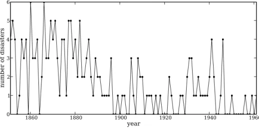
Consider a sample dataset consisting of a time series of recorded coal mining disasters in the UK from 1851 to 1962 (Figure 1, Jarrett 1979). Occurrences of disasters in the series is

1860 1880 1900 1920 1940 1960 year 0 1 2 3 4 5 6 number of disasters

thought to be derived from a Poisson process with a large rate parameter in the early part of the time series, and from one with a smaller rate in the later part. We are interested in locating the change point in the series, which perhaps is related to changes in mining safety regulations.

We represent our conceptual model formally as a statistical model:

(Dt|s, e, l)∼Poisson (rt), rt= e if t < s l if t≥s , t∈[tl, th] s∼Discrete Uniform(tl, th) e∼Exponential(re) l∼Exponential(rl) (1)

The symbols are defined as:

Dt: The number of disasters in year t.

rt: The rate parameter of the Poisson distribution of disasters in yeart.

s: The year in which the rate parameter changes (the switchpoint).

e: The rate parameter before the switchpoints.

l: The rate parameter after the switchpoints.

tl, th: The lower and upper boundaries of yeart.

re, rl: The rate parameters of the priors of the early and late rates, respectively.

Because we have definedDby its dependence ons,eand l, the latter three are known as the ‘parents’ ofD and Dis called their ‘child’. Similarly, the parents of sare tl and th, andsis

the child of tl and th.

3.2. Two types of variables

At the model-specification stage (before the data are observed),D,s,e,randlare all random variables. Bayesian ‘random’ variables have not necessarily arisen from a physical random process. The Bayesian interpretation of probability is epistemic, meaning random variable

x’s probability distribution p(x) represents our knowledge and uncertainty about x’s value (Jaynes 2003). Candidate values of x for which p(x) is high are relatively more probable, given what we know. Random variables are represented inPyMCby the classesStochastic andDeterministic.

The onlyDeterministicin the model isr. If we knew the values ofr’s parents (s,lande), we could compute the value of r exactly. A Deterministic liker is defined by a mathematical function that returns its value given values for its parents. Deterministic variables are sometimes called thesystemicpart of the model. The nomenclature is a bit confusing, because these objects usually represent random variables; since the parents of r are random, r is random also. A more descriptive (though more awkward) name for this class would be DeterminedByValuesOfParents.

On the other hand, even if the values of the parents of variabless, D (before observing the data), e or l were known, we would still be uncertain of their values. These variables are

characterized by probability distributions that express how plausible their candidate values are, given values for their parents. TheStochasticclass represents these variables. A more descriptive name for these objects might beRandomEvenGivenValuesOfParents.

We can represent model1 in a file calledDisasterModel.py (the actual file can be found in pymc/examples/) as follows. First, we import thePyMC and NumPynamespaces:

from pymc import DiscreteUniform, Exponential, deterministic, Poisson, Uniform import numpy

Notice that from pymc we have only imported a select few objects that are needed for this particular model, whereas the entirenumpynamespace has been imported.

Next, we enter the actual data values into an array:

disasters_array = \ numpy.array([ 4, 5, 4, 0, 1, 4, 3, 4, 0, 6, 3, 3, 4, 0, 2, 6, 3, 3, 5, 4, 5, 3, 1, 4, 4, 1, 5, 5, 3, 4, 2, 5, 2, 2, 3, 4, 2, 1, 3, 2, 2, 1, 1, 1, 1, 3, 0, 0, 1, 0, 1, 1, 0, 0, 3, 1, 0, 3, 2, 2, 0, 1, 1, 1, 0, 1, 0, 1, 0, 0, 0, 2, 1, 0, 0, 0, 1, 1, 0, 2, 3, 3, 1, 1, 2, 1, 1, 1, 1, 2, 4, 2, 0, 0, 1, 4, 0, 0, 0, 1, 0, 0, 0, 0, 0, 1, 0, 0, 1, 0, 1])

Note that you don’t have to type in this entire array to follow along; the code is available in the source tree, in pymc/examples/DisasterModel.py. Next, we create the switchpoint variables:

s = DiscreteUniform('s', lower=0, upper=110, doc='Switchpoint[year]')

DiscreteUniformis a subclass of Stochasticthat represents uniformly-distributed discrete variables. Use of this distribution suggests that we have no preferencea priori regarding the location of the switchpoint; all values are equally likely. Now we create the exponentially-distributed variableseand lfor the early and late Poisson rates, respectively:

e = Exponential('e', beta=1) l = Exponential('l', beta=1)

Next, we define the variabler, which selects the early rate efor times before s and the late ratel for times after s. We create r using the deterministic decorator, which converts the ordinary Pythonfunctionr into a Deterministic object.

@deterministic(plot=False) def r(s=s, e=e, l=l):

""" Concatenate Poisson means """

out = numpy.empty(len(disasters_array)) out[:s] = e

out[s:] = l return out

The last step is to define the number of disastersD. This is a stochastic variable, but unlike

s, e and l we have observed its value. To express this, we set the argument observed to True (it is set to Falseby default). This tells PyMC that this object’s value should not be changed:

D = Poisson('D', mu=r, value=disasters_array, observed=True)

3.3. Why are data and unknown variables represented by the same object? Since it is represented by aStochasticobject,Dis defined by its dependence on its parentr

even though its value is fixed. This isn’t just a quirk ofPyMC’s syntax; Bayesian hierarchical notation itself makes no distinction between random variables and data. The reason is simple: to use Bayes’ theorem to compute the posterior p(e, s, l|D) of model (1), we require the likelihoodp(D|e, s, l). Even thoughD’s value is known and fixed, we need to formally assign it a probability distribution as if it were a random variable. Remember, the likelihood and the probability function are essentially the same, except that the former is regarded as a function of the parameters and the latter as a function of the data.

This point can be counterintuitive at first, as many peoples’ instinct is to regard data as fixed a priori and unknown variables as dependent on the data. One way to understand this is to think of statistical models like (1) as predictive models for data, or as models of the processes that gave rise to data. Before observing the value ofD, we could have sampled from its prior predictive distribution p(D) (i.e., the marginal distribution of the data) as follows:

1. Samplee,sand l from their priors. 2. SampleDconditional on these values.

Even after we observe the value of D, we need to use this process model to make inferences aboute,sandlbecause its the only information we have about how the variables are related. 3.4. Parents and children

We have above created a PyMC probability model, which is simply a linked collection of variables. To see the nature of the links, import or run DisasterModel.py and examines’s parents attribute from the Pythonprompt:

>>> from pymc.examples import DisasterModel >>> DisasterModel.s.parents

{`lower': 0, 'upper': 110}

The parents dictionary shows us the distributional parameters of s, which are constants. Now let’s examinine D’s parents:

>>> DisasterModel.D.parents

{`mu': <pymc.PyMCObjects.Deterministic 'r' at 0x3e51a70>}

We are using r as a distributional parameter ofD (i.e.,r is D’s parent). D internally labels

r as mu, meaning r plays the role of the rate parameter in D’s Poisson distribution. Now examine r’s childrenattribute:

r D mu e e l l s s

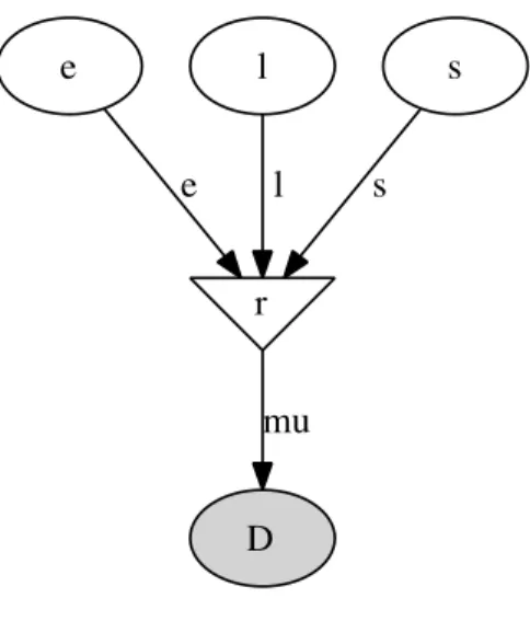
Figure 2: Directed acyclic graph of the relationships in the coal mining disaster model exam-ple.

>>> DisasterModel.r.children

set([<pymc.distributions.Poisson 'D' at 0x3e51290>])

Because D considers r its parent, r considers D its child. Unlike parents, children is a set (an unordered collection of objects); variables do not associate their children with any particular distributional role. Try examining the parents and children attributes of the other parameters in the model.

A ‘directed acyclic graph’ is a visualization of the parent-child relationships in the model. For example, in Figure 2 unobserved stochastic variables s,e and l are represented by open ellipses, observed stochastic variable D is a filled ellipse and deterministic variable r is a triangle. Arrows point from parent to child and display the label that the child assigns to the parent. See Section4.12 for more details.

As the examples above have shown, PyMC objects need to have a name assigned, such as lower,upper ore. These names are used for storage and post-processing:

ˆ as keys in on-disk databases,

ˆ as node labels in model graphs,

ˆ as axis labels in plots of traces,

ˆ as table labels in summary statistics.

A model instantiated with variables having identical names raises an error to avoid name conflicts in the database storing the traces. In general however,PyMCuses references to the objects themselves, not their names, to identify variables.

3.5. Variables’ values and log-probabilities

All PyMC variables have an attribute called value that stores the current value of that variable. Try examiningD’s value, and you’ll see the initial value we provided for it:

>>> DisasterModel.D.value array([4, 5, 4, 0, 1, 4, 3, 4, 0, 6, 3, 3, 4, 0, 2, 6, 3, 3, 5, 4, 5, 3, 1, 4, 4, 1, 5, 5, 3, 4, 2, 5, 2, 2, 3, 4, 2, 1, 3, 2, 2, 1, 1, 1, 1, 3, 0, 0, 1, 0, 1, 1, 0, 0, 3, 1, 0, 3, 2, 2, 0, 1, 1, 1, 0, 1, 0, 1, 0, 0, 0, 2, 1, 0, 0, 0, 1, 1, 0, 2, 3, 3, 1, 1, 2, 1, 1, 1, 1, 2, 4, 2, 0, 0, 1, 4, 0, 0, 0, 1, 0, 0, 0, 0, 0, 1, 0, 0, 1, 0, 1])

If you checke’s,s’s andl’s values, you’ll see random initial values generated by PyMC:

>>> DisasterModel.s.value 44 >>> DisasterModel.e.value 0.33464706250079584 >>> DisasterModel.l.value 2.6491936762267811

Of course, since these are Stochastic elements, your values will be different than these. If you check r’s value, you’ll see an array whose first s elements aree (here 0.33464706), and whose remaining elements arel (here 2.64919368):

>>> DisasterModel.r.value array([ 0.33464706, 0.33464706, 0.33464706, 0.33464706, 0.33464706, 0.33464706, 0.33464706, 0.33464706, 0.33464706, 0.33464706, 0.33464706, 0.33464706, 0.33464706, 0.33464706, 0.33464706, 0.33464706, 0.33464706, 0.33464706, 0.33464706, 0.33464706, 0.33464706, 0.33464706, 0.33464706, 0.33464706, 0.33464706, 0.33464706, 0.33464706, 0.33464706, 0.33464706, 0.33464706, 0.33464706, 0.33464706, 0.33464706, 0.33464706, 0.33464706, 0.33464706, 0.33464706, 0.33464706, 0.33464706, 0.33464706, 0.33464706, 0.33464706, 0.33464706, 0.33464706, 2.64919368, 2.64919368, 2.64919368, 2.64919368, 2.64919368, 2.64919368, 2.64919368, 2.64919368, 2.64919368, 2.64919368, 2.64919368, 2.64919368, 2.64919368, 2.64919368, 2.64919368, 2.64919368, 2.64919368, 2.64919368, 2.64919368, 2.64919368, 2.64919368, 2.64919368, 2.64919368, 2.64919368, 2.64919368, 2.64919368, 2.64919368, 2.64919368, 2.64919368, 2.64919368, 2.64919368, 2.64919368, 2.64919368, 2.64919368, 2.64919368, 2.64919368, 2.64919368, 2.64919368, 2.64919368, 2.64919368, 2.64919368, 2.64919368, 2.64919368, 2.64919368, 2.64919368, 2.64919368, 2.64919368, 2.64919368, 2.64919368, 2.64919368, 2.64919368, 2.64919368, 2.64919368, 2.64919368, 2.64919368, 2.64919368,

2.64919368, 2.64919368, 2.64919368, 2.64919368, 2.64919368, 2.64919368, 2.64919368, 2.64919368, 2.64919368, 2.64919368])

To compute its value, r calls the funtion we used to create it, passing in the values of its parents.

Stochasticobjects can evaluate their probability mass or density functions at their current values given the values of their parents. The logarithm of a stochastic object’s probability mass or density can be accessed via the logp attribute. For vector-valued variables like D, thelogp attribute returns the sum of the logarithms of the joint probability or density of all elements of the value. Try examinings’s andD’s log-probabilities ande’s andl’s log-densities:

>>> DisasterModel.s.logp -4.7095302013123339 >>> DisasterModel.D.logp -1080.5149888046033 >>> DisasterModel.e.logp -0.33464706250079584 >>> DisasterModel.l.logp -2.6491936762267811

Stochasticobjects need to call an internal function to compute their logp attributes, as r

needed to call an internal function to compute its value. Just as we createdr by decorating a function that computes its value, it’s possible to create custom Stochastic objects by decorating functions that compute their log-probabilities or densities (see Section 4). Users are thus not limited to the set of of statistical distributions provided byPyMC.

3.6. Using variables as parents of other variables Let’s take a closer look at our definition ofr:

@deterministic(plot=False) def r(s=s, e=e, l=l):

""" Concatenate Poisson means """

out = numpy.empty(len(disasters_array)) out[:s] = e

out[s:] = l return out

The arguments s, e and l are Stochastic objects, not numbers. Why aren’t errors raised when we attempt to slice arrayoutup to a Stochasticobject?

Whenever a variable is used as a parent for a child variable,PyMC replaces it with itsvalue attribute when the child’s value or log-probability is computed. Whenr’s value is recomputed, s.value is passed to the function as argument s. To see the values of the parents of r all together, look atr.parents.value.

3.7. Fitting the model with MCMC

PyMCprovides several objects that fit probability models (linked collections of variables) like ours. The primary such object,MCMC, fits models with a Markov chain Monte Carlo algorithm (Gamerman 1997). To create anMCMCobject to handle our model, importDisasterModel.py and use it as an argument forMCMC:

>>> from pymc.examples import DisasterModel >>> from pymc import MCMC

>>> M = MCMC(DisasterModel)

In this caseMwill expose variabless,e,l,randDas attributes; that is,M.swill be the same object as DisasterModel.s.

To run the sampler, call the MCMC object’s sample()(or isample(), for interactive sam-pling) method with arguments for the number of iterations, burn-in length, and thinning interval (if desired):

>>> M.isample(iter=10000, burn=1000, thin=10)

After a few seconds, you should see that sampling has finished normally. The model has been fitted.

3.8. What does it mean to fit a model?

‘Fitting’ a model means characterizing its posterior distribution, by whatever suitable means. In this case, we are trying to represent the posteriorp(s, e, l|D) by a set of joint samples from it. To produce these samples, the MCMC sampler randomly updates the values of s, e and

laccording to the Metropolis-Hastings algorithm (Gelman, Carlin, Stern, and Rubin(2004)) foriteriterations.

As the number of samples tends to infinity, the MCMC distribution ofs,eand lconverges to the stationary distribution. In other words, their values can be considered as random draws from the posteriorp(s, e, l|D). PyMCassumes that theburnparameter specifies a ‘sufficiently large’ number of iterations for convergence of the algorithm, so it is up to the user to verify that this is the case (see Section7). Consecutive values sampled froms,eandlare necessarily dependent on the previous sample, since it is a Markov chain. However, MCMC often results in strong autocorrelation among samples that can result in imprecise posterior inference. To circumvent this, it is often effective to thin the sample by only retaining every kth sample, where k is an integer value. This thinning interval is passed to the sampler via the thin argument.

If you are not sure ahead of time what values to choose for the burn and thin parameters, you may want to retain all the MCMC samples, that is to setburn=0 and thin=1 (these are the default values for the samplers provided by PyMC), and then discard the ‘burnin period’ and thin the samples after examining the traces (the series of samples). See Gelman et al. (2004) for general guidance.

3.9. Accessing the samples

The output of the MCMC algorithm is a ‘trace’, the sequence of retained samples for each vari-able in the model. These traces can be accessed using the trace(name, chain=-1)method.

For example:

>>> M.trace('s')[:]

array([41, 40, 40, ..., 43, 44, 44])

The trace slice [start:stop:step]works just like the NumPy array slice. By default, the returned trace array contains the samples from the last call tosample, that is,chain=-1, but the trace from previous sampling runs can be retrieved by specifying the correspondent chain index. To return the trace from all chains, simply usechain=None. 1

3.10. Sampling output

You can examine the marginal posterior of any variable by plotting a histogram of its trace:

>>> from pylab import hist, show >>> hist(M.trace('l')[:])

(array([ 8, 52, 565, 1624, 2563, 2105, 1292, 488, 258, 45]), array([ 0.52721865, 0.60788251, 0.68854637, 0.76921023, 0.84987409,

0.93053795, 1.01120181, 1.09186567, 1.17252953, 1.25319339]), <a list of 10 Patch objects>)

>>> show()

You should see something similar to Figure3.

PyMChas its own plotting functionality, via the optional matplotlibmodule as noted in the installation notes. TheMatplot module includes aplot function that takes the model (or a single parameter) as an argument:

>>> from pymc.Matplot import plot >>> plot(M)

For each variable in the model, plot generates a composite figure, such as that for the switchpoint in the disasters model (Figure 4). The left-hand pane of this figure shows the temporal series of the samples from s, while the right-hand pane shows a histogram of the trace. The trace is useful for evaluating and diagnosing the algorithm’s performance (see

Gelman, Carlin, Stern, and Rubin (2004)), while the histogram is useful for visualizing the posterior.

For a non-graphical summary of the posterior, simply callM.stats().

3.11. Imputation of missing data

As with most “textbook examples”, the models we have examined so far assume that the associated data are complete. That is, there are no missing values corresponding to any observations in the dataset. However, many real-world datasets contain one or more missing values, usually due to some logistical problem during the data collection process. The easiest way of dealing with observations that contain missing values is simply to exclude them from

1

Note that the unknown variabless,e,landrwill all accrue samples, butDwill not because its value has been observed and is not updated. HenceDhas no trace and callingM.trace(’D’)[:] will raise an error.

0.5

0.6

0.7

0.8

0.9

1.0

1.1

1.2

1.3

1.4

0

500

1000

1500

2000

2500

3000

Figure 3: Histogram of the marginal posterior probability of parameterl.

0 1000 2000 3000 4000 5000 6000 7000 8000 9000 Iteration 30 35 40 45 50 55 s 30 35 40 45 50 55 s 0 500 1000 1500 2000 Frequency

Count Site Observer Temperature

15 1 1 15

10 1 2 NA

6 1 1 11

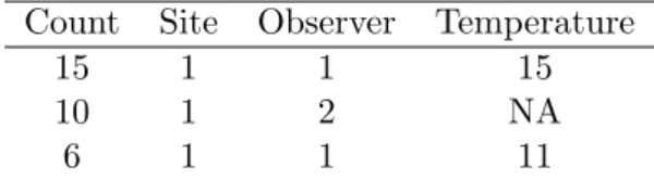
Table 1: Survey dataset for some wildlife species.

the analysis. However, this results in loss of information if an excluded observation contains valid values for other quantities, and can bias results. An alternative is to impute the missing values, based on information in the rest of the model.

For example, consider a survey dataset for some wildlife species in Table1. Each row contains the number of individuals seen during the survey, along with three covariates: the site on which the survey was conducted, the observer that collected the data, and the temperature during the survey. If we are interested in modelling, say, population size as a function of the count and the associated covariates, it is difficult to accommodate the second observation because the temperature is missing (perhaps the thermometer was broken that day). Ignoring this observation will allow us to fit the model, but it wastes information that is contained in the other covariates.

In a Bayesian modelling framework, missing data are accommodated simply by treating them as unknown model parameters. Values for the missing data ˜y are estimated naturally, using the posterior predictive distribution:

p(˜y|y) = Z

p(˜y|θ)f(θ|y)dθ (2) This describes additional data ˜y, which may either be considered unobserved data or potential future observations. We can use the posterior predictive distribution to model the likely values of missing data, which accounts for both predictive and inferential uncertainty.

Consider the coal mining disasters data introduced previously. Assume that two years of data are missing from the time series; we indicate this in the data array by the use of an arbitrary placeholder value,None.

x = numpy.array([ 4, 5, 4, 0, 1, 4, 3, 4, 0, 6, 3, 3, 4, 0, 2, 6, 3, 3, 5, 4, 5, 3, 1, 4, 4, 1, 5, 5, 3, 4, 2, 5, 2, 2, 3, 4, 2, 1, 3, None, 2, 1, 1, 1, 1, 3, 0, 0, 1, 0, 1, 1, 0, 0, 3, 1, 0, 3, 2, 2, 0, 1, 1, 1, 0, 1, 0, 1, 0, 0, 0, 2, 1, 0, 0, 0, 1, 1, 0, 2, 3, 3, 1, None, 2, 1, 1, 1, 1, 2, 4, 2, 0, 0, 1, 4, 0, 0, 0, 1, 0, 0, 0, 0, 0, 1, 0, 0, 1, 0, 1])

To estimate these values inPyMC, we generate a masked array. These are specialisedNumPy arrays that contain a matching TrueorFalsevalue for each element to indicate if that value should be excluded from any computation. Masked arrays can be generated using NumPy’s ma.masked_equal function:

>>> masked_data = numpy.ma.masked_equal(x, value=None) >>> masked_data

masked_array(data = [4 5 4 0 1 4 3 4 0 6 3 3 4 0 2 6 3 3 5 4 5 3 1 4 4 1 5 5 3 4 2 5 2 2 3 4 2 1 3 -- 2 1 1 1 1 3 0 0 1 0 1 1 0 0 3 1 0 3 2 2 0 1 1 1 0 1 0 1 0 0 0 2 1 0 0 0 1 1 0 2 3 3 1 -- 2 1 1 1 1 2 4 2 0 0 1 4 0 0 0 1 0 0 0 0 0 1 0 0 1 0 1],

mask = [False False False False False False False False False False False False False False False False False False False False False False False False False False False False False False False False False False False False False False False True False False False False False False False False False False False False False False False False False False False False False False False False False False False False False False False False False False False False False False False False False False False True False False False False False False False False False False False False False False False False False False False False False False False False False False False],

fill_value=?)

This masked array, in turn, can then be passed to PyMC’s own Impute function, which replaces the missing values with Stochastic variables of the desired type. For the coal mining disasters problem, recall that disaster events were modelled as Poisson variates:

>>> from pymc import Impute

>>> D = Impute('D', Poisson, masked_data, mu=r) >>> D [<pymc.distributions.Poisson 'D[0]' at 0x4ba42d0>, <pymc.distributions.Poisson 'D[1]' at 0x4ba4330>, <pymc.distributions.Poisson 'D[2]' at 0x4ba44d0>, <pymc.distributions.Poisson 'D[3]' at 0x4ba45f0>, ... <pymc.distributions.Poisson 'D[110]' at 0x4ba46d0>]

Here r is an array of means for each year of data, allocated according to the location of the switchpoint. Each element in D is a Poisson Stochastic, irrespective of whether the obser-vation was missing or not. The difference is that actual obserobser-vations are data Stochastics (observed=True), while the missing values are non-data Stochastics. The latter are consid-ered unknown, rather than fixed, and therefore estimated by the MCMC algorithm, just as unknown model parameters.

In this example, we have manually generated the masked array for illustration. In practice, theImputefunction will mask arrays automatically, replacing allNonevalues with Stochastics. Hence, only the original data array needs to be passed.

The entire model looks very similar to the original model:

s = DiscreteUniform('s', lower=0, upper=110) e = Exponential('e', beta=1)

l = Exponential('l', beta=1) @deterministic(plot=False)

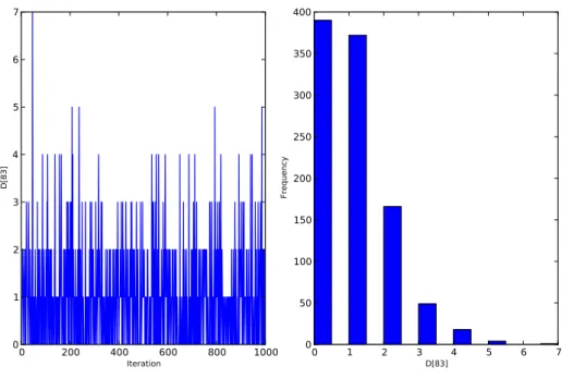
0 200 400 600 800 1000 Iteration 0 1 2 3 4 5 6 7 D[83] 0 1 2 3 4 5 6 7 D[83] 0 50 100 150 200 250 300 350 400 Frequency

Figure 5: Trace and posterior distribution of the second missing data point in the example.

def r(s=s, e=e, l=l):

"""Allocate appropriate mean to time series""" out = numpy.empty(len(disasters_array))

out[:s] = e out[s:] = l return out

D = Impute('D', Poisson, x, mu=r)

The main limitation of this approach for imputation is performance. Because each element in the data array is modelled by an individual Stochastic, rather than a single Stochastic for the entire array, the number of nodes in the overall model increases from 4 to 113. This significantly slows the rate of sampling, due to the overhead costs associated with iterations over individual nodes.

3.12. Fine-tuning the MCMC algorithm

MCMC objects handle individual variables viastep methods, which determine how parameters are updated at each step of the MCMC algorithm. By default, step methods are automat-ically assigned to variables by PyMC. To see which step methods M is using, look at its step_method_dictattribute with respect to each parameter:

>>> M.step_method_dict[DisasterModel.s]

>>> M.step_method_dict[DisasterModel.e]

[<pymc.StepMethods.Metropolis object at 0x3e8cbb0>] >>> M.step_method_dict[DisasterModel.l]

[<pymc.StepMethods.Metropolis object at 0x3e8ccb0>]

The value of step_method_dict corresponding to a particular variable is a list of the step methodsM is using to handle that variable.

You can forceM to use a particular step method by callingM.use_step_methodbefore telling it to sample. The following call will causeM to handle l with a standard Metropolis step method, but with proposal standard deviation equal to 2:

>>> from pymc import Metropolis

M.use_step_method(Metropolis, DisasterModel.l, proposal_sd=2.)

Another step method class, AdaptiveMetropolis, is better at handling highly-correlated variables. If your model mixes poorly, usingAdaptiveMetropolis is a sensible first thing to try.

3.13. Beyond the basics

That was a brief introduction to basic PyMC usage. Many more topics are covered in the subsequent sections, including:

ˆ ClassPotential, another building block for probability models in addition toStochastic and Deterministic

ˆ Normal approximations

ˆ Using custom probability distributions

ˆ Object architecture

ˆ Saving traces to the disk, or streaming them to the disk during sampling

ˆ Writing your own step methods and fitting algorithms.

Also, be sure to check out the documentation for the Gaussian process extension, which is available onPyMC’s download page athttp://code.google.com/p/pymc/downloads/list.

4. Building models

Bayesian inference begins with specification of a probability model relating unknown variables to data. PyMC provides three basic building blocks for probability models: Stochastic, Deterministicand Potential.

A Stochastic object represents a variable whose value is not completely determined by its parents, and a Deterministic object represents a variable that is entirely determined by its

parents. Stochastic and Deterministic are subclasses of the Variable class, which only serves as a template for other classes and is never actually implemented in models.

The third basic class, Potential, represents ‘factor potentials’ (Lauritzen, Dawid, Larsen, and Leimer 1990;Jordan 2004), which are not variables but simply terms and/or constraints that are multiplied into joint distributions to modify them. Potential and Variable are subclasses ofNode.

PyMC probability models are simply linked groups of Stochastic, Deterministic and Potential objects. These objects have very limited awareness of the models in which they are embedded and do not themselves possess methods for updating their values in fitting algorithms. Objects responsible for fitting probability models are described in Section5.

4.1. The Stochastic class

A stochastic variable has the following primary attributes:

value: The variable’s current value.

logp: The log-probability of the variable’s current value given the values of its parents.

A stochastic variable can optionally be endowed with a method called rand, which draws a value for the variable given the values of its parents2. Stochastic variables have the following additional attributes:

parents: A dictionary containing the variable’s parents. The keys of the dictionary are to the labels assigned to the parents by the variable, and the values correspond to the actual parents. For example, the keys of s’s parents dictionary in model (1) would be ‘t_l’ and‘t_h’. The actual parents (i.e., the values of the dictionary) may be of any class or type.

children: A set containing the variable’s children.

extended_parents: A set containing all stochastic variables on which the variable depends, either directly or via a sequence of deterministic variables. If the value of any of these variables changes, the variable will need to recompute its log-probability.

extended_children: A set containing all stochastic variables and potentials that depend on the variable, either directly or via a sequence of deterministic variables. If the variable’s value changes, all of these variables and potentials will need to recompute their log-probabilities.

observed: A flag (boolean) indicating whether the variable’s value has been observed (is fixed).

dtype: A NumPy dtype object (such asnumpy.int) that specifies the type of the variable’s value. The variable’s value is always cast to this type. If this is None (default) then no type is enforced.

4.2. Creation of stochastic variables

There are three main ways to create stochastic variables, called theautomatic,decorator, and direct interfaces.

Automatic Stochastic variables with standard distributions provided by PyMC (see

Ap-pendix) can be created in a single line using special subclasses of Stochastic. For example, the uniformly-distributed discrete variable sin (1) could be created using the automatic interface as follows:

import pymc as pm

s = pm.DiscreteUniform('s', 1851, 1962, value=1900)

In addition to the classes in the appendix,scipy.stats.distributions’ random vari-able classes are wrapped asStochasticsubclasses ifSciPyis installed. These distribu-tions are in the submodule pymc.SciPyDistributions.

Users can call the class factory stochastic_from_dist to produce Stochastic sub-classes of their own from probability distributions not included with PyMC.

Decorator Uniformly-distributed discrete stochastic variablesin (1) could alternatively be

created from a function that computes its log-probability as follows:

@pm.stochastic(dtype=int)

def s(value=1900, t_l=1851, t_h=1962):

"""The switchpoint for the rate of disaster occurrence.""" if value > t_h or value < t_l:

return -numpy.inf else:

return -numpy.log(t_h - t_l + 1)

Note that this is a simple Python function preceded by a Python expression called a decorator (van Rossum 2010), here called@stochastic. Generally, decorators enhance functions with additional properties or functionality. The Stochasticobject produced by the @stochastic decorator will evaluate its log-probability using the function s. The value argument, which is required, provides an initial value for the variable. The remaining arguments will be assigned as parents ofs(i.e., they will populate theparents dictionary).

To emphasize, the Pythonfunction decorated by @stochasticshould compute the log -density or log-probability of the variable. That’s why the return value in the example above is −log(th−tl+ 1) rather than 1/(th−tl+ 1).

The value and parents of stochastic variables may be any objects, provided the log-probability function returns a real number (float). PyMC and SciPy both provide implementations of several standard probability distributions that may be helpful for creating custom stochastic variables. Based on informal comparison using version 2.0, the distributions inPyMCtend to be approximately an order of magnitude faster than their counterparts inSciPy(using version 0.7). See thePyMCwiki page on benchmarks athttp://code.google.com/p/pymc/wiki/Benchmarks.

The decorator stochasticcan take any of the argumentsStochastic.__init__takes except parents,logp,random,docand value. These arguments includetrace,plot, verbose,dtype,rseed andname.

The decorator interface has a slightly more complex implementation which allows you to specify a random method for sampling the stochastic variable’s value conditional on its parents.

@pm.stochastic(dtype=int)

def s(value=1900, t_l=1851, t_h=1962):

"""The switchpoint for the rate of disaster occurrence.""" def logp(value, t_l, t_h): if value > t_h or value < t_l: return -numpy.inf else: return -numpy.log(t_h - t_l + 1) def random(t_l, t_h):

return numpy.round( (t_l - t_h) * random() ) + t_l

The stochastic variable again gets its name, docstring and parents from functions, but in this case it will evaluate its log-probability using the logp function. The random function will be used when s.random() is called. Note that random doesn’t take a value argument, as it generates values itself.

Direct It’s possible to instantiate Stochasticdirectly:

def s_logp(value, t_l, t_h): if value > t_h or value < t_l: return -numpy.inf else: return -numpy.log(t_h - t_l + 1) def s_rand(t_l, t_h):

return numpy.round( (t_l - t_h) * random() ) + t_l s = pm.Stochastic( logp = s_logp,

doc = 'The switchpoint for the rate of disaster occurrence.', name = 's', parents = {`t_l': 1851, 't_h': 1962}, random = s_rand, trace = True, value = 1900, dtype=int, rseed = 1., observed = False, cache_depth = 2,

plot=True, verbose = 0)

Notice that the log-probability and random variate functions are specified externally and passed to Stochastic as arguments. This is a rather awkward way to instantiate a stochastic variable; consequently, such implementations should be rare.

4.3. A warning: Don’t update stochastic variables’ values in-place

Stochasticobjects’ values should not be updated in-place. This confuses PyMC’s caching scheme and corrupts the process used for accepting or rejecting proposed values in the MCMC algorithm. The only way a stochastic variable’s value should be updated is using statements of the following form:

A.value = new_value

The following are in-place updates and shouldnever be used:

ˆ A.value += 3

ˆ A.value[2,1] = 5

ˆ A.value.attribute = new_attribute_value.

This restriction becomes onerous if a step method proposes values for the elements of an array-valued variable separately. In this case, it may be preferable to partition the variable into several scalar-valued variables stored in an array or list.

4.4. Data

Data are represented by Stochastic objects whose observed attribute is set to True. Al-though the data are modelled with statistical distributions, their values should be treated as immutable (since they have been observed). If a stochastic variable’sobservedflag is True, its value cannot be changed, and it won’t be sampled by the fitting method.

4.5. Declaring stochastic variables to be data

In each interface, an optional keyword argumentobservedcan be set toTrue. In the decorator interface, this argument is added to the@stochastic decorator:

@pm.stochastic(observed=True)

In the other interfaces, theobserved=Trueargument is added to the initialization arguments:

x = pm.Binomial('x', value=7, n=10, p=.8, observed=True)

Alternatively, in the decorator interface only, aStochasticobject’sobservedflag can be set to true by using an@observed decorator in place of the@stochastic decorator:

@observed(dtype=int) def ...

4.6. The Deterministic class

TheDeterministicclass represents variables whose values are completely determined by the values of their parents. For example, in model (1),r is a deterministic variable. Recall it was defined by

rt=

e t≤s l t > s ,

sor’s value can be computed exactly from the values of its parents e,l and s.

Adeterministicvariable’s most important attribute isvalue, which gives the current value of the variable given the values of its parents. LikeStochastic’slogpattribute, this attribute is computed on-demand and cached for efficiency.

A Deterministic variable has the following additional attributes:

parents: A dictionary containing the variable’s parents. The keys of the dictionary corre-spond to the labels assigned to the parents, and the values correcorre-spond to the actual parents.

children: A set containing the variable’s children, which must be nodes (variables or poten-tials).

Deterministic variables have no methods.

4.7. Creation of deterministic variables

There are several ways to create deterministic variables:

Automatic A handful of common functions have been wrapped in Deterministic subclasses.

These are brief enough to list:

LinearCombination: Has two parents x and y, both of which must be iterable (i.e., vector-valued). The value of a linear combination is

X

i

xT_i yi.

Index: Has two parentsx and index. xmust be iterable, indexmust be valued as an integer. The value of an index is

x[index].

Index is useful for implementing dynamic models, in which the parent-child con-nections change.

Lambda: Converts an anonymous function (in Python, called lambda functions) to a Deterministic instance on a single line.

CompletedDirichlet: PyMCrepresents Dirichlet variables of lengthkby the firstk−1 elements; since they must sum to 1, thek−th element is determined by the others. CompletedDirichlet appends thek−th element to the value of its parent D. Logit, InvLogit, StukelLogit, StukelInvLogit: Two common link functions for

gen-eralized linear models and their inverses.

It’s a good idea to use these classes when feasible in order to give hints to step methods.

Elementary operations on variables Certain elementary operations on variables create

deterministic variables. For example:

>>> x = pm.MvNormalCov('x',numpy.ones(3),numpy.eye(3)) >>> y = pm.MvNormalCov('y',numpy.ones(3),numpy.eye(3)) >>> print x+y <pymc.PyMCObjects.Deterministic '(x_add_y)' at 0x105c3bd10> >>> print x[0] <pymc.CommonDeterministics.Index 'x[0]' at 0x105c52390> >>> print x[1]+y[2] <pymc.PyMCObjects.Deterministic '(x[1]_add_y[2])' at 0x105c52410>

All the objects thus created havetrace=Falseandplot=Falseby default. This conve-nient method of generating simple deterministics was inspired by Kerman and Gelman

(2004).

Decorator A deterministic variable can be created via a decorator in a way very similar to

Stochastic’s decorator interface:

@pm.deterministic

def r(switchpoint = s, early_rate = e, late_rate = l): """The rate of disaster occurrence."""

value = numpy.zeros(len(D)) value[:switchpoint] = early_rate value[switchpoint:] = late_rate return value

Notice that rather than returning the log-probability, as is the case for Stochastic objects, the function returns the value of the deterministic object, given its parents. This return value may be of any type, as is suitable for the problem at hand. Also notice that, unlike for Stochastic objects, there is no value argument passed, since the value is calculated deterministically by the function itself. Arguments’ keys and values are converted into a parent dictionary as with Stochastic’s short interface. The deterministic decorator can taketrace, verbose and plot arguments, like the stochastic decorator3.

Direct Deterministic can also be instantiated directly:

3

Note that deterministic variables have no observedflag. If a deterministic variable’s value were known, its parents would be restricted to the inverse image of that value under the deterministic variable’s evaluation function. This usage would be extremely difficult to support in general, but it can be implemented for particular applications at theStepMethodlevel.

def r_eval(switchpoint = s, early_rate = e, late_rate = l): value = numpy.zeros(len(D)) value[:switchpoint] = early_rate value[switchpoint:] = late_rate return value r = pm.Deterministic(eval = r_eval, name = 'r',

parents = {`switchpoint': s, 'early_rate': e, 'late_rate': l}, doc = 'The rate of disaster occurrence.',

trace = True, verbose = 0, dtype=float, plot=False, cache_depth = 2) 4.8. Containers

In some situations it would be inconvenient to assign a unique label to each parent of a variable. Considery in the following model:

x0∼N(0, τx) xi+1|xi∼N(xi, τx) i= 0, . . . , N−2 y|x∼N N−1 X i=0 x2_i, τy !

Here,y depends on every element of the Markov chainx, but we wouldn’t want to manually enterN parent labels ‘x_0’,‘x_1’, etc.

This situation can be handled easily inPyMC:

N = 10

x_0 = pm.Normal('x_0', mu=0, tau=1) x = numpy.empty(N, dtype=object) x[0] = x_0

for i in range(1,N):

x[i] = pm.Normal('x_%i' % i, mu=x[i-1], tau=1) @pm.observed

def y(value = 1, mu = x, tau = 100):

return pm.normal_like(value, numpy.sum(mu**2), tau)

PyMC automatically wraps array x in an appropriate Container class. The expression ‘x_%i’%i labels each Normal object in the container with the appropriate index i; so if i=1, the name of the corresponding element becomes‘x_1’.

Containers, like variables, have an attribute calledvalue. This attribute returns a copy of the (possibly nested) iterable that was passed into the container function, but with each variable inside replaced with its corresponding value.

Containers can currently be constructed from lists, tuples, dictionaries, Numpy arrays, mod-ules, sets or any object with a__dict__attribute. Variables and non-variables can be freely mixed in these containers, and different types of containers can be nested4. Containers at-tempt to behave like the objects they wrap. All containers are subclasses ofContainerBase. Containers have the following useful attributes in addition tovalue:

ˆ variables ˆ stochastics ˆ potentials ˆ deterministics ˆ data_stochastics ˆ step_methods.

Each of these attributes is a set containing all the objects of each type in a container, and within any containers in the container.

4.9. The Potential class

The joint density corresponding to model (1) can be written as follows:

p(D, s, l, e) =p(D|s, l, e)p(s)p(l)p(e).

Each factor in the joint distribution is a proper, normalized probability distribution for one of the variables conditional on its parents. Such factors are contributed byStochasticobjects. In some cases, it’s nice to be able to modify the joint density by incorporating terms that don’t correspond to probabilities of variables conditional on parents, for example:

p(x0, x2, . . . xN−1)∝

N−2 Y

i=0

ψi(xi, xi+1).

In other cases we may want to add probability terms to existing models. For example, suppose we want to constrain the difference betweeneand l in (1) to be less than 1, so that the joint density becomes

p(D, s, l, e)∝p(D|s, l, e)p(s)p(l)p(e)I(|e−l|<1).

It’s possible to express this constraint by adding variables to the model, or by groupingeand

lto form a vector-valued variable, but it’s uncomfortable to do so.

4

Nodes whose parents are containers make private shallow copies of those containers. This is done for technical reasons rather than to protect users from accidental misuse.

Arbitrary factors such as ψ and the indicator function I(|e−l| < 1) are implemented by objects of classPotential(Lauritzenet al.(1990) andJordan(2004) call these terms ‘factor potentials’). Bayesian hierarchical notation (cf model (1)) doesn’t accomodate these poten-tials. They are often used in cases where there is no natural dependence hierarchy, such as the first example above (which is known as a Markov random field). They are also useful for expressing ‘soft data’ (Christakos 2002) as in the second example above.

Potentials have one important attribute,logp, the log of their current probability or proba-bility density value given the values of their parents. The only other attribute of interest is parents, a dictionary containing the potential’s parents. Potentials have no methods. They have no trace attribute, because they are not variables. They cannot serve as parents of variables (for the same reason), so they have nochildrenattribute.

4.10. An example of soft data

The role of potentials can be confusing, so we will provide another example: we have a dataset

t consisting of the days on which several marked animals were recaptured. We believe that the probability S that an animal is not recaptured on any given day can be explained by a covariate vectorx. We model this situation as follows:

ti|Si ∼ Geometric(Si), i= 1. . . N

Si = logit−1(βxi)

β ∼ N(µβ, Vβ).

So far, so good. Now suppose we have some knowledge of other related experiments and we are confidentS will be independent of the value of β. It’s not obvious how to work this ‘soft data’, because as we’ve written the modelS is completely determined by β. There are three options within the strict Bayesian hierarchical framework:

ˆ Work the soft data into the prior onβ.

ˆ Incorporate the data from the previous experiments explicitly into the model.

ˆ Refactor the model so that S is at the bottom of the hierarchy, and assign the prior directly.

Factor potentials provide a convenient way to incorporate the soft data without the need for such major modifications. We can simply modify the joint distribution from

p(t|S(x, β))p(β) to

γ(S)p(t|S(x, β))p(β),

where the value ofγ is large ifS’s value is plausible (based on our external information) and small otherwise. We do not know the normalizing constant for the new distribution, but we don’t need it to use most popular fitting algorithms. It’s a good idea to check the induced

priors onS and β for sanity. This can be done inPyMC by fitting the model with the data

tremoved.

It’s important to understand thatγ is not a variable, so it does not have a value. That means, among other things, there will be noγ column in MCMC traces.

4.11. Creation of Potentials There are two ways to create potentials:

Decorator A potential can be created via a decorator in a way very similar toDeterministic’s

decorator interface:

@pm.potential

def psi_i(x_lo = x[i], x_hi = x[i+1]): """A pair potential"""

return -(x_lo - x_hi)**2

The function supplied should return the potential’s currentlog-probability orlog-density as a NumPy float. The potential decorator can take verbose and cache_depth arguments like the stochasticdecorator.

Direct The same potential could be created directly as follows:

def psi_i_logp(x_lo = x[i], x_hi = x[i+1]): return -(x_lo - x_hi)**2

psi_i = pm.Potential( logp = psi_i_logp, name = 'psi_i',

parents = {`xlo': x[i], 'xhi': x[i+1]}, doc = 'A pair potential',

verbose = 0, cache_depth = 2)

4.12. Graphing models

The function graph (or dag) in pymc.graph draws graphical representations of Model (Sec-tion 5) instances usingGraphviz via thePython package PyDot. See Lauritzen et al. (1990) and Jordan (2004) for more discussion of useful information that can be read off of graphical models. Note that these authors do not consider deterministic variables.

The symbol for stochastic variables is an ellipse. Parent-child relationships are indicated by arrows. These arrows point from parent to child and are labeled with the names assigned to the parents by the children. PyMC’s symbol for deterministic variables is a downward-pointing triangle. A graphical representation of model (1) is shown in Figure2. Note thatD

is shaded because it is flagged as data.

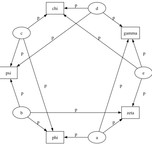
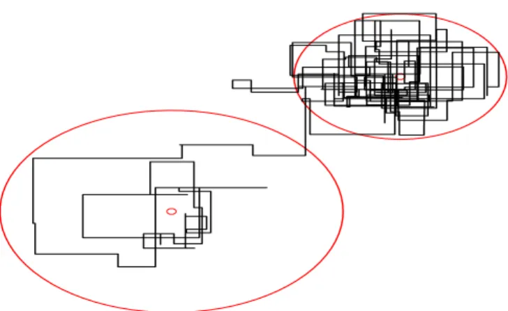
The symbol for factor potentials is a rectangle (Figure 6). Factor potentials are usually as-sociated with undirected grahical models. In undirected representations, each parent of a potential is connected to every other parent by an undirected edge. The undirected represen-tation of the model is much more compact (Figure 7). Directed or mixed graphical models

a phi p zeta p gamma p c chi p p psi p b p p p e p p p d p p p

Figure 6: Directed graphical model example. Factor potentials are represented by rectangles and stochastic variables by ellipses.

can be represented in an undirected form by ‘moralizing’, which is done by the function pymc.graph.moral_graph.

4.13. Class LazyFunction and caching

This section gives an overview of how PyMC computes log-probabilities. This is advanced information that is not required in order to use PyMC.

The logp attributes of stochastic variables and potentials and the value attributes of de-terministic variables are wrappers for instances of class LazyFunction. Lazy functions are wrappers for ordinaryPython functions. A lazy functionL could be created from a function fun as follows:

L = pm.LazyFunction(fun, arguments)

The argumentargumentsis a dictionary container;funmust accept keyword arguments only. WhenL’sget() method is called, the return value is the same as the call

fun(**arguments.value)

a

c

b

e

d

Figure 7: The undirected version of the graphical model of Figure6.

Before calling fun, L will check the values of its arguments’ extended children against an internal cache. This comparison is done by reference, not by value, and this is part of the reason why stochastic variables’ values cannot be updated in-place. If the arguments’ extended children’s values match a frame of the cache, the corresponding output value is returned and funis not called. If a call tofunis needed, the arguments’ extended children’s values and the return value replace the oldest frame in the cache. The depth of the cache can be set using the optional init argumentcache_depth, which defaults to 2.

Caching is helpful in MCMC, because variables’ log-probabilities and values tend to be queried multiple times for the same parental value configuration. The default cache depth of 2 turns out to be most useful in Metropolis-Hastings-type algorithms involving proposed values that may be rejected.

Lazy functions are implemented inCusingPyrex(Ewing 2010), a language for writingPython extensions.

5. Fitting models

PyMC provides three objects that fit models:

ˆ MCMC, which coordinates Markov chain Monte Carlo algorithms. The actual work of updating stochastic variables conditional on the rest of the model is done byStepMethod objects, which are described in this section.

ˆ MAP, which computes maximum a posteriori estimates.

ˆ NormApprox, which computes the ‘normal approximation’ (Gelman et al. 2004): the joint distribution of all stochastic variables in a model is approximated as normal using local information at the maximum a posteriori estimate.

All three objects are subclasses of Model, which is PyMC’s base class for fitting methods. MCMCand NormApprox, both of which can produce samples from the posterior, are subclasses ofSampler, which is PyMC’s base class for Monte Carlo fitting methods. Sampler provides a generic sampling loop method and database support for storing large sets of joint samples. These base classes are documented at the end of this section.

5.1. Creating models

The first argument to any fitting method’s init method, including that of MCMC, is called input. The input argument can be just about anything; once you have defined the nodes that make up your model, you shouldn’t even have to think about how to wrap them in a Modelinstance. Some examples of model instantiation using nodes a,band cfollow:

ˆ M = Model(set([a,b,c]))

ˆ M = Model({‘a’: a, ‘d’: [b,c]}) In this case, M will expose a and d as at-tributes: M.awill bea, andM.d will be[b,c].

ˆ M = Model([[a,b],c])

ˆ If file MyModulecontains the definitions ofa,bandc:

import MyModule M = Model(MyModule)

In this case, M will expose a,b andc as attributes.

ˆ Using a ‘model factory’ function:

def make_model(x): a = pm.Exponential('a',beta=x,value=0.5) @pm.deterministic def b(a=a): return 100-a @pm.stochastic

def c(value=0.5, a=a, b=b): return (value-a)**2/b return locals()

M = pm.Model(make_model(3))

In this case, M will also exposea,band c as attributes. 5.2. The Model class

Modelserves as a container for probability models and as a base class for the classes responsible for model fitting, such asMCMC.

input: Some collection of PyMC nodes defining a probability model. These may be stored in a list, set, tuple, dictionary, array, module, or any object with a __dict__attribute.

verbose (optional): An integer controlling the verbosity of the model’s output.

Models’ useful methods are:

draw_from_prior(): Sets all stochastic variables’ values to new random values, which would be a sample from the joint distribution if all data andPotentialinstances’ log-probability functions returned zero. If any stochastic variables lack arandom()method,PyMCwill raise an exception.

seed(): Same as draw_from_prior, but only stochastics whose rseed attribute is not None are changed.

The helper functiongraphproduces graphical representations of models (Jordan 2004, see). Models have the following important attributes:

ˆ variables ˆ stochastics ˆ potentials ˆ deterministics ˆ observed_stochastics ˆ step_methods

ˆ value: A copy of the model, with each attribute that is a PyMC variable or container replaced by its value.

ˆ generations: A topological sorting of the stochastics in the model.

In addition, models expose each node they contain as an attribute. For instance, if modelM were produced from model (1) M.swould return the switchpoint variable.

5.3. Maximum a posteriori estimates

The MAP class sets all stochastic variables to their maximuma posteriori values using func-tions in SciPy’s optimize package. SciPy must be installed to use it. MAP can only han-dle variables whose dtype is float, so it will not work on model 1. To fit the model in examples/gelman_bioassay.pyusing MAP, do the following

>>> from pymc.examples import gelman_bioassay >>> M = pm.MAP(gelman_bioassay)

>>> M.fit()

This call will cause M to fit the model using Nelder-Mead optimization, which does not require derivatives. The variables ingelman_bioassayhave now been set to their maximum a posteriori values:

>>> M.alpha.value

array(0.8465892309923545) >>> M.beta.value

array(7.7488499785334168)

In addition, the AIC and BIC of the model are now available:

>>> M.AIC

7.9648372671389458 >>> M.BIC

6.7374259893787265

MAPhas two useful methods:

fit(method =’fmin’, iterlim=1000, tol=.0001): The optimization method may befmin, fmin_l_bfgs_b,fmin_ncg,fmin_cg, orfmin_powell. See the documentation ofSciPy’s optimize package for the details of these methods. The tol and iterlim parameters are passed to the optimization function under the appropriate names.

revert_to_max(): If the values of the constituent stochastic variables change after fitting, this function will reset them to their maximuma posteriori values.

If you’re going to use an optimization method that requires derivatives, MAP’s init method can take additional parametersepsanddiff_order. diff_order, which must be an integer, specifies the order of the numerical approximation (see theSciPyfunctionderivative). The step size for numerical derivatives is controlled byeps, which may be either a single value or a dictionary of values whose keys are variables (actual objects, not names).

The useful attributes ofMAPare:

logp: The joint log-probability of the model.

logp_at_max: The maximum joint log-probability of the model.

AIC: Akaike’s information criterion for this model (Akaike 1973; Burnham and Anderson 2002).

BIC: The Bayesian information criterion for this model (Schwarz 1978).

One use of the MAP class is finding reasonable initial states for MCMC chains. Note that multiple Modelsubclasses can handle the same collection of nodes.

5.4. Normal approximations

The NormApproxclass extends theMAPclass by approximating the posterior covariance of the model using the Fisher information matrix, or the Hessian of the joint log probability at the maximum. To fit the model inexamples/gelman_bioassay.pyusing NormApprox, do:

>>> N = pm.NormApprox(gelman_bioassay) >>> N.fit()

The approximate joint posterior mean and covariance of the variables are available via the attributesmu andC: >>> N.mu[N.alpha] array([ 0.84658923]) >>> N.mu[N.alpha, N.beta] array([ 0.84658923, 7.74884998]) >>> N.C[N.alpha] matrix([[ 1.03854093]]) >>> N.C[N.alpha, N.beta] matrix([[ 1.03854093, 3.54601911], [ 3.54601911, 23.74406919]])

As with MAP, the variables have been set to their maximum a posteriori values (which are also in themuattribute) and the AIC and BIC of the model are available.

In addition, it’s now possible to generate samples from the posterior as withMCMC:

>>> N.sample(100) >>> N.trace('alpha')[::10] array([-0.85001278, 1.58982854, 1.0388088 , 0.07626688, 1.15359581, -0.25211939, 1.39264616, 0.22551586, 2.69729987, 1.21722872]) >>> N.trace('beta')[::10] array([ 2.50203663, 14.73815047, 11.32166303, 0.43115426, 10.1182532 , 7.4063525 , 11.58584317, 8.99331152, 11.04720439, 9.5084239 ])

Any of the database backends can be used (Section 6).

In addition to the methods and attributes ofMAP,NormApproxprovides the following methods:

sample(iter): Samples from the approximate posterior distribution are drawn and stored.

isample(iter): An ‘interactive’ version of sample(): sampling can be paused, returning control to the user.

draw: Sets all variables to random values drawn from the approximate posterior.

It provides the following additional attributes:

mu: A special dictionary-like object that can be keyed with multiple variables. N.mu[p1, p2, p3] would return the approximate posterior mean values of stochastic variables p1,p2 and p3, ravelled and concatenated to form a vector.

C: Another special dictionary-like object. N.C[p1, p2, p3] would return the approximate posterior covariance matrix of stochastic variables p1, p2 and p3. As with mu, these variables’ values are ravelled and concatenated before their covariance matrix is con-structed.