A generalized additive model approach to
time-to-event analysis
Andreas Bender1, Andreas Groll2and Fabian Scheipl1
1Department of Statistics, Ludwig-Maximilians-Universit ¨at, M ¨unchen, Germany. 2Chairs of Statistics and Econometrics, Georg-August-Universit ¨at G ¨ottingen, Germany.
Abstract: This tutorial article demonstrates how time-to-event data can be modelled in a very flexible way by taking advantage of advanced inference methods that have recently been developed for generalized additive mixed models. In particular, we describe the necessary pre-processing steps for transforming such data into a suitable format and show how a variety of effects, including a smooth nonlinear baseline hazard, and potentially nonlinear and nonlinearly time-varying effects, can be estimated and interpreted. We also present useful graphical tools for model evaluation and interpretation of the estimated effects. Throughout, we demonstrate this approach using various application examples. The article is accompanied by a newR-package calledpammtoolsimplementing all of the tools described here.
Key words: Cox model, time-varying coefficients, piece-wise exponential model, penalization, survival analysis, splines
RecievedMay 2017;revisedSeptember 2017;acceptedSeptember 2017
1 Introduction
In this tutorial, we introduce a general framework for fitting time-to-event data, that is, the time until an event occurs, denoted by (the random variable) T. Classical application examples, which we will discuss in more detail later, include time until death of cancer patients and time until convicts are rearrested. When modelling such data, the central property of interest is usually the survival functionS(t) :=P(T > t), that is, the probability for an event occurring after time t. The modelling of such data, however, generally focuses on the so-called hazard rate, in the following denoted by (t), which represents the instantaneous (normalized) risk of having an event in t, given no event occurred up to time t. The corresponding mathematical, rather technical definition of the hazard rate, is given as follows:
(t) := lim
t→0
P(t ≤T < t+t|T ≥t)
t . (1.1)
Address for correspondence: Andreas Groll, Chairs of Statistics and Econometrics, Georg-August-Universit ¨at, Humboldtallee 3, 37073 G ¨ottingen, Germany.
E-mail: [email protected]
In the following, we demonstrate how a large class of models for time-to-event data can be represented as generalized additive mixed models (GAMMs). Using this representation, which requires a specific transformation of the original time-to-event data (see Section 2.2 for details), all the methods and versatile software imple-mentations available for GAMMs, many of which are covered in this special issue, can be applied to survival analysis. In this way, the specification and penalized estimation of, for example, nonlinear, spatial or random effects for time-to-event data becomes routine and rather easy to do, equally so for (nonlinearly) time-varying effects.
The representation described here is not novel and known in the literature as piece-wise exponential models (PEMs). Under certain assumptions, PEMs are essentially Poisson generalized linear models (GLMs; Holford, 1980; Laird and Olivier, 1981; Friedman, 1982) with likelihoods proportional to the (partial) likelihood of a corresponding Cox model (see Cox, 1972 and Equation (2.1)). The PEM representation was popular temporarily when implementations of GLMs were more readily available in different statistical software packages compared to implementations of dedicated algorithms for survival models (Whitehead, 1980; Clayton, 1983), but most research in the field of survival analysis has concentrated on the Cox model and its extensions or on models based on the counting process representation of time-to-event data (Andersen et al., 1992; Martinussen and Scheike, 2006).
The PEM representation requires a partition of the follow-up time into a finite number of intervals and assumes that hazard rates are piece-wise constant in each of these intervals. The arbitrary choice of cut-points defining this partition has often been a point of criticism regarding PEMs. If the number of cut-points is too small, the step function approximation of the hazard rate may be too crude. A large number of cut-points, on the other hand, may lead to over-fitting and inefficient estimation with unstable estimates, as the baseline hazard requires the estimation of one parameter per interval. We are convinced, however, that the usage of PEMs remains desirable, especially in situations where one wants to take advantage of the methodological (Wood, 2011) and algorithmic (Wood, 2017) advances that have been made for GAMMs over the last years, particularly whenever inclusion of nonlinear, multivariate, spatial or spatio-temporal, or random effects is required. Even more importantly, the current state of the art for additive models allows analysts to largely avoid the ‘arbitrary cut-points’ problem of classical PEMs. Analysts can simply use a large number of cut-points and estimate the baseline hazard and other time-varying effects semiparametrically, while avoiding over-fitting and instability by means of penalization. We call this extension of the PEM a Piece-wise exponential Additive Mixed Model (PAMM).
This idea has been utilized in many recent publications. For example, Rodr´ıguez-Girondo et al. (2013) use this approach to discuss model building strategies, including double shrinkage methods. Argyropoulos and Unruh (2015) discuss a variant of this method, which they call Poisson generalized additive model (GAM) using a Gauß–Lobato quadrature rule to partition the follow-up. They also give a thorough overview of methods for flexible parametric inference for time-to-event data as well as an overview of previous research on the Poisson
model for survival analysis. Sennhenn-Reulen and Kneib (2016) use PAMMs to fit LASSO-penalized multi-state models, while Gasparrini et al. (2017) extend distributed lag nonlinear models known from time-series analysis to the analysis of time-to-event data. Despite these recent publications and applications, the general idea of using GAMMs in the context of survival analysis is still not widely known by practitioners in substantive sciences, and the application of PAMMs is hindered by the lack of readily available clear-cut instructions on practical details such as data transformation and dedicated software that facilitate preparation and evaluation of such models.
Thus, the goal of this tutorial is to introduce and describe the general idea of the classical PEM as well as its semiparametric extension, the PAMM, and illustrate their use, starting from data transformation and standard models to more advanced applications. This tutorial is aimed at practitioners and focuses on building intuition and providing applicable advice rather than methodological detail and mathematical rigour. References for further reading are provided throughout. All results presented in this tutorial can be reproduced using the instructions and code in the vignettes of the add-on package pammtools (Bender and Scheipl, 2017), as described in Section 4.
In the following sections, we give a brief introduction to the PEM (Section 2) and its mathematical representation as a Poisson GLM (Section 2.1), as well as the data transformation required for its estimation (Section 2.2). We then describe the transition from PEMs to PAMMs in Section 2.3 and briefly outline the advantages of this approach. In Section 3, several examples for the application of PAMMs are provided, ranging from very simple (baseline hazard, time-constant effects) to more advanced models (stratified baseline hazards, nonlinearly time-varying effects, etc.).
2 Piece-wise exponential (additive) models
PEMs represent an alternative to classical approaches for continuous time-to-event data like, for example, the Cox model. If the partition of the follow-up time is selected with care, PEMs allow analysts to take advantage of all of the methodological and algorithmic advances that have been made for GAMMs over the last decades. In particular, it is fairly easy to include diverse types of effects such as nonlinear, multivariate, spatial, spatio-temporal or random effects in existing software packages for GAMMs.
Figure 1 illustrates the basic idea of a PEM for time-to-event data by applying it to survival times drawn from a Weibull distribution. To estimate the true underlying Weibull hazard rate (left panel), the follow-up is partitioned into a fixed number of intervals (here J=5) with interval cut-points 0=0<· · ·< J =4 (mid panel)
and a constant hazard is estimated for each interval (right panel). Thus, the name piece-wise exponential—the hazard rate of an exponential distribution is constant over time. The approximation in Figure 1 appears rather crude, but given enough cut-points, PEM and PAMM estimates are very similar (or even equivalent) to Cox regression estimates, as demonstrated in Section 3.
0.0 0.3 0.6 0.9 0.0 0.3 0.6 0.9 0.0 0.3 0.6 0.9 0 1 2 3 4 κ0=0κ1=0.8κ2=1.6κ3=2.4κ4=3.2κ5=4 κ0=0κ1=0.8κ2=1.6κ3=2.4κ4=3.2κ5=4 t t t λ ( t ) λ ( t ) λ ( t )
Figure 1 Hazard rate of a Weibull distribution (left panel); partitioning of the follow-up intoJ=5 intervals (mid panel); estimate of the hazard rate via interval-specific piece-wise constant hazards, obtained by fitting a PEM to the data (right panel)
The difference between a PEM and a PAMM then results from the different approaches for the estimation of the baseline hazard and other smooth, potentially time-varying effects. It is important to note that although PAMMs model the baseline hazard using a smooth, nonlinear function, the resulting (estimated) hazard rate is still piece-wise constant (see Section 2.3).
2.1 The Poisson-likelihood of a PEM
Following Bender et al. (2016), we now introduce PEMs more formally. We start with a general proportional hazards (PH) model given by
i(t|xi)=0(t) exp(xTiˇ), i= 1, . . . , n, (2.1)
wherenis the number of subjects under study,xi =(xi,1, . . . , xi,p)Tis the row vector
of time-constant covariates for subjecti, andˇthe vector of corresponding regression coefficients. In the framework of the Cox PH model, the parametersˇare estimated via partial likelihood, while the baseline hazard0(t) is estimated non-parametrically
via the Nelson–Aaalen estimator. A PEM is obtained by partitioning the follow-up period (0, tmax], where tmax denotes the maximal (observed) follow-up time, into
J intervals. To this end, we define J+1 cut-points 0=0< · · ·< J =tmax. The
j-th interval is then given by (j−1, j]. Assuming a constant hazard rate within each
intervalj, that is,0(t)= j∀t∈(j−1, j], t > 0, (2.1) simplifies to
i(t|xi)=jexp(xTiˇ), ∀t ∈(j−1, j]. (2.2)
If the underlying time-to-event data is structured in a certain way, that is, containing event indicatorsıij and offsetsoij for all intervalsjin which subjectiis under risk, it
E(ıij|xi)= exp(log(j)+xTiˇ+oij) (2.3)
is proportional to the one of model (2.2). Consequently, the two models are equivalent with respect to the ML estimator ofˇ. In practice, when fitting the respective Poisson GLM, log(j) is incorporated in the linear predictorxTiˇ, such that the design matrixX
containsJ additional dummy coded columns, where columnjtakes value 1 in rows representing observations in interval (j−1, j] and 0 otherwise. The oij are simply
added to the linear predictor as a so-called offset, which is usually of little interest, but note that the offset contains the information on the actual observed survival time in each interval, and thus makes the PEM a model for continuous time-to-event data, such that (2.3) can be reformulated asi(t|xi)= E(ıtij|xi)
ij =jexp(x
iˇ) (where
tij = exp(oij); cf. Section 2.2). For the remainder of the article, we will omit the offset
oij from the model specification, but it is important to stress that the offset must be
included at the estimation stage.
Note that if the survival time is in fact discrete, was only observed on a discrete grid or can be reasonably discretized without loss of information, most of the methods and strategies presented here are equally applicable to discrete-time models. These are described in detail in the tutorial by Berger and Schmid (2018), which is also part of this special issue.
In the next section, we illustrate how to transform time-to-event data to be in accordance with the model specification (2.3).
2.2 Data transformation
To fit the PEM introduced in the previous section, time-to-event data needs to be transformed and restructured in a specific way. First, for each subjectiletTidenote its
true survival time andCiits (non-informative) censoring time. Then,ti :=min(Ti, Ci)
represents the observed right-censored time under risk for subject i. Given intervals 1, . . . , Jand observed right-censored timesti, for each time intervaljthat subjectiis
under risk, one has to create
(a) the binary responseıij as interval-specific event indicator, withıij = 1, if both, {ti ∈(j−1, j]}and{ti =Ti}, andıij = 0 else ;
(b) the offset oij =log(tij), based on the time subject i is under risk in interval j,
which is given bytij =min(ti−j−1, j−j−1).
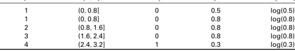
We illustrate the data transformation here for the simple case of survival data without covariates. Consider, for instance, the survival times of the two subjects in Table 1. The same data in the format of piece-wise exponential data (PED) is shown in Table 2. Each subject has as many entries (rows) as the number of intervals for which the subject is included in the risk set. Note that these rows can then be treated as independent (given covariates) within the estimation scheme. The intervals (j−1, j],
Table 1 Example of (conventional) time-to-event data for two subjects,i∈ {1,2}. Subjecti=1 is censored
att1=0.5 and subjecti=2 experienced an event att2=2.7
i ti ıi
1 0.5 0
2 2.7 1
Table 2 Data in the piece-wise exponential format with one row per interval in which a subject was in the
risk set. Intervals are defined byJ+1 cut-points0=0<· · ·< J=4;ıijis the status of subjectiin interval
j,tijthe time subjectispent in intervalj; the offset is denoted byoij=log(tij)
i j (j−1, j] ıij tij oij=log(tij) 1 1 (0,0.8] 0 0.5 log(0.5)= −0.69 2 1 (0,0.8] 0 0.8 log(0.8)= −0.22 2 2 (0.8,1.6] 0 0.8 log(0.8)= −0.22 2 3 (1.6,2.4] 0 0.8 log(0.8)= −0.22 2 4 (2.4,3.2] 1 0.3 log(0.3)= −1.20
j=1, . . . , J are specified by the user. Here, we chose equidistant intervals of length 0.8 as in Figure 1. Readers familiar with survival analysis will recognize this data structure to be very similar to the ‘start-stop’ format used to fit time-varying effects or effects of time-dependent covariates (TDCs) in the extended Cox regression model (Thomas and Reyes, 2014), with j−1 and j as start and stop times, respectively.
Further details and illustrations on transforming conventional time-to-event data into the format suitable to fit PEMs are provided in the data-transformation vignette (cf. Section 4 for details).
Note that another major advantage of this data structure is that (piece-wise constant) TDCs, that is, covariates that change their value over the follow-up period, can be incorporated naturally. In this case, the interval cut-pointsjmust additionally
include all time points at which changes in the TDC are recorded and model (2.2) is extended to the form i(t|xij)= jexp(xijTˇ) (cf. Section 3.4). Furthermore,
time-varying effects, where the association between a covariate and the hazard rate is allowed to change over the follow-up, can be incorporated by including an interaction term of the covariate with time t in the linear predictor (for more details, see Sections 3.3.2 and 3.3.3). This requires defining a TDC for time itself, for example, by settingtj :=j in the respective rows of the transformed data set.
Similarly, estimation of left-truncated data can be easily accommodated by excluding intervals before the respective left-truncation times as described by Guo (1993).
2.3 Piece-wise exponential Additive Mixed Model
Model (2.3) can be extended to include nonlinear or smoothly time-varying effects of time-constant or TDCs by incorporating semiparametric effects, that is, moving from a Poisson GLM representation to a Poisson GAMM representation. In reference to
the acronyms for PEMs and GAMs, we denote this model type by PAMM (piece-wise exponential additive mixed model). For a general PAMM, the hazard rate at time t for individualiwith covariate vectorxi is given by
i(t|xi)= exp f0(tj)+ p k=1 fk(xi,k, tj)+bi , ∀t∈(j−1, j], (2.4)
wheref0(tj) represents the log-baseline hazard rate (cf. Section 2.3.1) andfk(xi,k, tj),
k=1, . . . , p, denotes very general effect types, possibly of different complexity and potentially depending on both a covariate and time. In particular, smooth nonlinear and smoothly time-varying effects (cf. Section 2.3.2) of the time-constant confounders
x•k=(x1,k, . . . , xn,k)Tare included. The time variabletjis constant over each interval
to ensure that the estimated hazard rates still correspond to a PEM. Typical choices are interval end-points tj =j∀t∈(j−1, j], or interval mid-points tj =
j+j−1
2 ∀t∈ (j−1, j]. Additionally, bi denote random intercept terms (Gaussian frailty), where i, =1, . . . , Lis the cluster to which subjectibelongs. We do not discuss these terms
in this tutorial, but an example application is provided in the pammtoolsvignette frailty (cf. Table 7).
A common way to specify unknown smooth functions likef(x, tj) is to use splines,
which are represented by a weighted sum ofMbasis functions. A univariate function, such as the baseline hazardf0(tj), can be expanded asf0(tj)=Mm=10mBm(tj),with spline coefficients0mandbasis functionsBm(tj) (for a detailed description of splines,
see, for example, Ruppert et al., 2003). Increasing the number of basis functions for such terms increases their flexibility and also the danger of overfitting, while an excessively low number of basis functions might not provide the necessary flexibility. In PAMMs, this trade-off is resolved by specifying a relatively large number of basis functions and then penalizing ‘wiggliness’ of the estimate (e.g., by penalizing the difference between neighbouring basis coefficients in P-splines; Eilers and Marx, 1996). Technically, the penalization strength is controlled by separate smoothing parameters for each additive term, which are estimated simultaneously with all other model coefficients, for example, using restricted maximum likelihood (REML) estimation (Wood, 2011). This has the advantage that no strong assumptions about the shapes of such smooth effects are necessary in order to specify the model. Instead, they are estimated based on the data.
This idea can be extended to bivariate interaction surfaces, such as thefk(xi,k, tj)
terms in Equation (2.4), through the use of tensor product bases of the form f(xi,k, tj)=Mm=1L=1mBm(xi,k)B(tj). By specifying an interaction of covariates x•k with the (discretized) time tj, we can model (piece-wise constant) time-varying
effects of different grades of complexity, the most common of which are summarized in Table 3. Section 3.3 provides examples for most of these effects illustrated on widely known data sets. Note here that the effect types in Table 3 are merely a small subset of
Table 3 Overview of potentially smooth nonlinear and/or smoothly time-varying effect specifications in the analysis of time-to-event data
Effect Specification Description
ˇkxi,k+ˇk:tj·xi,k·tj: Linear, linearly time-varying effect
fk(xi,k) : Smooth nonlinear, time-constant effect
fk(xi,k)·tj: Smooth, linearly time-varying effect
xi,k·fk(tj) : Linear, smoothly time-varying effect
fk(xi,k, tj) : Smooth, smoothly time-varying effect
potential effect types. Further extensions such as spatial effects can be incorporated into Equation (2.4) just as easily, but they are beyond the scope of this tutorial.
Next (cf. Section 2.3.1), we illustrate the estimation of the baseline hazard with PEMs and PAMMs, and compare the results with the respective Nelson–Aalen estimates.
2.3.1 Baseline hazard
In the original definition of PEMs in (2.3), the baseline hazard is modelled by a step function with interval-specific hazardsj, which are estimated by including dummy
variables for each interval in the design matrix. This has two major drawbacks: 1. the choice of the interval cut-points as well as the number of intervals is rather
arbitrary (c.f. Demarqui et al., 2008); and
2. if a large number of cut-points is used, (too) many parameters need to be estimated and the individual estimates ˆjcan become unstable. If the estimation
of time-varying effects is required as well, this problem is exacerbated further. In PAMMs, the baseline hazard is modelled as a regression spline over time, using a suitably discretized time variabletj as earlier defined. Choosing a sufficiently large
number of intervals and spline basis functions, the baseline hazard can then be estimated very flexibly. At the same time, over-fitting is avoided via penalization and, hence, smooth and stable estimates are obtained.
In many real life applications, the (baseline) hazard changes quickly at the beginning of the follow-up and less so towards the end. In these cases, a fixed penalty for the whole spline may be too restrictive; thus an estimation of the baseline hazard using adaptive spline smooths, where the penalty applied to the basis coefficients can itself change over the course of the follow-up (i.e., smaller penalty at the beginning, stronger penalty towards the end) may be preferable (Wood, 2011). This, however, also implies a higher computational burden.
2.3.2 Smooth nonlinear, smoothly time-varying effects
The major advantage of PAMMs over currently available implementations of Cox-type or Aalen-type models is that the entire flexibility and methodological progress of GAMMs can be employed with regard to covariate effects, not only to
the reliable and smooth estimation of baseline hazard rates. The summandsfk(xi,k, tj)
in the second term in Equation (2.4) can represent a variety of different effect types, ranging from simple linear, time-constant effects xi,kˇk to nonlinear, time-constant
effects fk(xi,k) and nonlinear and smoothly time-varying effects fk(xi,k, tj). Table 3
summarizes the most common and important of these effect types. Time-varying effects are modelled as interaction terms between the covariate of interest, that is,
x•k, and the discretized timetj, that is, the corresponding interval end or mid-points.
All of these effect types can be specified fairly easily by the practitioner, for example, within the syntax of the gam function from the R-package mgcv (Wood, 2017), if the data is given in the format of Table 2 complemented by covariate information.
3 Applications and illustrations
In the following section, we describe and illustrate the application of PAMMs to various settings in time-to-event analysis and compare the estimates obtained from PAMMs with other established approaches on real data examples. For illustration, we use a follow-up restricted (t≤400) subset of the Veterans’ Administration lung cancer study (Kalbfleisch and Prentice, 1980), which is available in the survival (Therneau, 2015) package and is a widely used data example in the context of time-to-event analysis. In this study, males with advanced inoperable lung cancer were randomized to one of two treatment regimens for lung cancer, either standard or novel chemotherapy, represented by the binary variabletrt. In addition, the data set contains several time-constant covariates, namelycelltype(categorical) of the tumour, theage
(in years) at the beginning of treatment, the Karnofsky performance score (karno; 100=good) and a dummy variableprior, indicating whether there had been a prior therapy (0=no, 1=yes) along with survivaltimeand censoringstatus(0=censored, 1=event). Within the scope of this study, it is of major interest how the two different treatments in combination with the other covariates affect the survival of lung cancer patients. An excerpt of the data can be found in Table 4.
We omit the respectiveR-code here for clarity and brevity, however, each section refers to a dedicated vignette in thepammtoolspackage that contains code showing the practical work flow in full detail (cf. Section 4).
3.1 Estimating the baseline hazard
First, we demonstrate how to fit and visualize simple baseline models using the pammtools package. We use both a PEM and a PAMM and compare the results of the estimated baseline hazard to the conventional Nelson–Aalen estimator, which can be obtained, for example, by applying thecoxphfunction from thesurvival package directly on the veteran data from Table 4. In order to fit PEMs and PAMMs, however, we need to transform the data into the PED format, similar to the exemplary data presented in Table 2 using the split data function from the pammtoolspackage.
Table 4 Raw structure of the Veterans’ Administration lung cancer study data
trt celltype time status karno age prior
1 large 19 1 30 39 1 1 squamous 231 0 50 52 1 0 large 156 1 70 66 0 0 smallcell 51 1 60 67 0 1 smallcell 95 1 70 61 0 1 large 133 1 75 65 0
Table 5 Veterans’ Administration lung cancer study data after transformation to the piece-wise exponential data (PED) format (first six rows of subject 1)
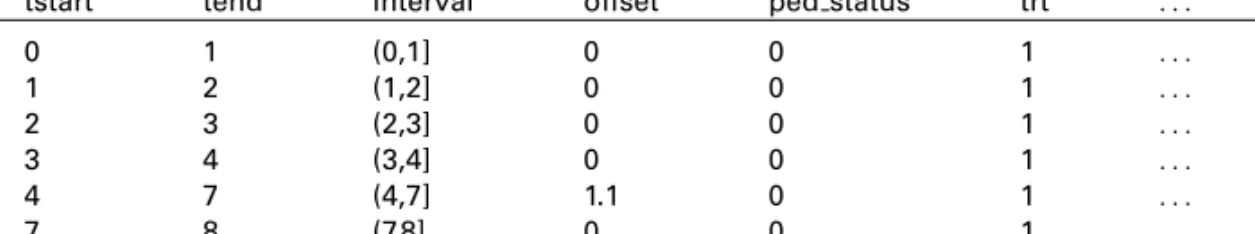
id tstart tend interval offset ped status trt . . . prior
1 0 1 (0,1] 0 0 1 . . . 1 1 1 2 (1,2] 0 0 1 . . . 1 1 2 3 (2,3] 0 0 1 . . . 1 1 3 4 (3,4] 0 0 1 . . . 1 1 4 7 (4,7] 1.1 0 1 . . . 1 1 7 8 (7,8] 0 0 1 . . . 1
Note that this data augmentation substantially increases the data set size: in this case, the original data from Table 4 contain n=131 individuals (=rows), while the data in piece-wise exponential format have 5 392 rows, if all unique event and censoring times are used as interval cut-points. In addition, several auxiliary variables are constructed, see Table 5. Based on the data from Table 5 and using the glm function, a simple baseline PEM can be fitted. The piece-wise constant hazards for each interval are obtained simply by treating the intervals themselves as a factor variable, which results in the model specification below (using standard dummy coding, with (0, 1] as the reference category): (t)=0(t)=
exp
ˇ0+Jj=2ˇ0jI(t∈(j−1, j])
, where I(t∈(a, b]) is the indicator function for t (taking value 1, if its argument is true, and 0 otherwise). Here, ˇ0 represents the
log baseline hazard in interval j= 1 and ˇ0j the log-hazard deviation in interval j
compared to intervalj= 1. When the partition of the follow-up period uses all event and censoring times as interval cut-points (and no ties are present), the regression effects of the Cox model and the PEM are equivalent (see also Section 2.1).
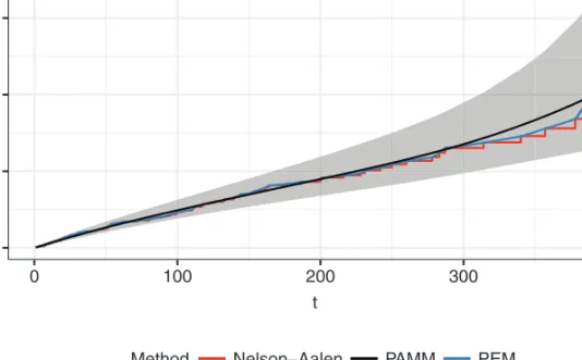
Alternatively, the baseline hazard can be modelled as a regression spline using ‘discretized time’tjas the covariate. A comparison of the different cumulative baseline
hazard functions is presented in Figure 2. While the cumulative hazards of the Cox PH model and the PEM are equivalent (at the interval end-points), the cumulative hazard obtained by fitting a PAMM is, not surprisingly, slightly different. Here, as in the following, the point-wise confidence intervals always refer to the PAMM estimates.
0 2 4 6 0 100 200 300 400 t Λ ^ (t )
Method Nelson−Aalen PAMM PEM
Figure 2 Comparison of the cumulative hazard estimates obtained by a Cox PH model (Nelson–Aalen), a PEM and a PAMM
3.2 Models including covariates
In this section, we incorporate conventional covariate effects into the models. We restrict ourselves to the case of time-constant covariates in this section, while the usage of TDCs is described in Section 3.4. We begin by fitting a classical Cox PH model to the original data from Table 4 using the coxph function, with a linear time-constant effect for the treatment variable (trt) and a nonlinear time-constant effect forkarno. The corresponding hazard is then specified by(t|x)= 0(t) exp
ˇ1I(trt= 1)+f(karno) ,where theageeffect is estimated using P-splines
(Eilers and Marx, 1996) and the ‘optimal’ degrees of freedom have been determined by Akaike’s Information Criterion (AIC) (Hurvich et al., 1998), which can be done by setting thedfargument of thecoxphfunction equal to zero.
Similarly, based on data in PED format (cf. Table 5), we can fit the corresponding PAMM, simply by including a nonlinear effect f(karno) into the linear predictor: (t|x)= exp(0(tj)+ˇ1I(trt= 1)+f(karno)).Actual estimation can be done by, for
example, using thegamfunction frommgcv. By default, thin plate regression splines are used for such effects in mgcv, but here we use P-splines for direct comparison with the Cox routine. The ‘optimal’ effective degrees of freedom (edf) can be chosen by maximizing a generalized cross validation, REML or ML criterion (Wood, 2011, 2017).
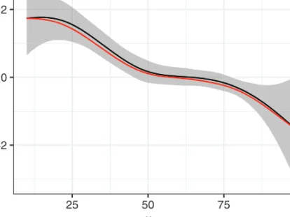
Figure 3 displays the comparison of the smooth effect estimates obtained by the two approaches. Both effects exhibit a decreasing effect with increasing Karnofsky score (KS;edf: 4.03 for Cox; 4.02 for PAMM) and have very similar shapes. The effect
−2 0 2 25 50 75 100 x karno f ^ (x k a rno) Method Cox PH PAMM
Figure 3 Comparison of nonlinear Cox PH model and PAMM estimates
of treatment is not significantly different from zero for both approaches (p-values of corresponding t-tests: 0.11 for Cox; 0.16 for PAMM).
3.3 Time-varying effects
In the following sections, we focus on time-varying effects, that is, effects of the form f(x, t) for varying degrees of complexity as summarized in Table 3, and illustrate the specification of these different effect types as well as their estimation with PAMMs. 3.3.1 Stratified baseline
In many cases, it is unreasonable to assume that the baseline hazard is the same for subjects on different levels of a categorical variable. In that case, the PH assumption is violated. To avoid this issue, the so-calledstratifiedPH models (Klein and Moeschberger, 1997, Ch. 9.3; also stratified Cox model in the context of Cox models) have been proposed, where a separate baseline is estimated for each sub group, while the effects of other covariates are identical for all subjects. Letz be a categorical variable with categoriesk= 1, . . . , K. A PH model stratified with respect tozis then defined by
(t|z, x)=0k(t) exp(xˇ), (3.1)
where 0k(t) are the group-specific baseline hazards. In the Cox framework, ˇ is
estimated through the partial likelihood approach as usual and the baseline0k(t) is
squamous smallcell adeno large 0 100 200 300 400 0 100 200 300 400 0 100 200 300 400 0 100 200 300 400 0 3 6 9 t Λ ^ (t )
Method stratified Cox stratified PAMM
Figure 4 Cumulative hazard estimates using a stratified Cox compared to a stratified PAMM approach
In the context of PAMMs, the group-specific baseline hazards can be regarded as an interaction of the formf(tj)·zbetween a (nonlinear) function of (discretized) time
and a categorical variable, as defined in Equation (3.2):
(t|z,x)=expf0k(tj)I(z=k)+xˇ . (3.2)
Here, the individual baseline hazards are again represented via linear combinations of known basis functions B(·) and estimated basis coefficients , such that f0k(tj) =Mm=10kmBm(tj). In the aforementioned notation, we absorbed group-specific
intercepts ˇ0k (i.e., main effects of z) into the baseline terms f0k for brevity. When
specifying the model inR, however, the group variablezmust usually be included as a separate effect as well (cf. the strata vignette in Table 7).
For illustration consider patients with different cell types in the Veteran’s data. Figure 4 shows the cumulative baseline hazard estimates for the different cell types using stratified Cox and stratified PAMM procedures, indicating that the two models are in good agreement. One difference between the two models, as fitted in the example, is the choice of cut-points. For the stratified Cox model, cut-points occur at respective event times in the different groups, while in the stratified PAMM model, identical cut-points are used to estimate the baseline hazards in all groups.
3.3.2 Linear, nonlinearly time-varying effects
Next, we showcase effects of the form f(t)·x, where x is continuous. In the GAMM literature, these models are known as varying coefficient models (Hastie and Tibshirani, 1993); here the effect of x varies over time and thus constitutes a
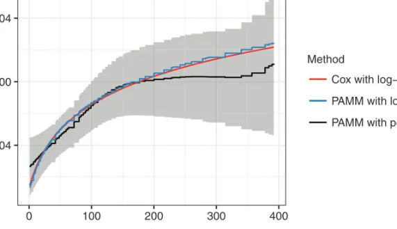
−0.04 0.00 0.04 0 100 200 300 400 t f ^ (t ) Method
Cox with log−transform PAMM with log−transform PAMM with penalized spline
Figure 5 Comparison of estimates for the nonlinearly time-varying effect of the Karnofsky score
classical use case of time-varying effects. Note that the inclusion of time-varying effects invalidates the PH assumption, thus this additional flexibility can complicate interpretation. For illustration, we fit a time-varying effect of the KS (xkarno). For this
association, a specific logarithmic functional form of the time variationf(xkarno, t)=
f(t)·xkarno=
ˇkarno+ˇkarno,tlog(t+20) ·xkarno is frequently assumed. (Compare
discussion in thetimedepvignette of thesurvival package.)
In the PAMM context, such effects can be specified by a linear interaction between
xkarnoand a log(tj+20) transformation of (discretized) time. However, usually we do
not know the precise functional form off(tj) in advance and want to estimate it from
the data, such that(t|x)=exp(f0(tj)+f(tj)·xkarno). This can be done, for example,
by representingf(tj)·xkarno=
M m=1
mBm(tj) ·xkarnoin a basis function expansion
as described in Section 2.3. Figure 5 shows that, in this case, the differences between the estimates using a pre-specified transformation of time and estimates off(tj) using
semiparametric regression are negligible, although the semiparametric estimate seems to ‘level off’ aftert=150.
3.3.3 Nonlinear, nonlinearly time-varying effects
In this section, we consider effects of the form f(x, t), where we assume that x potentially has a nonlinear effect that also varies over time nonlinearly, estimated by penalized splines. We continue the example from Section 3.3.2, except that now
f(xkarno, tj) will be modelled as a two-dimensional smooth function using a tensor
product representation, such thatf(xkarno, tj)=
M m=1
L
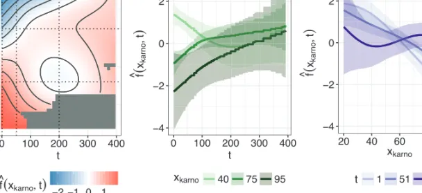
0 100 200 300 400 25 50 75 100 t xkarno −2 −1 0 1 f ^( xkarno, t) −4 −2 0 2 0 100 200 300 400 t f ^ (x karno , t) xkarno 40 75 95 −4 −2 0 2 20 40 60 80 100 xkarno f ^ (x karn o , t) t 1 51 200
Figure 6 A heat map visualization of the nonlinear, nonlinearly time-varying effect of the KS variable on the log-hazard scale (left panel). The middle and right panel of the figure depict slices through the left panel, fixing either specific values of the KS (mid panel) or specific values of time (right panel). Grey
regions in the left panel reflect combinations ofxkarnoandtwhere no data was observed. Intervals are
point-wise±2 standard deviations. Note that the heat map represents a step function over time; we show a
smooth surface instead for better presentation
The resulting estimate is depicted in Figure 6. Focusing onvertical‘slices’ through the heat map on the left, we can see the effect of the KS at different times. For example, at the beginning of the follow-up (t=1), low KS values are associated with higher hazards, while high KS values are associated with lower hazards, that is, very similar to the smooth, time-constant effect in Figure 5. For later time points (e.g., t=200), the effect of KS is more homogeneous and generally closer to zero, even for extreme values of KS. Focusing onhorizontal‘slices’ through the heat map on the left, on the other hand, we can see how the hazard associated with different KSs changes over time. A KS of 40, for example, is associated with a much higher hazard (and, hence, decreased survival probability) at the beginning, decreases after some time and then increases again slightly, while patients with a KS close to 100 seem to have a lower hazard at the beginning, which increases towards the end of the follow-up.
This is consistent with a frequent observation in medical studies showing that the association between health scores measured at baseline and hazard rates becomes weaker or even diminishes completely over the course of the follow-up. Such a conclusion can be drawn here as well, considering the high uncertainty of the estimates for later time points. Thus, such bivariate effect functions can provide a more complete and realistic picture of time variation in the association between the hazard and the KS at baseline (increasing towards 0 for higher KS values, decreasing towards 0 for lower KS values), compared to the analyses presented in Sections 3.2 and 3.3.2.
3.4 Time-dependent covariates
Here, we describe how one can incorporate TDCs in the framework of PAMMs. Because the Veteran’s data does not contain TDCs, we switch to a different standard example known from the literature, the well-known recidivism data first presented in Rossi et al. (1980). The data contains information on 432 convicts released from prison. The outcome of the study was the number of weeks until the first rearrest. Maximal follow-up time was 52 weeks. Baseline covariates include financial aid (fin; yes/no),ageat time of release (in years),race(black/other), work experience prior to incarceration (wexp; yes/no), marital status (mar; married/unmarried), released on parol (paro; yes/no) and number of prior convictions (prio).
Furthermore, the data set contains a TDC, which indicates the weekly employment status for each subject until end of follow-up or first rearrest. For comparison, we largely follow the extensive analysis of the data presented in Fox and Weisberg (2011), who use extended Cox regression, except that we model the effects of age and prior convictions using P-splines (Eilers, 1998). In this example, the data transformation required to fit the Cox model is equivalent to the data transformation needed to apply PAMMs. More precisely, we create a data set where each subject has one row for each week of follow-up, as the employment status can potentially change every week.
A subset of the transformed data is presented in Table 6, exemplary for subjects 1 and 2. Note that the event indicator (arrest) is 0 up to the week of the event. Covariates other than employment remain constant over time. Note that the employment variable is ‘lagged’ by one week as it is unknown if unemployment preceded arrest or vice versa in any given week. Consequently, the data start with the interval (1,2], as the ‘lagged’ employment status for week 1 (interval (0,1]) would not be defined. Note that we can exclude the offsetoijfor these weekly data, as it is log(1)= 0 for all observations.
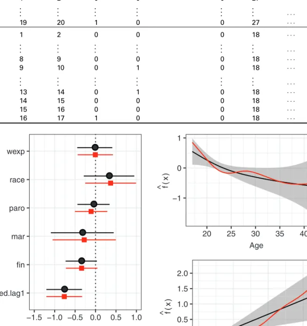
Figure 7 displays the comparison of the extended Cox regression and PAMM applied to the recidivism data. Both the fixed coefficients (left panel) and the smooth estimates (right panel) are generally in good agreement.
However, the nonlinear estimates of the Cox model are more ‘wiggly’ compared to the PAMM estimates (using default settings for both algorithms), which reflects the different approaches for the selection of the optimal smoothness penalty parameters. Being employed in the previous week is clearly associated with a decreased hazard of rearrest compared to being unemployed in the previous week. So convicts that recently had a job seem to be less likely to be arrested. For both the PAMM and the Cox PH approach the remaining fixed effects are not significant. Finally, it turns out that for both modelling approaches, increased age is generally associated with a decreased hazard, whereas convicts with a high number of prior convictions are more likely be rearrested. However, while for the Cox PH approach both effects are rather wiggly, the PAMM estimates are almost linear and very smooth and, hence, somewhat easier to interpret.
Note that we only consider the employment status of the previous week, thus the marginal hazard increase in week 21 for a subject that was employed for 19 weeks and is unemployed in week 20 is the same as for a subject that was unemployed from
Table 6 Exemplary data in counting-process format needed to fit extended Cox regression and PAMMs. Subject 1 was unemployed throughout the follow-up and rearrested in week 20, subject 2 was unemployed until week 8, found employment for weeks 9 through 13 and became unemployed again thereafter (data in the table with lag = 1). In week 17, the subject was rearrested. The other covariates are only measured at baseline and remain constant
subject start stop arrest employed (lag = 1) fin age · · · mar
1 1 2 0 0 0 27 · · · 0 . . . . . . . . . . . . . . . . . . . . . · · · . . . 1 19 20 1 0 0 27 · · · 0 2 1 2 0 0 0 18 · · · 0 . . . . . . . . . . . . . . . . . . . . . · · · . . . 2 8 9 0 0 0 18 · · · 0 2 9 10 0 1 0 18 · · · 0 . . . . . . . . . . . . . . . . . . . . . · · · . . . 2 13 14 0 1 0 18 · · · 0 2 14 15 0 0 0 18 · · · 0 2 15 16 0 0 0 18 · · · 0 2 16 17 1 0 0 18 · · · 0 ● ● ● ● ● ● ● employed.lag1 fin mar paro race wexp −1.5 −1.0 −0.5 0.0 0.5 1.0 β^± 1.96 ⋅SE
Method ●● PAMM Cox−PH
−1 0 1 20 25 30 35 40 45 Age f ^ (x ) −0.5 0.0 0.5 1.0 1.5 2.0 0 5 10 15
Number of prior convictions
f
^ (x
)
Figure 7 Left panel: Coefficient estimates using extended Cox regression and PAMM, respectively. Points indicate the estimates on the log-hazard scale. Error bars indicate the 95% confidence intervals. Right panel: Smooth estimates for age (top) and number of prior convictions (bottom)
Table 7 Overview of vignettes and their content provided in the packagepammtools. To access the vignettes visit https://adibender.github.io/pammtools/articles/
Vignette Description
Data transformation Details (and respectiveR-code) on transformation of conventional time-to-event data
into PED format (cf. Section 2.2)
Basics Basic modelling and equivalence to Cox PH model
Baseline Baseline estimation and visualization (cf. Section 2.3.1)
Splines Linear, time-constant effects of the formfk(xi,k) (cf. Section 3.2)
Strata Stratified PH modelsfk(t)I(z=k) (cf. Section 3.3.1)
TV effects Details on fitting models with time-varying effects of different complexity, for example,
xi,k·fk(t) orfk(xi,k, t) (cf. Section 3.3.2 and 3.3.3)
TD covariates Details on fitting models with time-varying covariates (cf. Section 3.4)
Frailty Example of fitting Gaussian frailty models and comparison to thecoxmepackage.
Convenience Demonstration of convenience functions for pre-/post-processing of PEMs/PAMMs,
visualization and model comparisons
the beginning. A more complex analysis would account for the complete employment history, that is, use a cumulative effect of employment, for example via the weighted cumulative exposure (WCE) approach (Sylvestre and Abrahamowicz, 2009), such thatf(x, t)=u≤t =w(t−u)x(u), where weights w(t−u) can again be estimated using penalized splines or similar approaches. An implementation of this method can be found in the correspondingR-packageWCE. Bender et al. (2016) describe an implementation of such effects for PAMMs.
4 Software
While PAMMs are essentially GAMMs, and any statistical software (or programming language) could be used to fit these models, the technicalities of data transformation, interpretation and visualization often hinder their application by practitioners in our experience. Therefore, in addition to this tutorial, we also provide an R add-on package called pammtools (Bender and Scheipl, 2017); for the most current version of the package visit https://adibender.github.io/ pammtools/ which provides convenience functions that facilitate the application of PAMMs. Individual sections and concepts described in this article are accompanied by vignettes on the pammtools homepage that illustrate the concrete application in the statistical programming language R (R Core Team, 2016). Table 7 gives an overview of all vignettes currently available on the site. Most conveniently, the vignettes can be accessed directly from the homepage at https://adibender.github.io/pammtools/articles. Additionally, you can call?pammtoolsto obtain a package overview and links to the individual vignettes. The package (and its vignettes) thus also serves as the code supplement for this article (see also Bender et. al 2018).
Although this article is focused on R and on fitting the PEMs/PAMMs with the mgcvpackage, any software that can fit GL(M)Ms or GA(M)Ms could be used to fit
this model class. For example, the standardglmfunction could be used to fit PEMs, but does not offer many of the advanced functions frommgcv::gamand offers no penalized estimation of smooth effects. Additionally, the package pch provides the functionpchreg, that fits a variation of PEMs for right-censored and left-truncated data using a custom routine, but does not offer penalized estimation or other convenience functions for pre- and post-processing (Frumento, 2016). If random effects (or frailty terms, as they are usually referred to in survival analysis) need to be included, the lme4 library (Bates et al., 2015) offers many options, although simple random effect structures are also supported bymgcv::gam. Note that Cox PH models are also supported bymgcv(family="cox.ph"), thus penalized estimation of smooth, nonlinear effects of time-constant covariates fk(xk) are also directly
available for the Cox model. However, these cannot be used to fit the extended Cox model with time-varying effects or TDCs. Memory efficient big data estimation with the functionbamis also not available forfamily="cox.ph".
In addition, regularization techniques such as the LASSO and model-based boosting, for example, via glmnet (Friedman et al., 2010) or mboost (Hothorn et al., 2016), respectively, can also be applied to PEMs and PAMMs. Although the glmnetpackage has recently implemented Cox models (see Simon et al., 2011), only rather simple Cox models can be fitted. For example, neither TDCs nor nonlinear effects are available. Ifglmnetis used to fit a PEM, however, TDCs can be included. Within the framework of mboost, the glmboost routine with argument family = CoxPH() can be used for time-to-event data, if the PH assumption holds but does not allow for TDCs. With model-based boosting of PAMMs via mboost’s gamboost() function for fitting GAMs (compare, e.g., Hothorn and B ¨uhlmann, 2006), the entire flexibility of boosted GAMMs is available for survival analysis, however. For more general details on boosting methods, compare also the tutorial on boosting approaches by Mayr and Hofner (2018) in this special issue.
5 Discussion
The focus of this tutorial article has been on the application of semiparametric regression in the context of continuous time survival analysis using piece-wise exponential (additive mixed) models, which we denote by PEMs and PAMMs. We first introduced the general idea of the classical PEM and then described its semiparametric extension, the PAMM. We illustrated the use of both approaches, starting with the required pre-processing and data augmentation steps and simple standard models, and then turned to successively more advanced applications. In this way, we hope to provide practitioners with a useful addition to their methodological toolbox for time-to-event data analysis, which is firmly embedded in the familiar context of GAMMs, allowing them to exploit the robust, well-documented and highly developed software implementations available for this model class.
The results of PEMs and PAMMs are generally in good agreement with conventional Cox-type modelling for most applications, and the concrete choice of model type can depend on many factors, including familiarity, availability of software implementations, data structure and so on. In the following, we summarize some of the strengths of PAMMs that may guide the decision process:
• Firmly grounded in modern penalization methods, PAMMs are a legitimate method for the analysis of time-to-event data and not just a ‘hack’ that can be used in case other options fail. For example, in Section 3, we demonstrated that we can use PEMs/PAMMs to obtain estimates very similar to the estimates of Cox-type models. While it is true that for simple use cases where the PH assumption holds the Cox model has a clear advantage over PAMMs in terms of computational cost since the data does not have to be expanded, these advantages disappear whenever time-varying effects or TDCs need to be included (cf. Sections 3.3 and 3.4). In our experience, the differences in computation time for standard applications are usually negligible anyway.
• While Cox models may have computational advantages in simpler use cases (e.g., when the PH assumption holds and the data do not have to be expanded), their computational advantage diminishes whenever time-varying effects or TDCs need to be included (cf. Sections 3.3 and 3.4). In fact, PAMMs could be more efficient in some cases, as the extended Cox model requires splits at each event time, while split points for PAMMs could be chosen more crudely.
• In the past, methodological and algorithmic advances in semiparametric regression first became available in the framework of GAMMs. Thus, for example, the important innovations implemented in the mgcv package, such as REML-optimal estimation of penalized effects (Wood et al., 2016), reliable and generally applicable tests for semiparametric terms (Wood, 2012), locally adaptive spline smooths (Wood, 2011), double-penalty variable selection strategies that can shrink effect estimates to zero (Marra and Wood, 2011) similar to the (group) LASSO (Meier et al., 2008), highly memory efficient estimation on huge data sets (Wood et al., 2016), and many more, are directly available for the estimation of PAMMs. Similarly, in the past, regularization approaches such as boosting became available for GAMMs long before being ported to Cox-type models.
• In Section 3.3.2, it was shown how easily linear but nonlinearly time-varying effects of the form f(t)·x can be incorporated in the framework of PAMMs, being directly available within the syntax of gam. In contrast, in conventional Cox modelling either a particular functional form of the time variation has to be assumed (as illustrated in Section 3.3.2) or further pre-processing steps become necessary, such as manual construction of the corresponding spline design matrices in combination with suitable penalization (see, e.g., the simulation study in Groll et al., 2017, for an application of this strategy).
• TDCs can be embedded in this framework naturally (cf. Section 3.4), and even more complicated effects of TDCs, for example, the WCE approach by
Sylvestre and Abrahamowicz (2009) or the DLNM of Gasparrini et al. (2017), where cumulative time-varying effects of TDCs are considered, can be directly incorporated with fairly little additional effort.
With respect to assessment of model quality in the context of PEMs/PAMMs, we advise not to use conventional measures like, for example, the deviance, but rather use dedicated measures developed specifically for survival analysis such as the Brier score or the concordance index (Gerds et al., 2013), which have the secondary advantage of being directly comparable with evaluation metrics for other model classes for survival analysis. Finally, note that in this article we did not address any issue regarding estimation or inference, for which we refer to Wood (2017, 2011).
References
Andersen PK, Borgan O, Gill R and Keiding N (1992) Statistical Models Based on
Counting Processes. Berlin and New York,
NY: Springer-Verlag.
Argyropoulos C and Unruh ML (2015) Analysis of time to event outcomes in randomized controlled trials by generalized additive models.PLoS ONE,10, e0123784. doi:10. 1371/journal.pone.0123784
Bates D, M ¨achler M, Bolker B and Walker S (2015) Fitting linear mixed-effects models using lme4. Journal of Statistical Software,
67, 1–48. doi:10.18637/jss.v067.i01 Bender A and Scheipl F (2017, November 14).
adibender/pammtools: v0.0.3.2 (Version
v0.0.3.2). Zenodo. URL http://doi.org/ 10.5281/zenodo.1048832
Bender A, Groll A and Scheipl F (2018, January
14). adibender/pammtutorial-smj: Release
v1.0.1 (Version v1.0.1). Zenodo. URL
http://doi.org/10.5281/zenodo.1147058 Bender A, Scheipl F, K ¨uchenhoff H, Day AG and
Hartl W (2016) Modeling exposure-lag-response associations with penalized
piece-wise exponential models(Technical report
108). Ludwig-Maximilians-University URL https://epub.ub.uni-muenchen.de/ 32010/.
Berger M and Schmid M (2018) Semiparametric regression for discrete time-to-event data.
Statistical Modelling,18, 322–45.
Clayton DG (1983) Fitting a general family of failure-time distributions using GLIM.
Journal of the Royal Statistical Society.
Series C (Applied Statistics),32, 102–109.
doi:10.2307/2347288
Cox DR (1972) Regression models and life tables (with discussion). Journal of the Royal
Statistical Society,B 34, 187–220.
Demarqui FN, Loschi RH and Colosimo EA (2008) Estimating the grid of time-points for the piecewise exponential model. Lifetime
Data Analysis, 14, 333–56. doi:10.1007/
s10985-008-9086-0
Eilers PHC (1998) Hazard smoothing with B-splines.Proceedings of the 13th
Interna-tional Workshop on Statistical Modelling,
New Orleans, La, pages 200–07..
Eilers PHC and Marx BD (1996) Flexible smoo-thing with B-splines and penalties.
Statis-tical Science, 11, 89–121. doi:10.1214/ss/
1038425655
Fox J and Weisberg HS (2011)An R Companion
to Applied Regression. Thousand Oaks, CA:
SAGE. ISBN 978-1-4129-7514-8.
Friedman M (1982) Piecewise exponential models for survival data with covariates. The
Annals of Statistics,10, 101–13.
Friedman J, Hastie T and Tibshirani R (2010) Regularization paths for generalized linear models via coordinate descent. Journal of
Statistical Software,33, 1–22.
Frumento P (2016) pch: Piecewise constant hazards models for censored and truncated data. R package version 1.3. URL https:// CRAN.R-project.org/package=pch
Gasparrini A, Scheipl F, Armstrong B and Kenward MG (2017) A penalized frame-work for distributed lag non-linear models.
Biometrics. doi:10.1111/biom.12645
Gerds TA, Kattan MW, Schumacher M and Yu C (2013) Estimating a time-dependent concordance index for survival prediction models with covariate dependent censoring.
Statistics in Medicine,32, 2173–84. doi:10.
1002/sim.5681
Groll A, Hastie T and Tutz G (2017) Selection of effects in Cox frailty models by regulari-zation methods.Biometrics,73, 846–56. Guo G (1993) Event-history analysis for
left-truncated data. Sociological Methodology,
23, 217–43. doi:10.2307/271011
Hastie T and Tibshirani R (1993) Varying-coeffi-cient models.Journal of the Royal Statistical
Society. Series B (Methodological), 55,
757–96. doi:10.2307/2345993
Holford TR (1980) The analysis of rates and of survivorship using log-linear models.
Biom-etrics,36, 299–305. doi:10.2307/2529982
Hothorn T and B ¨uhlmann P (2006) Model-based boosting in high dimensions.
Bioinfor-matics,22, 2828–29.
Hothorn T, B ¨uhlmann P, Kneib T, Schmid M and Hofner B (2016)mboost:Model-based boo-sting. R package version 2.7-0. URL http:// CRAN.R-project.org/package=mboost/ Hurvich CM, Simonoff JS and Tsai C (1998)
Smoothing parameter selection in non-parametric regression using an improved Akaike information criterion.Journal of the Royal Statistical Society: Series B (Statistical
Methodology),60, 271–93.
Kalbfleisch J and Prentice R (1980)The Statistical
Analysis of Failure Time Data. New York,
NY: Wiley.
Klein JP and Moeschberger ML (1997)Survival Analysis: Techniques for Censored and
Truncated Data.New York, NY: Springer.
Laird N and Olivier D (1981) Covariance analysis of censored survival data using log-linear analysis techniques. Journal of the
American Statistical Association,76, 231–
40. doi:10.2307/2287816
Marra G and Wood SN (2011) Practical variable selection for generalized additive
models. Computational Statistics & Data
Analysis,55, 2372–87. doi:10.1016/j.csda.
2011.02.004
Martinussen T and Scheike TH (2006) Dynamic
Regression Models for Survival Data. New
York, NY: Springer.
Mayr A and Hofner B (2018) Boosting for statistical modelling: A non-technical intro-duction. Statistical Modelling,18, 365–84. Meier L, Van de Geer S and B ¨uhlmann P (2008) The group LASSO for logistic regression.
Journal of the Royal Statistical Society, B
70, 53–71.
R Core Team (2016) R: A Language and
Env-ironment for Statistical Computing. Vienna:
R Foundation for Statistical Computing URL https://www.R-project.org/
Rodr´ıguez-Girondo M, Kneib T, Cadarso-Su ´arez C and Abu-Assi E (2013) Model building in nonproportional hazard regression.
Statistics in Medicine,32, 5301–14. doi:10.
1002/sim.5961
Rossi PH, Berk RA and Lenihan KJ (1980)Money, Work, and Crime: Experimental Evidence.
New York: Academic Press.
Ruppert D, Wand MP and Carroll RJ (2003)
Semiparametric Regression. Cambridge:
Cambridge University Press.
Sennhenn-Reulen H and Kneib T (2016) Struc-tured fusion LASSO penalized multi-state models.Statistics in Medicine. doi:10.1002/ sim.7017
Simon N, Friedman J, Hastie T and Tibshirani R (2011) Regularization paths for Cox’s pro-portional hazards model via coordinate descent. Journal of Statistical Software,
39, 1.
Sylvestre M-P and Abrahamowicz M (2009) Flexible modeling of the cumulative effects of time-dependent exposures on the hazard.
Statistics in Medicine, 28, 3437–53.
doi:10.1002/sim.3701
Therneau TM (2015) A package for survival
analysis in S. R package version 2.38. URL
http://cran.us.r-project.org/web/packages/ survival/index.html
Thomas L and Reyes EM (2014) Tutorial: Survival estimation for Cox regression models with time-varying coefficients using
SAS and R. Journal of Statistical Software,
Code Snippets, 61. URL http://www.
jstatsoft.org/v61/c01
Whitehead J (1980) Fitting Cox’s regression model to survival data using GLIM.Journal of the Royal Statistical Society. Series C
(Applied Statistics), 29, 268–75. doi:10.
2307/2346901
Wood SN (2011) Fast stable restricted maximum likelihood and marginal likelihood esti-mation of semiparametric generalized linear models. Journal of the Royal Statistical
Society: Series B (Statistical Methodology),
73, 3–36.
——— (2012) On p-values for smooth compo-nents of an extended generalized additive model. Biometrika,100, 221–28. doi:10. 1093/biomet/ass048
——— (2017)mgcv: Mixed GAM Computation Vehicle with GCV/AIC/REML Smoothness
Estimation. URL http://cran.r-project.org/
web/packages/mgcv/index.html
Wood SN, Li Z, Shaddick G and Augustin NH (2016) Generalized additive models for gigadata: Modelling the UK black smoke network daily data.Journal of the American
Statistical Association, 1–40. doi:10.1080/
01621459.2016.1195744
Wood SN, Pya N and Saefken B (2016) Smoothing parameter and model selection for general smooth models. Journal of the American
Statistical Association, 111, 1548–63.