Sample size and robust marginal methods for cluster-randomized trials with censored event times

Sample size and robust marginal methods for

cluster-randomized trials with censored event times

YUJIE ZHONG

Department of Statistics and Actuarial Science

,

RICHARD J COOK

Department of Statistics and Actuarial Science, University of Waterloo, Waterloo, ON, N2L 3G1, Canada

E-mail: [email protected]

Summary

In cluster-randomized trials, intervention effects are often formulated by specifying marginal models, fitting them under a working independence assumption, and using robust variance esti-mates to address the association in the responses within clusters. We develop sample size criteria within this framework, with analyses based on semiparametric Cox regression models fitted with event times subject to right censoring. At the design stage, copula models are specified to en-able derivation of the asymptotic variance of estimators from a marginal Cox regression model and to compute the number of clusters necessary to satisfy power requirements. Simulation stud-ies demonstrate the validity of the sample size formula in finite samples for a range of cluster sizes, censoring rates and degrees of within-cluster association among event times. The power and relative efficiency implications of copula misspecification is studied, as well as the effect of within-cluster dependence in the censoring times. Sample size criteria and other design issues are also addressed for the setting where the event status is only ascertained at periodic assessments and times are interval censored.

Keywords: censored data; cluster-randomized trials; copula models; robust inference; sample size This is the peer reviewed version of the following article: Zhong Yujie, and Cook Richard J. (2015), Sample size and robust marginal methods for cluster-randomized trials with cen-sored event times, Statist. Med., 34, pages 901-923. doi: 10.1002/sim.6395, which has been published in final form athttp://dx.doi.org/10.1002/sim.6395. This article may be used for non-commercial purposes in accordance With Wiley Terms and Conditions for Self-Archiving:http://olabout.wiley.com/WileyCDA/Section/id-820227.html#terms

1

I

Cluster randomization is employed in clinical trials when it is appropriate on ethical [1], practical [2], or contextual [3] grounds to assign groups of individuals (e.g. families, schools, hospitals, or com-munities) to receive one of two or more interventions. In studies aiming to reduce the spread of infectious disease, for example, prevention strategies are most naturally administered to large groups of individuals (e.g. municipalities), and the resulting evidence of impact thereby reflects direct effects

(susceptibility), indirect effects (infectiousness of others), and the effect of herd immunity [4]. Cluster randomization also offers a way of minimizing contamination across treatment groups and can often enhance compliance [5, 6]. In some fields of research, the units providing the response are paired or otherwise grouped, as is the case in ophthalmology or audiology. In such settings, interventions that are administered and act through the blood stream (e.g. medications) necessitate randomizing indi-viduals, and the units providing the response are clustered within individuals. The many advantages of cluster randomization have led to its increased use in recent years in diverse areas of research in-cluding health promotion [7], education for disease management [8], clinical research [9], and health policy and program evaluation [10]. Donner and Klar [11] give a thorough account of the practical and methodological issues in the conduct of cluster-randomized trials.

While much of the methodological work on cluster-randomized trials to date has been for con-tinuous or binary responses, in many settings interest lies in evaluating the effect of an intervention in delaying or preventing the occurrence of an event. In patients with insulin-dependent diabetes mellitus, for example, interest may lie in the effect of medical therapies on the time to severe vision loss in each eye [12]; such times are correlated within individuals due to shared exposure to blood sugar levels, blood pressures, and other systemic features. Chronic otitis media is a condition aris-ing in children characterized by poor drainage of fluid from the inner ear. A common intervention involves the surgical insertion of a ventilating tube and interest then may lie in assessing an experi-mental post-surgery medical therapy designed to prolong the function of the ventilating tubes. The child is then the unit of randomization [13, 14], and the times to failure of the tubes in the left and right ears would naturally be correlated. Settings involving time to event responses with larger cluster sizes include studies of fall prevention in retirement homes [15], studies of primary care practices and survival in patients with depression [16], and studies of pediatric clinics and time to discontinuation of breast-feeding [17].

Cox regression models involving random effects, or frailty terms, are widely used for analysing correlated time to event data [18, 19]. In this framework failure times are typically considered to be independent conditional on a latent variable representing unexplained differences between clus-ters, and the association among responses within clusters arises by marginalizing over the random effects. There are several important limitations of this approach for the analysis of event times in cluster-randomized trials. First, specification of a proportional hazard model given cluster-level ran-dom effects is unappealing when the treatment indicator is fixed at the cluster level [20, 21]. Second, regression coefficients reflect the multiplicative effects of the intervention, conditional on the latent variable; the proportional hazards assumption does not hold in the marginal model obtained by inte-grating out the random effects, making the interpretation of the intervention effect challenging. Third, while the dependence within clusters is accommodated in the marginal joint distribution, the associ-ation is not modeled in an appealing way. Simple measures of within-cluster dependence do not in general arise from the random effects formulation with censored failure time data, so it is difficult to extract useful information for the design of future similar trials.

Methods involving intervention effects specified on the basis of marginal Cox models feature none of these limitations and are therefore much more appealing. For large numbers of small groups of correlated failure time, Lee et al. [12] developed very useful methods for robust inference about regression coefficients in marginal Cox models fitted under a “working independence” assumption, similar in spirit to the working independence assumption adopted when clustered categorical data are analysed via generalized estimating equations [22] or when multivariate failure time data are analysed by the marginal approach of Wei et al. [23, 24]. Robust “sandwich” variance estimates provided by Lee et al. [12] ensure valid inference when there is within-cluster dependence in event times. The simple marginal interpretation of intervention effects and use of robust variance estimation make this a useful and simple framework for the analysis of event times in cluster-randomized trials.

formu-lae for the cluster-randomized trials with continuous and discrete outcomes [5, 25–28], but relatively little work has been done for trials involving censored event times; in what follows, the term sample size is used to mean the number of clusters. Jahn-Eimermacher et al. [29] developed sample size criteria on the basis of a frailty model for the within-cluster dependence, but as mentioned earlier the frailty approach is unappealing for use in cluster-randomized trials. Manatunga and Chen [14] derived sample size formula for bivariate event times under a parametric proportional hazards model with exponential margins. Jung [30] proposed a simulation-based sample size calculation procedure involving a weighted rank test for clustered survival data, which allows variable cluster size. Moer-beek [31] studied the effect of sample size on precision of parameter estimates and statistical power for clustered randomized trials with discrete event times based on a generalized linear mixed model. Xie and Waksman [32] adapted the usual sample size criteria for log-rank tests by the introduction of a design effect involving the average cluster size and the intraclass correlation coefficient of the censoring (i.e., status) indicator of the response times. While the formula is relatively simple, the sample size criterion is based on an approximation of the asymptotic distribution of regression coef-ficients. More importantly, because the intraclass correlation coefficient in their design effect is for the censoring indicators rather than the underlying failure times, its magnitude is driven by both the dependence in the failure times within clusters and the within-cluster dependence in the censoring times. As a result, the event times may be independent within clusters, for example, but the censoring indicators may be highly correlated within clusters if the censoring times are dependent. Moreover, the correlation in the censoring indicators depends on both the administrative censoring time and the distribution of the random censoring time, so any plans to modify a study by extending follow-up or attempting to reduce loss to follow-up will render the measure of within-cluster dependence invalid.

We derive sample size criteria for cluster-randomized trials with censored time to event responses when the intervention effect is specified through a marginal semiparametric proportional hazards model fitted under a working independence assumption, and robust variance estimates are used as in Lee et al. [12]. Of course at the design stage a fully parametric model is required so a Weibull proportional hazard model is adopted to accommodate trend in the marginal hazard. Within-cluster dependence is conveniently modeled using copula functions [33, 34] as intervention effects may be specified in terms of the marginal distributions and within-cluster dependence is modeled by a sep-arate association parameter. The resulting joint model is used to evaluate the components of the robust variance formula [12] for a variety of practical settings, and our approach does not involve any approximations apart from the usual ones used in large sample theory. We also study the effect of copula misspecification and the impact of within-cluster dependence in the random right censoring times. Sample size criteria are also developed for cluster-randomized trials with interval-censored event times that arise when the events are only detectable upon periodic inspection (e.g., radiographic examination, based on blood tests, urinalysis, etc.).

The remainder of this paper is organized as follows. In Section 2 we define notation and review copula models and the robust marginal method of Lee et al. [12]. The asymptotic distribution of the test statistic is then derived to facilitate the development of sample size criteria, and simulation studies are carried out to validate the derivations. In Section 3 we explore the impact of misspecification of the copula function and the impact of within-cluster dependence in the censoring times. Design criteria for cluster-randomized trials with type II interval-censored failure times are developed in Section 4. Section 5 contains an illustrative example, and concluding remarks and topics for future research are given in Section 6.

2

S

S

T

W

C

E

T

S

R

-C

2.1 NOTATION AND ROBUST MARGINAL METHODS

We consider the setting in whichnclusters, each comprised ofJindividuals, are randomly assigned to receive either an experimental or standard intervention. We letTij denote an event time of interest for individualjin clusteri,j = 1, . . . , J,i= 1, . . . , n, and assume interest lies in examining the effect of the experimental intervention by fitting a Cox regression model. Let Zi be a binary covariate where

Zi = 1 indicates that cluster i is assigned to the experimental intervention and Zi = 0 otherwise; we letP(Zi = 1) = p. It is possible to generalize the methods that follow to accommodate ap×1 cluster-level covariate vector as we discuss in Section 6.

Suppose the plan is to observe individuals over the interval(0, C†]whereC† is an administrative censoring time, and letC_ij∗ denote a random (possibly latent) time of withdrawal from the study for individual j in cluster i with survivor function G∗_{(s) = P(C}∗

ij ≥ s). Then Cij = min(Cij∗, C†) denotes the resultant right-censoring time. We then let Xij = min(Tij, Cij), Y

†

ij(t) = I(t ≤ Tij),

Yij(t) = I(t ≤ Cij), and Y¯ij(t) = Yij(t)Y

†

ij(t)where the latter indicates individual j in cluster i is under observation and at risk of the event at time t; thus here, and in what follows, quantities with a vinculum (overbar) are observable in the presence of right censoring. Let Nij(t) = I(Tij ≤ t) indicate that individualjin clusteriexperienced the event at or before timet, anddNij(t) =I(Tij =

t). When viewed as a random function of time, {Nij(s),0 < s} is a right-continuous stochastic process. IfdN¯ij(t) = ¯Yij(t)dNij(t) andN¯ij(t) =

Rt

0 dN¯ij(s), then {N¯ij(s),0 < s} is the observed

counting process for individualj in clusteri. Finally we let N¯i(t) = ( ¯Ni1(t), . . . ,N¯iJ(t))0, Y¯i(t) =

( ¯Yi1(t), . . . ,Y¯iJ(t))0 and let{Y¯i(·),N¯i(·), Zi}denote the data from clusteri.

Marginal proportional hazard models are based on the assumption that givenZi,Tij has a hazard function of the form

λij(t|Zi) = λ0(t;α) exp(Ziβ) (2.1) whereλ0(t;α) is a baseline hazard function indexed by a vector of parametersα, and β is a scalar

regression coefficient; let θ = (α0, β)0. The marginal Cox regression model is obtained by leaving λ0(t;α)of an unspecified form, making it a semiparametric model.

Lee et al. [12] considered the semiparametric Cox model and proposed estimation of β under a working independence assumption by which observations in each cluster are treated as independent of one another. This gives a partial score function forβ, written asU(β) = Pn

i=1Ui(β), where Ui(β) = J X j=1 Z ∞ 0 Zi− S1(t;β) S0(t;β) dN¯ij(t), (2.2) with Sr(t;β) = PJ j=1Srj(t;β), Srj(t;β) = n−1 Pn i=1Y¯ij(t)Zirexp(Ziβ), r = 0,1, Zi0 = 1 and

Z_i1 =Zi; the root ofU(β) = 0isβb, the estimate.

If the marginal Cox regression model is correctly specified,n−1/2_{U(β)is asymptotically normally}

distributed with mean zero and variance [12]

B=E[U_i2(β)], (2.3) estimated by b B = 1 n n X i=1 U_i2(β) β=βb .

Lee et al. [12] showed that βb is consistent with n1/2(βb− β)

D

−→ N(0,Γ) asymptotically, where

Γ =B/A2 _and

A=−E[∂Ui(β)/∂β]. (2.4)

Note that (2.4) can be consistently estimated by

b A=−1 n n X i=1 ∂Ui(β)/∂β _β= b β ,

and so robust inferences are based onΓ =b B/b Ab2for a given sample.

2.2 SAMPLE SIZECALCULATIONS VIA COPULAMODELS FORCLUSTEREDFAILURETIMES

While the robust analyses based on marginal Cox models in the previous section can be carried out once data are collected, model assumptions are required to derive the sample size (number of clusters) on the basis of large sample theory. In the context of clustered event time data, copula functions offer a convenient way of constructing joint distributions with proportional marginal hazards [33, 34]. In what follows, we useJto denote the dimension of the multivariate vector to coincide with the size of the clusters in the previous section.

A copula function in J dimensions is a multivariate distribution on [0,1]J whose margins are uniform over[0,1][34]. Thus, for aJ−dimensional uniform random vectorU = (U1, . . . , UJ)0, the joint probability function

C(u1, . . . , uJ;φ) = P(U1 ≤u1, . . . , UJ ≤uJ;φ),

defines a copula indexed by the parameterφ. The family of Archimedean copulas [35] can be written as

C(u1, . . . , uJ;φ) = H−1(H(u1;φ) +· · ·+H(uJ;φ);φ) ,

whereH : [0,1] → [0,∞)is a continuous, strictly decreasing and convex generator function satis-fyingH(1;φ) = 0. Kendall’s τ, a widely used measure of association with event time data, can be written as τ = 1 + 4 Z 1 0 H(u;φ) H0_(u;φ)du

for Archimedean copulas.

IfTi = (Ti1, . . . , TiJ)0is aJ×1vector of failure times, a joint model forTi|Zi is obtained via the probability integral transforms Uij = F(Tij|Zi;θ), j = 1, . . . , J, and linking all marginal survivor functions via the copula as

F(ti|Zi;ψ) = P(Ti1 > ti1, . . . , TiJ > tiJ|Zi;ψ) = C(F(ti1|Zi;θ), . . . ,F(tiJ|Zi;θ);φ), (2.5)

where F(·|Zi;θ) is the survivor function for Tij given the covariate Zi and ψ = (θ0, φ)0. Because Kendall’s τ is invariant to monotonic transformations, it also measures the association between the event times defined by the conditional (givenZi) probability integral transform [35].

The Clayton copula is widely used in survival analysis and has generator function H(u;φ) =

φ−1(u−φ−1), and then yields a joint survivor function forTi|Zi of the form

F(ti|Zi;ψ) = F(ti1|Zi;θ)−φ+· · ·+F(tiJ|Zi;θ)−φ−(J−1)

−1/φ

The Frank copula with generatorH(u;φ) = −log((exp(−φu)−1)/(exp(−φ)−1))and the Gumbel copula with generatorH(u;φ) = (−logu)φ _{are two other members of the Archimedean family that} we consider shortly.

Returning to the issue of sample size determination, we consider the null and alternative hypothe-sesH0 : β =β0 = 0andHA: β 6=β0, respectively, and letβAdenotes the clinically important effect of interest. Under a two-sided test at theγ1 level of significance, the number of clusters required to

ensure1−γ2power to rejectH0atβAcan be determined on the basis of a Wald test. The asymptotic robust variance of this Wald statistic involves the variance of the score statisticBand the information

A. To derive the expressions for these two quantities (2.3) and (2.4), we evaluate their asymptotic expressions under a fully specified parametric model at the design stage. The variance of the score statistic also depends on the within-cluster association of failure times and the form of the joint dis-tribution is implied by the copula function (2.5). Explicit expressions for (2.3) and (2.4) are given in (A.9) and (A.10) of Appendix A. Note that (A.9) is derived for a more general case, in which cen-soring times are also correlated within clusters, but if we further assume independent within-cluster censoring times, then (A.13) can be used instead. LetΓ = B/A2 _{denote the asymptotic variance of}

the estimatorβb, then the required sample size (number of clusters) is

n≥ zγ1/2 √ Γ0+zγ2 √ ΓA βA 2 (2.7)

where zu is the 100(1−u)% percentile of the standard normal distribution and Γ0 and ΓA are the asymptotic variances ofβˆevaluated under the null and alternative hypotheses.

2.3 EMPIRICAL VALIDATION OFSAMPLE SIZE FORMULA UNDER CORRECT MODELSPECIFI -CATION

We consider a two-arm cluster-randomized trial with equal allocation probabilities where the binary treatment indicator takes the valueZi = 1if clusteriis randomized to the experimental intervention and Zi = 0 otherwise; and P(Zi = 1) = P(Zi = 0) = 0.5. We assume Tij|Zi has a propor-tional hazards structure as in (2.1), where the cumulative baseline hazard is of a Weibull form with

Λ0(t;α) =

Rt

0 λ0(s;α)ds = (λ0t)

κ _{and α = (λ}

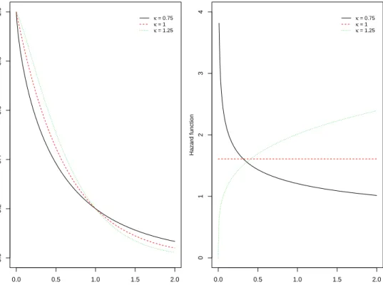
0, κ)0. The parameterκ accommodates a decreasing

(κ < 1), constant (κ = 1) or increasing (κ > 1) hazard; here we focus primarily on the case with κ = 0.75to reflect modest decreasing trend in risk. If the plan is to observe individuals over(0, C†], without loss of generality we let C† = 1 denote the administrative censoring time. The parameter λ0 is then chosen as the solution to P(Tij > C†|Zi = 0) = pa to give the desired administrative censoring rate for the control group, wherepa= 0.2. A random censoring time for thejth individual in clusteriis denoted byC_ij∗ and assumed to be exponentially distributed with rateρ; we assume here thatCij ⊥ Cik|Zi so censoring is independent within clusters. The effective right-censoring time is then Cij = min(Cij∗, C†), and the value ρ that solves P(Tij > Cij|Zi = 0) = p0 gives p0, the net

censoring rate in the control arm; we considerp0 = 0.2to correspond to the case of strictly

admin-istrative censoring and p0 = 0.5to correspond to the case of 30% random and 20% administrative

censoring.

Suppose the within-cluster association in the failure time is induced by the Clayton copula with pa-rameterφ, so the joint survivor function forTi = (Ti1, . . . , TiJ)

0

is given by (2.6), whereJis the clus-ter size. The copula parameclus-ter is chosen to give Kendall’sτ of0.05,0.1, and0.25for small, mild and moderate within-cluster associations, respectively. We consider cluster sizes ofJ = 2, 5, 20, and100

that represent from small to large cluster sizes. For each parameter combination, we compute the re-quired number of clusters (n) on the basis of (2.7) to give power1−γ2 = 0.8using a two-sided test

with a type I error rateγ1 = 0.05. We then generate the corresponding clustered event times and

by Lee et al. [12] to test the null hypothesis of no treatment effect. We report empirical standard error (ESE) and average robust standard error (ASE) forβˆ, empirical rejection rate (REJ%) defined as the percentage of samples in which the null hypothesisH0 : β = 0is rejected by a two-sided Wald test

at the nominal5%level, and the empirical coverage probability (ECP%) of nominal 95% confidence intervals for β (the proportion of simulated samples for which the nominal 95% confidence interval contained the true value ofβ). Because the ECP% is the complement of the REJ% when β = 0, we do not report it in this case; see Table 1.

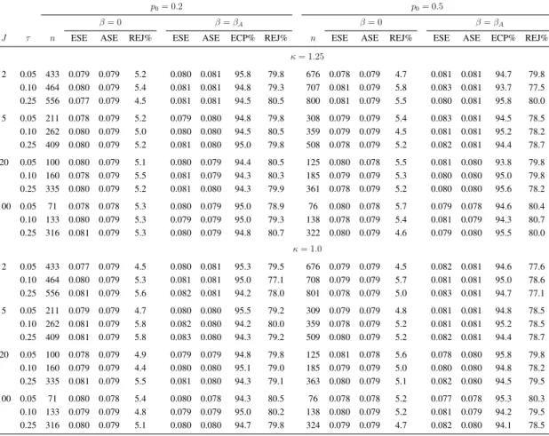
For each parameter configuration we generate 2000 samples, so the half-width of a 95% confi-dence interval for the type I error rate would be approximately1.96(0.05×0.95/2000)1/2 = 0.01, and one could expect the REJ% to fall outside the range[0.04,0.06]in one out of 20 settings by chance; by similar arguments, one would expect the ECP% to fall within the range 94 and 96% 19 times out of 20. If the nominal power 0.80 is correct, then the empirical power would be expected to fall outside the range [0.78,0.82] for one out of every 20 configurations. From Table 1, it is apparent that the REJ% underβ = 0are within the acceptable range for most cases. Under the alternative hypothesis, the empirical coverage probabilities are within the acceptable range of 94-96%, and the REJ% are broadly compatible with the nominal level. All of these findings support the validity of the derived sample size formula. Similar results are seen when the baseline hazard is increasing (κ = 1.25) or constant (κ= 1.0); see Section S2 of the Supporting information.

3

A

C

I

D

R

R

E

3.1 ROBUSTNESS OFPOWER TOMISSPECIFICATION OF THE COPULA FUNCTION

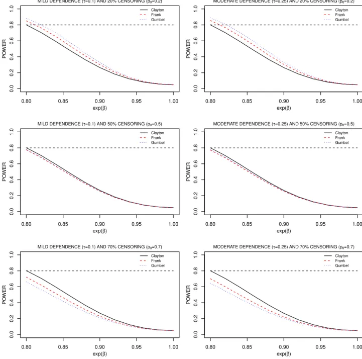
Choosing a suitable copula at the design stage is challenging, so here we explore the sensitivity of study power to misspecified copula functions. We consider the same parameter configurations as in Section 2, where κ = 0.75 and the administrative censoring rate is pa = 0.2. The sample size is estimated under the Clayton copula with Kendall’s τ = 0.1 and 0.25 with βA = log 0.8. Under the derived number of clusters, we construct the corresponding power curves under the Frank or Gumbel copula functions with the same value of Kendall’sτ. Figure 1 shows these power curves for different copula functions forJ = 20under different net censoring rates (p0 = 0.2,0.5and0.7) in the

control arm. When the censoring rate is mild and due strictly to administrative censoring (p0 = 0.2),

misspecification of the copula function impacts power, but use of the Clayton copula ensures power is maintained under the Frank or Gumbel copula functions. When the net censoring rate increases to 50%, the impact of copula misspecification is negligible, however, when the net censoring rate increases to 70%, the impact on power is again appreciable; in this case, the Clayton copula leads to samples sizes which are too small. These findings suggest that the misspecification of copula functions can have significant impact on study power and the impact depends on the censoring rate. The findings are broadly similar for cluster sizes ofJ = 2,5and100.

To examine the effect of copula misspecification more fully we next consider the asymptotic relative efficiencies of the estimators through the functions

AREF:C = asvarF( ˆβ) asvarC( ˆβ) , AREG:C = asvarG( ˆβ) asvarC( ˆβ) , and AREF:G= asvarF( ˆβ) asvarG( ˆβ) , (3.1)

where asvar() denotes an asymptotic variance and ‘C’, ‘F’, and ‘G’ denote the Clayton, Frank and Gumbel copulas, respectively. We setκ = 0.75and β = log 0.8and set the control administrative censoring rate to pa = 0.2 at C† = 1; again λ0 is found to satisfy P(Tij > C†|Zij = 0) = pa. The random censoring times are assumed to be independently exponentially distributed with rateρ, which is selected to ensure a net censoring rate for the control arm through the constraintP(Tij >

T able 1: Sample size estimation and empirical properties of estimators under cluster -randomized designs when within-cluster association between ev ent times is induced by the Clayton copula; κ = 0 . 75 , βA = log 0 . 8 , pa = 0 . 2 , nsim = 2000 . 20% Censoring ( p0 = 0 . 2 ) 50% Censoring ( p0 = 0 . 5 ) β = 0 β = βA β = 0 β = βA J τ n ESE ASE REJ% ESE ASE ECP% REJ% n ESE ASE REJ% ESE ASE ECP% REJ% 2 0.05 433 0.078 0.079 4.8 0.080 0.081 95.2 80.3 677 0.078 0.079 5.1 0.083 0.081 94.8 78.0 0.10 464 0.080 0.079 5.4 0.081 0.081 95.0 79.0 708 0.078 0.079 4.5 0.080 0.081 95.9 79.0 0.25 556 0.077 0.079 5.1 0.081 0.081 94.2 79.8 803 0.079 0.079 4.8 0.081 0.081 94.5 78.8 5 0.05 211 0.081 0.079 5.2 0.083 0.080 94.1 78.0 309 0.079 0.079 5.3 0.081 0.081 95.0 78.4 0.10 262 0.080 0.079 5.4 0.083 0.080 94.0 79.0 359 0.079 0.079 4.4 0.082 0.081 95.0 79.7 0.25 409 0.080 0.079 5.0 0.079 0.080 94.8 79.2 511 0.081 0.079 5.5 0.081 0.081 94.8 79.1 20 0.05 100 0.080 0.078 5.4 0.080 0.079 95.0 78.3 125 0.080 0.078 5.8 0.082 0.080 94.4 80.2 0.10 160 0.079 0.079 4.9 0.078 0.079 95.2 81.0 185 0.077 0.079 4.7 0.082 0.080 94.5 78.5 0.25 335 0.081 0.079 5.7 0.081 0.080 95.0 81.5 365 0.078 0.079 4.8 0.079 0.080 95.0 81.8 100 0.05 71 0.079 0.078 5.8 0.080 0.078 94.1 81.2 76 0.080 0.078 6.0 0.080 0.078 94.1 80.7 0.10 133 0.079 0.079 4.9 0.081 0.079 94.1 79.0 139 0.079 0.079 4.6 0.080 0.079 94.3 81.6 0.25 316 0.081 0.079 6.0 0.080 0.080 94.9 80.0 326 0.081 0.079 5.8 0.080 0.080 95.3 79.8

0.80 0.85 0.90 0.95 1.00 0.0 0.2 0.4 0.6 0.8 1.0 exp(β) PO WER

MILD DEPENDENCE (τ=0.1) AND 20% CENSORING (p0=0.2)

Clayton Frank Gumbel 0.80 0.85 0.90 0.95 1.00 0.0 0.2 0.4 0.6 0.8 1.0 exp(β) PO WER

MODERATE DEPENDENCE (τ=0.25) AND 20% CENSORING (p0=0.2)

Clayton Frank Gumbel 0.80 0.85 0.90 0.95 1.00 0.0 0.2 0.4 0.6 0.8 1.0 exp(β) PO WER

MILD DEPENDENCE (τ=0.1) AND 50% CENSORING (p0=0.5)

Clayton Frank Gumbel 0.80 0.85 0.90 0.95 1.00 0.0 0.2 0.4 0.6 0.8 1.0 exp(β) PO WER

MODERATE DEPENDENCE (τ=0.25) AND 50% CENSORING (p0=0.5)

Clayton Frank Gumbel 0.80 0.85 0.90 0.95 1.00 0.0 0.2 0.4 0.6 0.8 1.0 exp(β) PO WER

MILD DEPENDENCE (τ=0.1) AND 70% CENSORING (p0=0.7)

Clayton Frank Gumbel 0.80 0.85 0.90 0.95 1.00 0.0 0.2 0.4 0.6 0.8 1.0 exp(β) PO WER

MODERATE DEPENDENCE (τ=0.25) AND 70% CENSORING (p0=0.7)

Clayton Frank Gumbel

Figure 1: Power curves for different copula functions when sample size is estimated on the basis of the the Clayton copula withτ = 0.10(left column) andτ = 0.25(right column) under 20% (top row), 50% (middle row) and 70% (bottom row) net censoring for the control arm;κ= 0.75, βA= log 0.8,

Cij|Zi = 0) = p0, where p0 ranges from 0.2 to 0.8. Figure 2 displays the contour plots of the

asymptotic relative efficiencies in (3.1) as a function of the degree of within-cluster association in the event times (Kendall’sτ) and the net censoring rate (p0) for bothJ = 20 (left panels) andJ = 100

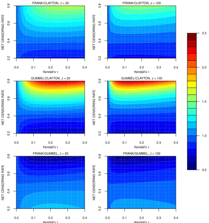
(right panels); we restrict attention to values of Kendall’s τ ranging from 0 to 0.4 to cover realistic scenarios. ForJ = 20, if the net censoring rate is less than 40%, the Gumbel copula leads to a more efficient estimator, followed by the Frank copula and then the Clayton copula; the Clayton copula should therefore be used for the sample size calculations to ensure adequate power among this set of copulas. If the net censoring rate in this setting is higher than 40-50%, the Gumbel copula should be adopted at the design stage since it yields the estimator with the greater variance. The trend is broadly similar forJ = 100. 0.0 0.1 0.2 0.3 0.4 0.2 0.4 0.6 0.8 Kendall’s τ NET CENSORING RA TE FRANK/CLAYTON, J = 20 0.0 0.1 0.2 0.3 0.4 0.2 0.4 0.6 0.8 Kendall’s τ NET CENSORING RA TE FRANK/CLAYTON, J = 100 0.0 0.1 0.2 0.3 0.4 0.2 0.4 0.6 0.8 Kendall’s τ NET CENSORING RA TE GUMBEL/CLAYTON, J = 20 0.0 0.1 0.2 0.3 0.4 0.2 0.4 0.6 0.8 Kendall’s τ NET CENSORING RA TE GUMBEL/CLAYTON, J = 100 0.0 0.1 0.2 0.3 0.4 0.2 0.4 0.6 0.8 Kendall’s τ NET CENSORING RA TE FRANK/GUMBEL, J = 20 0.0 0.1 0.2 0.3 0.4 0.2 0.4 0.6 0.8 Kendall’s τ NET CENSORING RA TE FRANK/GUMBEL, J = 100 0.5 1.0 1.5 2.0 2.5

Figure 2: Contour plots of the asymptotic relative efficiencies in (3.1) for estimators defined as the solution to (2.2) when clustered failure times are generated on the basis of different copula functions; κ= 0.75,β = log 0.8,pa = 0.2.

is sensitive to both the copula function and censoring rate. A simple pragmatic approach to deal with this sensitivity is to consider a class of copula functions and a range of administrative and random censoring rates. The required sample sizes can be computed for each configuration by (2.7), and the largest sample size can then be chosen to ensure the pre-specified power requirements are met for any copula model and censoring pattern among those considered. Of course there may also be uncertainty in the value of Kendall’s τ, but in this case the largest plausible value of τ will lead to the largest sample size within a given copula family and at a given censoring rate.

3.2 IMPACT OFWITHIN-CLUSTERDEPENDENCE IN THE RANDOMCENSORINGTIMES

Although the assumption of independent censoring times within clusters is commonly, the factors inducing the association in the failure times within clusters may also induce an association in the censoring times. Here we examine the impact of within-cluster dependence in the censoring times on study power. We consider a trial designed to have 80% power to detectβ = log 0.8on the basis of a two-sided Wald test at the 5% significance level under the assumption that random censoring times are independent within clusters and a Clayton copula model is used for the response. In this case, the minimal required sample size is estimated under the within-cluster independent censoring assumption (2.7) in which (A.13) is used to computeB. We then calculate the theoretical power when the within-cluster censoring times are correlated, and (A.9) is used to computeB. We letκ = 0.75, pa = 0.2, and consider J = 2 and J = 20 with net censoring rates ranging from 0.2 to 0.8. The Clayton, Frank and Gumbel copula functions are considered for jointly modeling the distribution of the censoring times within clusters. While it is more general to allow different degrees of within-cluster associations for the failure and censoring times, for parsimony we restrict attention to the case that the value of Kendall’sτ is the same for the failure times (τ) and censoring times (τc).

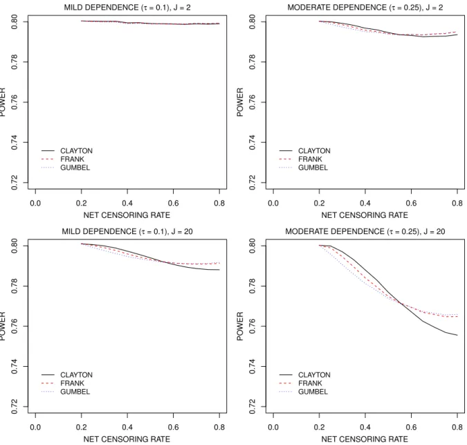
Figure 3 suggests that the naive assumption of within-cluster independence in the censoring times can lead to sample sizes which are too small and hence studies with inadequate power. As the net censoring rate increases (and hence the proportion of event times censored by the random censoring time increases) this effect becomes more pronounced. For example, forJ = 20 andτ = 0.25, the power is0.8for all the copula functions whenp0 = 0.2as in this case there is no dependent random

censoring time. However, when the net censoring rate increases to 80%, the power decreases to 0.756, 0.765 and 0.766 under the Clayton, Frank and Gumbel copula models for the censoring times. Further, if we compare the left panel to the right panels of Figure 3, we find that when the association in the censoring times increases, the power implications of ignoring the within-cluster dependence become more serious for all copula functions. The power is also more seriously impacted with larger cluster sizes; compare the top panels to the respective bottom panels of Figure 3.

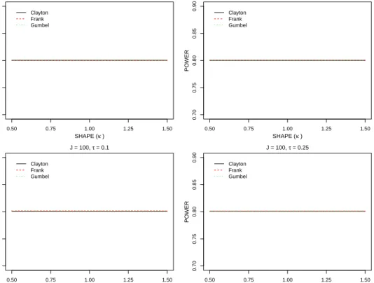
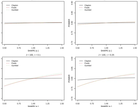
A reviewer suggested examining the effect of misspecifying the shape of the baseline hazard function in the marginal event time distribution in the setting where the administrative and random censoring rates are correct; this ensures that the expected number of events is comparable in the assumed and true parameter settings but would mean, naturally, that the times of the events would be misspecified. The details on how this was investigated, along with the associated findings, are given in Section S3 of the Supporting information. We find that there is negligible impact on power of misspecifying the shape parameter in this setting when there is only administrative censoring. When the event times are subject to random censoring, there can be an increase or decrease in the power compared to the nominal level, and the extent of the effect depends on the copula function modeling the within-cluster dependence; this is not surprising as it is well known that the different copula functions model the association between event times differently over the range of possible values.

0.0 0.2 0.4 0.6 0.8 0.72 0.74 0.76 0.78 0.80

NET CENSORING RATE

PO WER MILD DEPENDENCE (τ = 0.1), J = 2 CLAYTON FRANK GUMBEL 0.0 0.2 0.4 0.6 0.8 0.72 0.74 0.76 0.78 0.80

NET CENSORING RATE

PO WER MODERATE DEPENDENCE (τ = 0.25), J = 2 CLAYTON FRANK GUMBEL 0.0 0.2 0.4 0.6 0.8 0.72 0.74 0.76 0.78 0.80

NET CENSORING RATE

PO WER MILD DEPENDENCE (τ = 0.1), J = 20 CLAYTON FRANK GUMBEL 0.0 0.2 0.4 0.6 0.8 0.72 0.74 0.76 0.78 0.80

NET CENSORING RATE

PO WER MODERATE DEPENDENCE (τ = 0.25), J = 20 CLAYTON FRANK GUMBEL

Figure 3: Power implications of within-cluster association in the random censoring times under joint censoring models induced by different copula functions where the within-cluster association in the failure and censoring times are constrained to be the same (τ =τc); the original sample size is com-puted on the basis of a Clayton copula model for the failure times and the assumption of independent censoring times;κ= 0.75, βA= log 0.8,p0 = 0.2.

4

S

S

C

T

C

I

-C

E

T

4.1 ESTIMATING EQUATIONS AND SAMPLESIZECRITERIA

Interval-censored event times arise when it is only possible to determine whether events have occurred at periodic assessments [36]. In rheumatology studies, for example, interest lies in the time to the development of joint damage, but the extent of joint damage is only possible to determine when patients undergo radiographic examination [37]. In this case the time of joint damage will only be known to fall between the time of the first radiograph showing evidence of damage and the time of the preceding radiographic examination. Other examples include trials aiming to evaluate osteoporosis treatments for the prevention of asymptomatic fractures, studies of the development of new metastatic lesions, and studies in nephrology on the development of kidney stones.

We assume again that Tij|Zi follows a proportional hazards model (2.1) with a q×1parameter

α indexing the baseline hazard and β the regression parameter of interest. The marginal survivor function F(t|Zi;θ) = P(Tij ≥ t|Zi;θ) is then indexed by a (q + 1)×1 parameter θ = (α0, β)0. In the present setting, we consider a cluster-randomized trial in which the plan is to observe each individual atR prespecified assessment timesa1, . . . , aR; we leta0 = 0 andaR+1 =∞. Under this

observation scheme, we observeYijr = I(ar−1 < Tij ≤ ar), r = 1, . . . , R+ 1. The response data provided by individual j in cluster iisYij = (Yij1, . . . , YijR)0, whereYij,R+1 = 1−

PR

r=1Yijr, and

Yi = (Yi01, . . . , YiJ0 )0contains all response data from clusteri,i= 1, . . . , n. Letµij = (µij1, . . . , µijR)0, where µijr =E[Yijr|Zi;θ] =P(ar−1 < Tij ≤ar|Zi;θ) =F(ar−1|Zi;θ)− F(ar|Zi;θ), r = 1, . . . , R. Let µi = (µ0i1, . . . , µ 0 iJ) 0

denote a J R×1 vector and Di = [∂µi/∂α0, ∂µi/∂β] aJ R×(q+ 1) matrix of associated derivatives. We consider the generalized estimating equations for θ, similar to those of Kor et al. [38],

U(θ) = n X i=1 Ui(θ) = n X i=1 Ui(α) Ui(β) = n X i=1 D0_iV_i−1(Yi−µi). (4.1)

where Vi is a J R×J R working covariance matrix. A working independence assumption is par-ticularly convenient in this context, and provided robust variance estimates are used at the time of analysis, inferences can be valid when there is within-cluster dependence in the event times. In this caseVi is block diagonal with R×Rblock diagonal matrices Vij =Cov(Yij, Yij0|Zi),j = 1, . . . , J, which account for the correlation of responses at different assessment times within individuals; that is, Vi =    Vi1 . .. ViJ   =     Cov(Yi1, Yi01|Zi)

0

0

and the(r, s)th entry ofVij is

Cov(Yijr, Yijs|Zi) =

µijr(1−µijr), r=s; −µijrµijs, r6=s .

(4.3)

Note that if the marginal regression models are correctly specified, n−1/2_{U(θ)is asymptotically}

multivariate normal with mean zero and covariance given analogously to (2.3) by

estimated as b B = 1 n n X i=1 Ui(θ)Ui0(θ) θ=bθ .

The estimator bθ is the root of U(θ) = 0 and is consistent for θ with n1/2(θb− θ)

D

−→ N(0,Γ)

asymptotically, where Γ = A−1_B[A−1_]0

, and A = −E[∂Ui(θ)/∂θ0]. Again the matrix A can be consistently estimated by b A=−1 n n X i=1 ∂Ui(θ)/∂θ0 θ=θb . (4.5)

Model assumptions are required to derive the sample size formula on the basis of the preceding asymptotic variance formula for clustered interval-censored data. Copula functions can be used to construct the joint distribution with any specified marginal properties. Consider a cluster-randomized trial in which the treatment is randomly allocated to clusters. Suppose we aim to test whether the treatment has an effect on the time to a certain event. The null hypothesis isH0 : β = β0 = 0, and

the alternative hypothesis isHA: β6=β0, and letβAdenote the clinically important effect.

As in Section 2, the limiting distribution of a Wald statistic can be used to select the required sample size (number of clusters) for a two-sided test with significance levelγ1 and power1−γ2. The

key point is to derive the formulae forA =E[−∂Ui(θ)/∂θ0]andB = E[Ui(θ)Ui0(θ)], and hence the form ofΓ = A−1_B[A−1_]0

, so the required sample size can be obtained on the basis ofΨ = Γq+1,q+1,

the element from the covariance matrix; the formulae are outlined in Appendix B. The resulting sample sizennecessary to detect the effect of treatment with the specified power is

n ≥ _z γ1/2 √ Ψ0+zγ2 √ ΨA βA 2 , (4.6)

where Ψ0 and ΨA are the elements of Γ computed under the null and alternative settings. At the design stage of clinical trials, to estimate the required number of clusters, specifications of the effect of interest βA, cluster sizeJ, inspection times a1, . . . , aR, parametric baseline hazard function, and especially the joint distribution for clustered event times are required.

4.2 EMPIRICALVALIDATION OFSAMPLESIZEFORMULA FORCLUSTEREDINTERVAL-CENSORED

EVENT TIMES

Here we examine the performance of the proposed sample size formula for clustered interval-censored data. Consider an equal allocation cluster-randomized trial with binary treatment covariateZi,P(Zi =

1) = P(Zi = 0) = 0.5. Assume that Tij follows the proportional hazards model given by (2.1) with Weibull baseline cumulative hazard Λ0(s) = (λ0s)κ, where α = (logλ0,logκ)0, q = 2, and

θ = (α0, β)0, j = 1, . . . , J, i = 1, . . . , n; we consider cluster sizes ofJ = 2, 5, 20 and 100. Sup-pose κ = 0.75 and choose λ0 so that P(Tij > 1|Zi = 0) = pa to give a specified administrative censoring rate; we set pa = 0.2. Suppose the plan is to assess each individual R times over the in-terval [0,1]at prespecified assessment timesa1, . . . , aR evenly spaced over the observation interval, that is,ar = r/R, r = 1, . . . , R, withR = 2, 4 or 12. LetYij = (Yij1, . . . , YijR)

0

denote the event information provided by individualj in clusteri, whereYijr =I(ar−1 < Tij ≤ar).

Suppose the within-cluster association in the underlying failure times is induced by the Clayton copula with Kendall’sτ of 0.05, 0.10, and 0.25 for small, mild and moderate within-cluster associa-tion respectively. For each parameter combinaassocia-tion, we estimate the sample size (number of clusters) by (4.6) given βA = log 0.8, the type I error rate γ1 = 0.05 and power 1−γ2 = 0.8. After

responseYi. Parameter estimate are then obtained via the estimating equation (4.1). For each param-eter combination, nsim = 2000datasets are simulated and analysed to yield 2000 estimates ofβ and respective robust variance estimates. The ESE, ASE, REJ%and95%ECP%are summarized in Table 2.

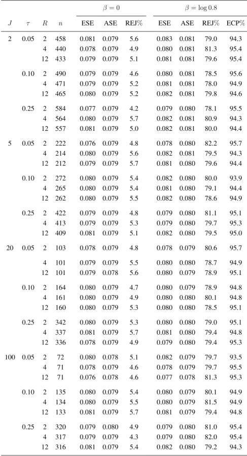
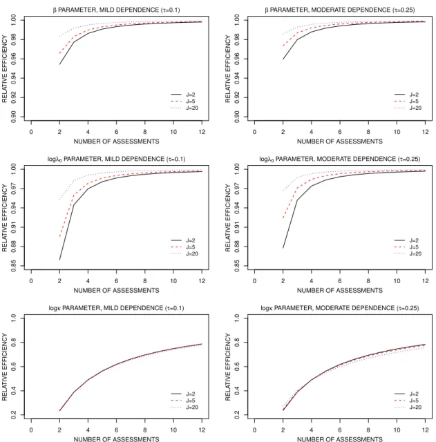
The REJ% is close to the nominal type I error rate whenβ = 0and close to the nominal power whenβ = log 0.8, with the latter supporting the validity of the sample size formula. The empirical biases (not shown) are all negligible, so it is not surprising that the empirical coverage probabilities are all compatible with the nominal 95% level. As the number of assessments increases, the required sample size is found to decrease, but the extent of this decrease from the case ofR = 4toR = 12is quite small, particularly when cluster sizes are large. To clearly understand the impact of the number of assessments on the efficiency, we computed the asymptotic relative efficiency of estimators for the marginal parameters, defined as

AREr,k=

asvar(˜θk) asvarr(ˆθk)

,

where asvar(˜θk)is the asymptotic variance ofθkforR= 100; this value is large enough to mimic the case that the event times are known precisely, that is, the case of clustered right-censored event times. The term asvarr(ˆθk)represents the asymptotic variance of θb_k for the caseR = r, corresponding to clustered interval-censored failure time data, wherek = 1,2,3.

Figure 4 shows the trend of asymptotic relative efficiency for estimators of the marginal param-eters with cluster sizes ofJ = 2, 5, and 20, respectively. From these figures, we note that when the number of assessments increases to R = 8, the asymptotic relative efficiencies for both λ0 and β

are close to 1 in all cases considered. This also supports the empirical findings that the number of clusters required decreases very little when the number of assessments increases fromR = 4to12. Figure 4 also shows that the impact of the number of assessments is more severe for small cluster sizes, which agrees with what we found from Table 2. As one might expect, however, the number of assessments seriously affects the efficiency of the estimator for the trend parameter κ, so when the entire marginal distribution is of interest, increasing the number of assessments certainly can improve efficiency for some features of the distribution. There is of course a trade-off between the statistical goals of precision and power and the economic and other costs. The development of optimal design criteria which enables one to weigh the merits of increasing the number of clusters or the number of follow-up assessments to be scheduled, subject to prespecified budgetary constraints, represents an important area of future research.

5

I

E

I

T

O

M

Otitis media is inflammation of the inner ear which puts patients at risk of permanent damage and loss of hearing. We illustrate the steps in trial design by considering the study discussed in Manatunga and Chen [14] in which children from 6 months to 8 years of age with otitis media requiring surgical insertion of tubes in the auditory canal are randomized to receive either 2 weeks of medical therapy with prednisone and sulfamethoprim or no medical therapy (standard care). The trial is conceived on the basis of the data in Le and Lindgren [13] in which all children except one had bilateral inflam-mation, and so we consider clusters of size two withJ = 2. In the absence of information on the trend, we setκ = 1. The median time to failure of the inserted tube was estimated to be 7 months, assuming 30 days per month yieldsλ0 =−log 0.5/210 ≈ 0.0033. As in Manatunga and Chen [14]

we set τ = 0.56 to reflect moderate to strong within-child association in the failure times. Since follow-up is planned for 1.5 years, we set C† = 540 and anticipate an administrative censoring rate of 17% for the control arm. To accommodate study withdrawal, we adopt an exponential model for

Table 2: Sample size estimation and empirical properties of estimator βˆ under cluster-randomized design for interval-censored data when the Clayton copula is used to induce the within-cluster asso-ciation between event times;κ= 0.75,βA = log 0.8,pa = 0.2, nsim= 2000.

β= 0 β= log 0.8

J τ R n ESE ASE REJ% ESE ASE REJ% ECP%

2 0.05 2 458 0.081 0.079 5.6 0.083 0.081 79.0 94.3 4 440 0.078 0.079 4.9 0.080 0.081 81.3 95.4 12 433 0.079 0.079 5.1 0.081 0.081 79.6 95.4 0.10 2 490 0.079 0.079 4.6 0.080 0.081 78.5 95.6 4 471 0.079 0.079 5.2 0.081 0.081 78.0 94.9 12 465 0.080 0.079 5.2 0.082 0.081 79.8 94.6 0.25 2 584 0.077 0.079 4.2 0.079 0.080 78.1 95.5 4 564 0.080 0.079 5.7 0.082 0.081 80.9 94.3 12 557 0.081 0.079 5.0 0.082 0.081 80.0 94.4 5 0.05 2 222 0.076 0.079 4.8 0.078 0.080 82.2 95.7 4 214 0.080 0.079 5.6 0.082 0.081 79.5 94.3 12 212 0.079 0.079 5.7 0.081 0.080 79.6 94.4 0.10 2 272 0.080 0.079 5.4 0.082 0.080 80.0 93.9 4 265 0.080 0.079 5.4 0.081 0.080 79.1 94.4 12 262 0.080 0.079 5.5 0.082 0.080 78.6 94.9 0.25 2 422 0.079 0.079 4.8 0.079 0.080 81.1 95.1 4 413 0.079 0.079 5.3 0.079 0.080 79.7 95.3 12 409 0.081 0.079 5.1 0.082 0.080 79.5 95.0 20 0.05 2 103 0.078 0.079 4.8 0.078 0.079 80.6 95.7 4 101 0.079 0.079 5.5 0.080 0.080 78.7 94.9 12 101 0.079 0.078 5.6 0.080 0.079 78.9 95.1 0.10 2 164 0.080 0.079 4.7 0.080 0.079 78.9 94.8 4 161 0.080 0.079 4.9 0.080 0.080 80.1 94.8 12 160 0.080 0.079 5.3 0.080 0.080 78.5 95.1 0.25 2 342 0.080 0.079 5.3 0.080 0.080 79.0 95.1 4 337 0.081 0.079 5.7 0.081 0.080 79.4 94.8 12 336 0.078 0.079 4.9 0.079 0.080 79.4 95.3 100 0.05 2 72 0.080 0.078 5.1 0.082 0.079 79.7 93.5 4 71 0.078 0.079 4.6 0.078 0.079 79.7 95.5 12 71 0.076 0.078 4.6 0.077 0.078 81.3 95.3 0.10 2 135 0.080 0.079 5.4 0.080 0.079 80.1 94.9 4 134 0.080 0.079 5.5 0.080 0.079 81.5 94.9 12 133 0.081 0.079 5.7 0.081 0.079 79.4 94.8 0.25 2 320 0.079 0.080 4.9 0.079 0.080 81.0 95.4 4 317 0.079 0.079 4.3 0.079 0.080 82.0 95.4 12 316 0.081 0.079 5.4 0.082 0.080 79.2 94.3

0 2 4 6 8 10 12 0.90 0.92 0.94 0.96 0.98 1.00 NUMBER OF ASSESSMENTS RELA TIVE EFFICIENCY

β PARAMETER, MILD DEPENDENCE (τ=0.1)

J=2 J=5 J=20 0 2 4 6 8 10 12 0.90 0.92 0.94 0.96 0.98 1.00 NUMBER OF ASSESSMENTS RELA TIVE EFFICIENCY

β PARAMETER, MODERATE DEPENDENCE (τ=0.25)

J=2 J=5 J=20 0 2 4 6 8 10 12 0.85 0.88 0.91 0.94 0.97 1.00 NUMBER OF ASSESSMENTS RELA TIVE EFFICIENCY

logλ0 PARAMETER, MILD DEPENDENCE (τ=0.1)

J=2 J=5 J=20 0 2 4 6 8 10 12 0.85 0.88 0.91 0.94 0.97 1.00 NUMBER OF ASSESSMENTS RELA TIVE EFFICIENCY

logλ0 PARAMETER, MODERATE DEPENDENCE (τ=0.25)

J=2 J=5 J=20 0 2 4 6 8 10 12 0.2 0.4 0.6 0.8 1.0 NUMBER OF ASSESSMENTS RELA TIVE EFFICIENCY

logκ PARAMETER, MILD DEPENDENCE (τ=0.1)

J=2 J=5 J=20 0 2 4 6 8 10 12 0.2 0.4 0.6 0.8 1.0 NUMBER OF ASSESSMENTS RELA TIVE EFFICIENCY

logκ PARAMETER, MODERATE DEPENDENCE (τ=0.25)

J=2 J=5 J=20

Figure 4: Asymptotic relative efficiency of estimators for marginal parameters for clustered interval-censored event times as a function of the number of assessments, degree of dependence and copula function.

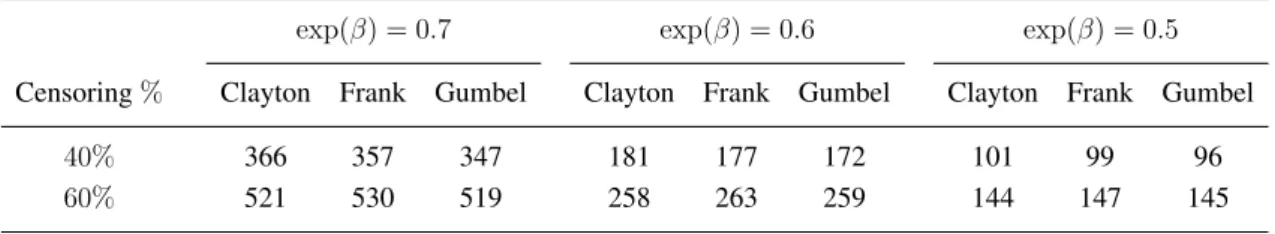
loss to follow-up to give a net rate of censoring in the control arm of 40% or 60%. Note that this setting is slightly different than the setting discussed in Section 3 where different individuals within each cluster had different censoring times; here the clusters are defined by children and the times to failure of the left and right tubes would be censored at a common time. The formula in Appendix A can be easily modified to address this by definingG˜(·)as the survival distribution for the cluster-level censoring time and replacing G(s, t)by G˜(max(s, t))in (A.9). Under Clayton, Frank and Gumbel copulas, we compute the number of children required to randomize to ensure 80% power to detect a 30, 40 or 50% reduction in the marginal hazard for failure based on a two-sided test at the 5% level. The results displayed in Table 3 provide a simple illustration of how the most conservative copula depends on the rate of censoring. When the net censoring is expected to be 40%, the Clayton copula yields the largest sample size, but when it is 60%, the Frank copula yields the largest sample sizes.

Table 3: Number of clusters (children) required for otitis media study under Clayton, Frank and Gumbel copulas for different clinically important treatment effects and net censoring rates.

exp(β) = 0.7 exp(β) = 0.6 exp(β) = 0.5

Censoring% Clayton Frank Gumbel Clayton Frank Gumbel Clayton Frank Gumbel

40% 366 357 347 181 177 172 101 99 96

60% 521 530 519 258 263 259 144 147 145

6

D

We derived sample size formulae for cluster-randomized trials involving right- and interval-censored event times in which the analysis is based on a marginal proportional hazards assumption. For right-censored data, we derived expressions for the asymptotic robust variance of the Wald statistic on the basis of the approach of Lee et al. [12], and for clustered interval-censored data, we likewise adopted the structure of Kor et al. [38]. Both of these frameworks invoke a working independence assumption, so robust variance estimation is required to ensure valid inference in the presence of within-cluster as-sociation. The simulation studies conducted confirm that the formulae are valid. Code for computing the required sample size is available in R from the authors upon request. Robustness of these formulae to the misspecification of copula functions and to within-cluster dependence in the censoring times is also investigated using large sample theory for clustered failure times in the context of right-censored data.

As in other sample size formula for cluster-randomized trials, the derived formulae require speci-fication of the degree of within-cluster dependence, measured in the failure time setting by Kendall’s τ. A good approximation to the degree of within-cluster dependence is important [39], so it is there-fore customary to rely on estimates reported in the literature. We recognize that it is unlikely that values of Kendall’sτ would be reported in the clinical literature, and so we recommend the conduct of small pilot studies. More recently, there has been increased interest in planning trials with adaptive sample size re-estimation. This is carried out in its simplest form by having an internal pilot study, after which blinded data are used to estimate unknown parameters; these new estimates are then used to revise sample size calculations. This is a generally important area of research as these methods increase efficiency. We have developed such methods in another context [40] and plan to study this in the present setting in future work.

We have focussed on settings with a single binary treatment indicator, but the proposed meth-ods extend naturally to deal with trials where analyses control for cluster-level covariates. A

two-dimensional covariate vector would arise if one designed a three-armed trial, in which case one might specify Zi = (Zi1, Zi2)0 where Zi1 andZi2 indicate assignment to the first and second

experimen-tal treatments, respectively, and Zi1 = Zi2 = 0 if cluster i is assigned to the control intervention.

More generally, other multidimensional descriptive cluster-level covariates can be incorporated into the analyses, but at the design stage their joint distribution would have to be specified to facilitate computation of the matrix expectations in the robust variance formula; see Appendices A and B. Individual-level covariates can also be controlled for in the analysis in principle, but assumptions would again be required regarding their joint distribution and in particular the extent to which these covariates are dependent within clusters.

We also restricted attention to the setting in which cluster sizes are fixed at a common value, denoted by J. While this is often reasonable, cluster sizes routinely vary within studies. When planning studies in this case, it is perhaps most common to use formulae derived for fixed cluster sizes but to use the anticipated average cluster sizeJ¯=Pn

i=1Ji/nin the formula in place ofJ[29, 32, 41].

When cluster sizes vary and the response is continuous, use of the average size in the formula derived for common cluster sizes can lead to inadequate power; the loss in power can be small, however, if the cluster size tends to be large and the intraclass correlation coefficient is small [42, 43]. Manatunga et al. [42] developed a refinement to the usual sample size formula for continuous outcomes to deal with variable cluster sizes, which involves adding a correction term (a function of the coefficient of variation of the cluster size) to the formula on the basis of a common cluster size. Van Breukelen et al. [43] investigated the consequences of unequal versus equal cluster sizes in terms of the precision of treatment effects estimators in cluster-randomized trials with continuous outcomes. They provide a formula for the approximate relative efficiency of the estimators, which can be used to adjust an initial estimate of the number of clusters required on the basis of a common cluster size. Candel and Van Breukelen [44] extended this approach to varying cluster size with binary outcomes when the analysis is based on the mixed logistic regression. We are not aware of any methods for dealing with variable cluster sizes for event time responses, and so extensions to deal with this represent an important area of future research.

In principle, the methods we develop can be adapted to the setting in which the number of clusters is fixed, and the goal is to determine the number of individuals within each cluster necessary to achieve the desired power. This may be a more appropriate framework in a health promotion study, for example, in which clinics are randomized to deliver one of two smoking cessation programs. If there are a fixed number of clinics available to take part but patients are continually being referred to these clinics, it is natural to want to know how many patients should be recruited from these clinics to ensure adequate power to detect a specified effect of an experimental cessation program. As pointed out by Hemming et al. [45], the limiting robust standard deviation of estimators obtained under the working independence assumption decreases as the cluster size increases, but there is a positive limiting value. As a result, for a given number of clusters, minimal clinically important effect, and type I error rate, there is a limit to the power that can be achieved by increasing the cluster size. Conversely, for a given number of clusters, power, and type I error rate, there is a limit to how small the effect can even as cluster sizes increase. In situations where small clinically important effects are specified, it may therefore be necessary to select the number of clusters and the cluster size in concert to ensure practical and statistical constraints are met.

When the clustered event times are interval-censored data, our sample size formula is derived based on the assumption that all the assessments on each individual are available. Individuals may of course prematurely drop-out of studies, leading to missed assessments. In this case, the response vectors are incompletely observed, but modifications to the estimating functions are straightforward if assumptions about the withdrawal process are made.

A

A

L

D

W

S

C

R

-C

E

T

In what follows, we consider the setting in which Zi is a fixed binary treatment indicator and as-sume that the marginal distribution of Tij, the event time for individualj in cluster i, satisfies the proportional hazard assumption with

λij(t|Zi) =λ0(t;α) exp(Ziβ),

whereλ0(t;α)is the baseline hazard function indexed by a vectorα, aβ is the coefficient of interest,

andj = 1, . . . , J,i= 1, . . . , n. IfC†is an administrative censoring time, the plan is to observe over

(0, C†], butC_ij∗ is a random censoring time with survivor functionG∗_{(c), representing a possible early}

withdrawal time. The net censoring time for individualj in clusteriis thenCij =min(Cij∗, C

†₎

, with survivor functionG(c).

In counting process notation, we let{Nij(t),0< t}denote the right-continuous counting process forTij, whereNij(t) = I(Tij ≤ t)indicates that the event occurred at or before timetfor individual

j in cluster i. Then dNij(t) = 1 if individual j in cluster i experiences the event at time t, and

dNij(t) = 0otherwise. LetY¯ij(t) =Yij(t)Y

†

ij(t)be the indicator that thejth individual in clusteriis under observation and at risk of event at timet, whereY_ij†(t) =I(Tij ≥t)andYij(t) =I(Cij ≥t).

Under working independence assumption, the partial score function forβ is

U(β) = n X i=1 J X j=1 Z ∞ 0 ¯ Yij(t) Zi− PJ j=1S1j(t;β) PJ j=1S0j(t;β) ! dNij(t),

where Srj(t;β) = n−1Pn_i=1Y¯ij(t)Zirexp(Ziβ), r = 0,1 and Zi0 = 1 and Zi1 = Zi. Lee et al. [12] show that the score function is asymptotically equivalent to a sum of independent identically distributed terms n−1/2U(β) =n−1/2 n X i=1 J X j=1 ζij where ζij = Z ∞ 0 ¯ Yij(t)(Zi−W(t))dMij(t), where we suppress the functional dependence onβin the termsW(t) =PJ

j=1s1j(t;β)/

PJ

j=1s0j(t;β)

withsrj(t;β)the limit ofSrj(t;β), and

Mij(t) =Nij(t)−

Z t

0

¯

Yij(u) exp(Ziβ)λ0(u)du

where {Mij(t),0 < t} is a martingale. By the Central Limit Theorem, n−1/2U(β)converges to a normal random variable with mean0and varianceB, where

B=n−1 n X i=1 Var(ζi·) = J X j,k=1 Cov(ζij, ζik) = J X j,k=1 E(ζijζik), (A.1) whereζi· =PJ_j=1ζij,i= 1, . . . , n.

The root ofU(β) = 0is a consistent estimatorβbwithn1/2(βb−β)

D

−→N(0,Γ), whereΓ =B/A2

andA =−E[∂Ui(β)/∂β]. The sample size formula is derived on the basis of this limiting distribution with theBandAcomputed on the basis of parametric models. We give the results of these derivations in the following two sections under the assumption of dependent within-cluster censoring times and independent censoring within clusters.

A.1 GENEARL DERIVATION OFB

We first consider a general case in which the censoring times could be correlated within clusters. Assume(Ci1, . . . , CiJ)0 ⊥ Zi and letG(u) = P(Cij ≥u)be the survivor function for the censoring time Cij, and G(s, t) = P(Cij ≥ s, Cik ≥ t) denote the joint survivor function for the censoring times(Cij, Cik)within clusteri; both are assumed common across the two groups. The joint survivor functionG(s, t)describes the association between within-cluster censoring times.

To derive an expression for (A.1) we first consider the case wherej =k and note

Eζ_ij2 =E Z C 0 ¯ Yij(s)(Zi−W(s))2λij(s)ds =EZi E_Y† ij(s)|Zi E_Y ij(s)|Yij†(s),Zi Z C 0 ¯ Yij(s)(Zi−W(s))2λij(s)ds =EZi E_Y† ij(s)|Zi Z C 0 G(s)Y_ij†(s)(Zi−W(s))2λij(s)ds =EZi Z C 0 G(s)P(Tij ≥s|Zi)(Zi−W(s))2λij(s)ds =EZi Z C 0 G(s)(Zi−W(s))2fj(s|Zi)ds (A.2)

where fj(s|Zi)is the conditional density of the event time for individual j in cluster i. AndEZi[·]

depends on the trial allocation probability. Forj 6=k, since E[ζijζik] =E Z Z (0,C]2 ¯ Yij(s) ¯Yik(t)(Zi−W(s))(Zi−W(t))dMij(s)dMik(t) , and dMij(s)dMik(t) = dNij(s)dNik(t)−dNij(s) ¯Yik(t)dΛik(t)−Y¯ij(s)dΛij(s)dNik(t) −Y¯ij(s) ¯Yik(t)dΛij(s)dΛik(t), then E[ζijζik] =E Z Z (0,C]2 ¯ Yij(s) ¯Yik(t)(Zi−W(s))(Zi−W(t))dNij(s)dNik(t) −E Z Z (0,C]2 ¯ Yij(s) ¯Yik(t)(Zi−W(s))(Zi−W(t))dNij(s)dΛik(t) −E Z Z (0,C]2 ¯ Yij(s) ¯Yik(t)(Zi−W(s))(Zi−W(t))dΛij(s)dNik(t) +E Z Z (0,C]2 ¯ Yij(s) ¯Yik(t)(Zi−W(s))(Zi−W(t))dΛij(s)dΛik(t) . (A.3)

The first term in (A.3) is then computed as E " Z Z (0,C]2 ¯ Yij(s) ¯Yik(t)(Zi−W(s))(Zi−W(t))dNij(s)dNik(t) # =EZi h E_Y† ij(s),Y † ik(t)|Zi n E_dN ij(s),dNik(t)|Y † ij(s),Y † ik(t),Zi h E_Y ij(s),Yik(t)|Zi,Yij†(s),Y † ik(t),dNij(s),dNik(t) nZ Z (0,C]2 ¯ Yij(s) ¯Yik(t)(Zi−W(s))(Zi−W(t))dNij(s)dNik(t) oioi =EZi h E_Y† ij(s),Y † ik(t)|Zi n E_dN ij(s),dNik(t)|Yij†(s),Y † ik(t),Zi h Z Z (0,C]2 G(s, t)Y_ij†(s)Y_ik†(t)(Zi−W(s))(Zi−W(t))dNij(s)dNik(t) ioi =EZi h E_Y† ij(s),Y † ik(t)|Zi nZ Z (0,C]2 G(s, t)Y_ij†(s)Y_ik†(t)(Zi−W(s))(Zi−W(t))P(Tij =s, Tik=t|Yij†(s), Y † ik(t), Zi)dsdt oi =EZi hZ Z (0,C]2 G(s, t)(Zi−W(s))(Zi−W(t))fjk(s, t|Zi)dsdt i , (A.4)

wherefjk(s, t|Zi)is the pairwise conditional density for(Tij, Tik)obtained through the specification of a copula function. Using the same strategy for remaining terms of (A.3), we obtain

E Z Z (0,C]2 ¯ Yij(s) ¯Yik(t)(Zi−W(s))(Zi−W(t))dNij(s)dΛik(t) =EZi hZ Z (0,C]2 G(s, t)(Zi−W(s))(Zi−W(t)) −∂Fjk(s, t|Zi) ∂s λ0(t)eZiβdsdt i , (A.5) E Z Z (0,C]2 ¯ Yij(s) ¯Yik(t)(Zi−W(s))(Zi−W(t))dΛij(s)dNik(t) =EZi hZ Z (0,C]2 G(s, t)(Zi−W(s))(Zi−W(t)) −∂Fjk(s, t|Zi) ∂t λ0(s)eZiβdsdt i , (A.6) and E Z Z (0,C]2 ¯ Yij(s) ¯Yik(t)(Zi−W(s))(Zi−W(t))dΛij(s)dΛik(t) =EZi hZ Z (0,C]2 G(s, t)(Zi−W(s))(Zi−W(t))Fjk(s, t|Zi)λ0(s)eZiβλ0(t)eZiβdsdt i . (A.7)

where Fjk(s, t|Zi) is the pairwise conditional survivor function for (Tij, Tik) obtained through the specification of a copula function. Plugging (A.4 - A.7) into (A.3), we obtain

E[ζijζik] =EZi ( Z Z (0,C]2 G(s, t)(Zi−W(s))(Zi−W(t))fjk(s, t|Zi)dsdt − Z Z (0,C]2 G(s, t)(Zi −W(s))(Zi−W(t)) −∂Fjk(s, t|Zi) ∂s λ0(t)eZiβdsdt − Z Z (0,C]2 G(s, t)(Zi −W(s))(Zi−W(t)) −∂Fjk(s, t|Zi) ∂t λ0(s)eZiβdsdt + Z Z (0,C]2 G(s, t)(Zi−W(s))(Zi−W(t))Fjk(s, t|Zi)λ0(s)eZiβλ0(t)eZiβdsdt ) . (A.8)

The asymptotic variance ofn−1/2_{U(β)can then be calculated as} B= J X j=1 EZi Z C 0 G(s)(Zi−W(s))2fj(s|Zi)ds +X j6=k " EZi ( Z Z (0,C]2 G(s, t)(Zi−W(s))(Zi−W(t))fjk(s, t|Zi)dsdt − Z Z (0,C]2 G(s, t)(Zi−W(s))(Zi −W(t)) −∂Fjk(s, t|Zi) ∂s λ0(t)eZiβdsdt − Z Z (0,C]2 G(s, t)(Zi−W(s))(Zi −W(t)) −∂Fjk(s, t|Zi) ∂t λ0(s)eZiβdsdt + Z Z (0,C]2 G(s, t)(Zi−W(s))(Zi−W(t))Fjk(s, t|Zi)λ0(s)eZiβλ0(t)eZiβdsdt )# . (A.9)

The expression forAis likewise computed as

A=E ( _J X j=1 Z ∞ 0 ¯ Yij(t) " (P ks2k(t;β)) ( P ks0k(t;β))−( P ks1k(t;β)) 2 (P ks0k(t;β)) 2 # dNij(t) ) =EZi ( _J X j=1 Z C 0 " (P ks2k(t;β)) ( P ks0k(t;β))−( P ks1k(t;β)) 2 (P ks0k(t;β)) 2 # G(t)fj(t|Zi)dt ) , (A.10) where s0k(t;β) =E Y¯ik(t) exp(Ziβ) =EZi G(t)Fk(t|Zi) exp(Ziβ) (A.11) and s1k(t;β) = s2k(t;β) =E Y¯ik(t) exp(Ziβ)Zi =EZi(G(t)Fk(t|Zi) exp(Ziβ)Zi) . (A.12)

Having expressions forBandAthe asymptotic variance ofβbcan then be obtained and used for power and sample size calculations.

A.2 DERIVATION OFB WHENCENSORINGTIMES AREINDEPENDENTWITHINCLUSTERS

In the special case in which the censoring times are independent within clusters, the termAis unaf-fected. The computation ofE[ζijζik]forj 6=kand hence the derivation ofBis, however, affected. In this case, we obtain

B= J X j=1 EZi Z C 0 G(s)(Zi−W(s))2fj(s|Zi)ds +X j6=k " EZi ( Z Z (0,C]2 G(s)G(t)(Zi−W(s))(Zi−W(t))fjk(s, t|Zi)dsdt − Z Z (0,C]2 G(s)G(t)(Zi−W(s))(Zi−W(t)) −∂Fjk(s, t|Zi) ∂s λ0(t)eZiβdsdt − Z Z (0,C]2 G(s)G(t)(Zi−W(s))(Zi−W(t)) −∂Fjk(s, t|Zi) ∂t λ0(s)eZiβdsdt + Z Z (0,C]2 G(s)G(t)Fjk(s, t|Zi)(Zi−W(s))(Zi−W(t))λ0(s)eZiβλ0(t)eZiβdsdt )# , (A.13)

where the pairwise survivor function of the censoring times G(s, t) in (A.9) is simply replaced by

G(s)G(t)under the independent within-cluster censoring assumption.

A

B

L

D

W

S

C

I

-C

D

We assume again that Tij|Zi satisfies the proportional hazards assumption in (2.1) with marginal distribution indexed byθ = (α0, β)0whereαis aq×1parameter vector. Consider a trial in which in-dividuals are event-free ata0 = 0, and are scheduled to be observed atRassessment timesa1, . . . , aR over(0, C†]whereaR =C†andaR+1 =∞. LetYij = (Yij1, . . . , YijR)0 denote the event time infor-mation provided by individualj in clusteri, whereYijr =I(ar−1 < Tij ≤ar)indicates that the event was determined to have occurred in(ar−1, ar]; letYi = (Yi01, . . . , Y

0

iJ)

0

. Adopted the strategy in Kor et al. [38], the estimating function for parameterθcan be written as

U(θ) = n X i=1 Ui(θ) = n X i=1 D0_iV_i−1(Yi−µi),

whereµi = E[Yi|Zi]is the conditional mean ofYi|Zi, Di = ∂µi/∂θ0, andVi is the working matrix. Under the working independence assumption, Vi is a block diagonal matrix with the blocks Vij = Cov(Yij, Yij0|Zi), j = 1, . . . , J, which accounts for the negative dependence between responses at different assessment times for each individual; that is,

Vi =      Cov(Yi1, Yi01|Zi)

0

0

As stated in Section 4, the estimator θbis the root of U(θ) = 0 and has asymptotically normal distribution,

n1/2(θb−θ)→N(0,Γ), whereΓ =A−1_B[A−1_]0_{. Hence the asymptotic distribution forβis}

n1/2(βb−β)→N(0,Ψ), (B.2)

whereΨ = Γ[q+ 1, q+ 1].

The null and alternative hypotheses areH0 :β = β0 = 0andHA : β 6=β0, respectively, and let

βAbe the clinically important effect of interest. To derive the expression forAandB, we note that A=E[−∂Ui(θ)/∂θ0] =EZi[D 0 iV −1 i Di], B=E[Ui(θ)Ui0(θ)] =E[D 0 iV −1 i (Yi−µi)(Yi−µi)0Vi−1Di] =EZi[D 0 iV −1 i WiVi−1Di],

whereWi = Cov(Yi, Yi0|Zi)is the full covariance matrix ofYi, which accounts for both the within-cluster association between Yij and Yik, j, k = 1, . . . , J and the association within-individuals over time (i.e. betweenYijr andYijs,r, s= 1, . . . , R) such that

Wi =     

Cov(Yi1, Yi01|Zi) Cov(Yi1, Yi02|Zi) · · · Cov(Yi1, YiJ0 |Zi)) Cov(Yi2, Yi02|Zi) · · · Cov(Yi2, YiJ0 |Zi) . .. .._. Cov(YiJ, YiJ0 |Zi)      . (B.3)

Note that Cov(Yij, Yij0|Zi) =       

Cov(Yij1, Yij1|Zi) Cov(Yij1, Yij2|Zi) · · · Cov(Yij1, YijR|Zi) Cov(Yij2, Yij2|Zi) · · · Cov(Yij2, YijR|Zi)

. .. .._.

Cov(YijR, YijR|Zi)

       , (B.4) where

Cov(Yijr, Yijr|Zi) =µijr(1−µijr), and Cov(Yijr, Yijs|Zi) =E[YijrYijs|Zi]−µijrµijs =−µijrµijs , (B.5) j = 1, . . . , J. The covariance between Yij andYik0 , j 6= k, is more involved and makes use of the copula assumptions. Specifically,

Cov(Yij, Yik0|Zi) =E[YijYik0 |Zi]−µijµ0ik =        E[Yij1Yik1|Zi] E[Yij1Yik2|Zi] · · · E[Yij1YikR|Zi] E[Yij2Yik2|Zi] · · · E[Yij2YjkR|Zi] . .. .._. E[YijRYikR|Zi]        −µijµ0ik , (B.6) where E[YijrYiks|Zi] =F(ar−1, as−1|Zi)− F(ar−1, as|Zi)− F(ar, as−1|Zi) +F(ar, as|Zi), (B.7)

can be calculated based on the copula model. By plugging (B.4) and (B.6) into (B.1) and (B.3), we obtain the expression forViandWi, and hence we can obtainAandB. On the basis of the asymptotic property of the Wald statistic (B.2), we derive the sample size criteria (4.6).

A

This research was supported by a Natural Sciences and Engineering Research Council of Canada Discovery Grant (RGPIN 155849) and the Canadian Institutes for Health Research (FRN 13887). Richard Cook is a Canada Research Chair in Statistical Methods for Health Research.

R

[1] Edwards SJ, Braunholtz DA, Lilford RJ and Stevens AJ. Ethical issues in the design and conduct of cluster randomised controlled trials.British Medical Journal1999;318: 1407–1409.

[2] Torgerson DJ. Contamination in trials: is cluster randomisation the answer? British Medical Journal2001;322: 355–357.

[3] Silverman WK, Kurtines WM, Ginsburg GS, Weems CF, Lumpkin PW, Carmichael D. Treating anxiety disorders in children with group cognitive-behavioral therapy: A randomized clinical trial.

Journal of Consulting and Clinical Psychology1999,67, 995–1003.

[4] Hayes RJ, Alexander NDE, Bennett S, Cousens SN. Design and analysis issues in cluster-randomized trials of interventions against infectious diseases.Statistical Methods for Medical Re-search2000,9, 95–116.

[5] Donner A, Klar N.Cluster randomization trials in epidemiology: Theory and application. Jour-nal of Statistical Planning and Inference1994;42: 37–56.

[6] Moerbeek M. Randomization of clusters versus randomization of persons within clusters: Which is preferable?The American Statistician2005;59; 72–78.

[7] Cameron R, Brown KS, Best JA, Pelkman CL, Madill CL, Manske SR, Payne M. Effectiveness of a social influences smoking prevention program as a function of provider type, training method, and school risk.American Journal of Public Health1999;89; 1827–1831.

[8] Shah S, Peat JK, Mazurski EJ, Wang H, Sindhusake D, Bruce C, Henry RL, Gibson PG. Effect of peer led programme for asthma education in adolescents: cluster randomised controlled trial.

British Medical Journal2001;322, 583.

[9] Martin CM, Doig GS, Heyland DK, Morrison T, Sibbald WJ. Multicentre, cluster-randomized clinical trial of algorithms for critical-care enteral and parenteral therapy (ACCEPT). Canadian Medical Association Journal2004;170; 197–204.

[10] Campbell M, Fitzpatrick R, Haines A, Kinmonth AL, Sandercock P, Spiegelhalter D, Tyrer P. Framework for design and evaluation of complex interventions to improve health.British Medical Journal2000;321: 694–696.

[11] Donner A, Klar N. The Design and Analysis of Cluster-Randomization Trials in Health Re-search. Oxford University Press, 2000, New York.

[12] Lee EW, Wei LJ, Amato DA. Cox-type Regression analysis for large numbers of small groups of correlated failure time observations. InSurvival Analysis: State of the Art, Klein, JP., Goel, PK. (eds). Kluwer Academic Publishers: Dordrect, 1992; 237–247.

[13] Le CT, Lindgren BR. Duration of ventilating tubes: a test for comparing two clustered samples of censored data.Biometrics1996;52: 328–334.

[14] Manatunga AK, Chen S. Sample size estimation for survival outcomes in cluster-randomized studies with small cluster sizes.Biometrics2000;56: 616–621.

[15] Lord SR, Castell S, Corcoran J, Dayhew J, Matters B, Shan A, Williams P. The effect of group exercise on physical functioning and falls in frail older people living in retirement villages: a randomized, controlled trial.Journal of the American Geriatrics Society2003;51: 1685–1692.

[16] Bogner HR, Morales KH, Post EP, Bruce ML. Diabetes, depression, and death : A random-ized controlled trial of a depression treatment program for older adults based in primary care (PROSPECT).Diabetes Care2007;30: 3005–3010.

[17] Kramer MS, Chalmers B, Hodnett ED, Sevkovskaya Z, Dzikovich I, Shapiro S, Collet JP, Vanilovich I, Mezen I, Ducruet T, Shishko G, Zubovich V, Mknuik D, Gluchanina E, Dombrovskiy V, Ustinovitch A, Kot T, Bogdanovich N, Ovchinikova L, Helsing E. for the PROBIT Study Group. Promotion of breastfeeding intervention trial (PROBIT).Journal of the American Medical Associ-ation2001;285: 413–420.

[18] Bellamy SL, Li Y, Ryan LM, Lipsitz S, Canner MJ, Wright R. Analysis of clustered and interval censored data from a community-based study in asthma.Statistics in Medicine2004; 23: 3607– 3621.