Western University Western University
Scholarship@Western
Scholarship@Western
Electronic Thesis and Dissertation Repository
5-23-2017 12:00 AM
Contributions of Continuous Max-Flow Theory to Medical Image
Contributions of Continuous Max-Flow Theory to Medical Image
Processing
Processing
John SH Baxter
The University of Western Ontario Supervisor
Dr. Terry Peters
The University of Western Ontario
Graduate Program in Biomedical Engineering
A thesis submitted in partial fulfillment of the requirements for the degree in Doctor of Philosophy
© John SH Baxter 2017
Follow this and additional works at: https://ir.lib.uwo.ca/etd
Part of the Biomedical Engineering and Bioengineering Commons
Recommended Citation Recommended Citation
Baxter, John SH, "Contributions of Continuous Max-Flow Theory to Medical Image Processing" (2017). Electronic Thesis and Dissertation Repository. 4602.
https://ir.lib.uwo.ca/etd/4602
This Dissertation/Thesis is brought to you for free and open access by Scholarship@Western. It has been accepted for inclusion in Electronic Thesis and Dissertation Repository by an authorized administrator of
Discrete graph cuts and continuous max-flow theory have created a paradigm shift in many areas of medical image processing. As previous methods limited themselves to analytically solvable optimization problems or guaranteed only local optimizability to increasingly complex and non-convex functionals, current methods based now rely on describing an optimization problem in a series of general yet simple functionals with a global, but non-analytic, solution algorithms. This has been increasingly spurred on by the availability of these general-purpose algorithms in an open-source context. Thus, graph-cuts and max-flow have changed every aspect of medical image processing from reconstruction to enhancement to segmentation and registration.
To wax philosophical, continuous max-flow theory in particular has the potential to bring a high degree of mathematical elegance to the field, bridging the conceptual gap between the dis-crete and continuous domains in which we describe different imaging problems, properties and processes. In Chapter 1, we use the notion ofinfinitely dense and infinitely densely connected graphs to transfer between the discrete and continuous domains, which has a certain sense of mathematical pedantry to it, but the resulting variational energy equations have a sense of ele-gance and charm. As any application of the principle of duality, the variational equations have an enigmatic side that can only be decoded with time and patience.
The goal of this thesis is to show the contributions of max-flow theory through image enhancement and segmentation, increasing incorporation of topological considerations and in-creasing the role played by user knowledge and interactivity. These methods will be rigorously grounded in calculus of variations, guaranteeing fuzzy optimality and providing multiple solu-tion approaches to addressing each individual problem.
Keywords: optimization-based segmentation, image enhancement, variational optimization,
convex optimization
In e
ff
ect, description is to the object what
the proposition is to the representation it
expresses: its arrangement in a series,
elements succeeding elements.
Thank you to Drs. Terry Peters, Elvis Chen, Roy Eagleson, and Sandrine de Ribaupierre. Terry, your lab has offered me countless opportunities to explore my ideas, medical image processing, and image-guided interventions, and for that, I am eternally grateful. It has been a pleasure to spend these years at Robarts and in the VASST lab. To Elvis, Roy, and Sandrine, your advice has been invaluable and your patience inexhaustible.
Thank you to Jonathan McLeod, Golafsoun Ameri, Zahra Hosseini and Drs. Kamyar Ab-hari, Eli Gibson, Jiro Inoue, Martin Rajchl, and Ali Khan. It’s been awesome working with you guys and I wish you all the best in the future. Thank you to John Moore for all the philo-sophical discussions and life advice, and to Chris Wedlake for the technical support in the little time between jokes.
Lastly, I must thank my family, especially my mother and father, for their support and to Nicholas-Conrad Rheault, for always being there for me.
Contents
Abstract ii
Acknowledgments iv
List of Figures x
List of Algorithms xiv
List of Tables xv
List of Appendices xvi
List of Abbreviations, Symbols, and Nomenclature xvii
Preface xviii
1 Introduction 1
1.1 Images and Image Labelling Problems . . . 1
1.1.1 Partitioning and Segmentation Problems . . . 2
1.1.2 Image Enhancement, Restoration and Filtering Problems . . . 3
1.1.3 Image Registration Problems . . . 4
1.2 Markov Random Fields and Gibbs Distributions . . . 4
1.2.1 Unary and Binary Energies . . . 6
1.3 Discrete Graph-Cuts . . . 7
1.3.1 Discrete Ising Model . . . 7
1.3.2 Applications of Graph-Cuts in Medical Image Processing . . . 8
1.4 Continuous Max-Flow Theory . . . 9
1.4.1 From Discrete Graph-Cuts to Continuous Max-Flow . . . 10
1.4.2 Duality and Convex Variational Optimization . . . 14
1.4.3 Early Approaches to Max-Flow Optimization . . . 15
1.4.4 Augmented Lagrangian Multipliers . . . 16
1.4.5 Proximal Bregman Projections . . . 17
1.4.6 Applications of Continuous Max-Flow in Medical Image Processing . . 19
1.5 Contrasting Graph-Cuts and Continuous Max-Flow . . . 19
1.6 Thesis Outline . . . 20
2 Cyclic Continuous Max-Flow Image Enhancement 22
2.2.1 Convex Max-Flow Image Restoration . . . 24
2.2.2 Discrete Potts Model . . . 25
2.2.3 Continuous Potts Model . . . 26
2.2.4 Discrete Ishikawa Model . . . 28
2.2.5 Continuous Ishikawa Model . . . 29
2.3 Susceptibility and MRI Phase Processing . . . 32
2.3.1 Homodyne Filtering Paradigm . . . 33
2.3.2 Phase Unwrapping Paradigm . . . 34
2.4 Cyclic Continuous Max-Flow Formulation . . . 36
2.5 Cyclic Continuous Max-Flow Algorithm . . . 37
2.6 Cyclic Continuous Max-Flow Synthetic Validation . . . 38
2.6.1 Images . . . 39
2.6.2 Methods . . . 40
2.6.3 Results . . . 40
2.7 Cyclic Continuous Max-Flow in MRI Phase Processing . . . 42
2.7.1 Images . . . 42
2.7.2 Methods . . . 43
2.7.3 Single Channel Qualitative Results . . . 44
2.7.4 Channel Combined Qualitative Results . . . 44
2.7.5 Channel Combined Quantitative Results . . . 48
2.8 Discussion . . . 49
2.8.1 Future Work . . . 49
3 Hierarchical Continuous Max-Flow Image Segmentation 51 3.1 Introduction . . . 51
3.2 Label Orderings and Hierarchical Topologies . . . 53
3.2.1 Label Ordering Operators . . . 55
3.3 Previous Approaches to Hierarchical Topologies . . . 56
3.3.1 Graph-Cuts and theh-Fusion Algorithm . . . 56
3.3.2 Hard-Coded Hierarchies in Continuous Max-Flow . . . 57
3.3.3 Gestalt Computer Vision . . . 57
3.4 Hierarchical Continuous Max-Flow Formulation . . . 58
3.5 Hierarchical Continuous Max-Flow Solution Algorithms . . . 59
3.6 Hierarchical Continuous Max-Flow in Brain Tissue Segmentation . . . 63
3.6.1 MICCAI 2012 OASIS Images . . . 63
3.6.2 MICCAI 2012 OASIS Methods . . . 64
3.6.3 MICCAI 2012 OASIS Results . . . 67
3.6.4 MICCAI 2013 MRBrainS Images . . . 71
3.6.5 MICCAI 2013 MRBrainS Methods . . . 71
3.6.6 MICCAI 2013 MRBrainS Results . . . 73
3.7 Discussion . . . 73
3.7.1 Future Work . . . 75
4 Optimization Based Interactive Segmentation with Anatomical Knowledge 76
4.1 Introduction . . . 76
4.2 Philosophy of Segmentation . . . 77
4.2.1 Semiotics in Segmentation . . . 78
4.2.2 Input Signs . . . 79
4.2.3 Output Signs . . . 82
4.2.4 Heterogeneity and Sign Graphs . . . 83
4.2.5 Philosophical Call to Action . . . 87
4.3 Interactive Segmentation Interface . . . 88
4.3.1 Hierarchical max-flow segmentation . . . 88
4.3.2 Definition of Cost Terms . . . 89
4.3.3 Plane Selection . . . 90
4.3.4 Interface Description . . . 90
4.4 Example Applications of Interactive Segmentation . . . 92
4.4.1 Cardiac Segmentation . . . 92
4.4.2 Neonatal Cranial MRI Segmentation . . . 94
4.5 Automatic Hierarchy Refinement . . . 96
4.6 Discussion . . . 97
4.6.1 Clinical Integration . . . 98
4.7 Future Work . . . 99
5 Directed Acyclic Graph Continuous Max-Flow Image Segmentation 101 5.1 Introduction . . . 101
5.2 Previous Graph-Cuts and Max-Flow Approaches with More Complex Topologies103 5.2.1 Submodular Graph Construction . . . 103
5.2.2 Generalized Ordering Constraints in Continuous Min-Cut . . . 104
5.3 Directed Acyclic Graph Max-Flow Formulation . . . 105
5.3.1 Arbitrary Region Regularization . . . 106
5.4 Directed Acyclic Graph Max-Flow Algorithm . . . 107
5.5 Validation . . . 111
5.5.1 Synthetic Image: Venn Diagram . . . 111
5.5.2 Medical Images - Brain Tissue Segmentation . . . 112
5.5.3 Natural Images: Scene Decomposition . . . 116
5.5.4 Natural+Synthetic Images: Hue Reconstruction . . . 119
5.6 Discussion . . . 122
5.6.1 Future Work . . . 122
6 Shape Complexes in Max-Flow Image Segmentation 124 6.1 Introduction . . . 124
6.2 Prior Approaches to Shape Information in Segmentation . . . 125
6.3 Prior Work on Shape Information in Max-Flow . . . 126
6.3.1 Discrete Domain . . . 126
6.3.2 Continuous Domain . . . 127
6.4 Shape Complexes . . . 129
6.5 Shape Complexes Implementation . . . 129
6.6.2 Ultrasound Vessel Segmentation . . . 135
6.6.3 Cardiac Valve Segmentation from Ultrasound . . . 137
6.6.4 Atrial Wall Segmentation from Cardiac CT . . . 140
6.7 Discussion . . . 143
6.7.1 Future Work . . . 144
7 Conclusions 146 7.1 Recurrent Themes . . . 147
7.1.1 The Principle of Topology . . . 147
7.1.2 The Principle of Interactivity . . . 148
7.2 Unaddressed Aspects of Continuous Max-Flow . . . 148
7.2.1 Max-Flow and Graph-Cuts Propagated Level-Sets . . . 149
7.2.2 Multi-Resolution Deformable Registration . . . 149
7.2.3 Other Regularization Functions . . . 150
7.2.4 Existential Priors . . . 151
7.3 The Future of Continuous Max-Flow in Medical Image Processing . . . 151
A Use of the Principle of Duality and Derivations of Algorithms 153 A.1 CCMF Algorithm Derivation . . . 153
A.1.1 Primal and Primal-Dual Models . . . 153
A.1.2 Equivalence to Dual Model . . . 154
A.1.3 Augmented Lagrangian . . . 155
A.1.4 Proximal Bregman . . . 156
A.2 HMF Algorithm Derivation . . . 158
A.2.1 Primal and Primal-Dual Models . . . 158
A.2.2 Equivalence to Dual Model . . . 158
A.2.3 Augmented Lagrangian . . . 160
A.2.4 Proximal Bregman . . . 163
A.3 DAGMF Algorithm Derivation . . . 166
A.3.1 Primal and Primal-Dual Models . . . 166
A.3.2 Equivalence to Dual Model . . . 167
A.3.3 Augmented Lagrangian . . . 168
A.3.4 Proximal Bregman . . . 172
A.4 Discretization and Memory Consumption . . . 175
A.5 p-Norm Regularization Terms . . . 175
A.5.1 Directional Regularization . . . 177
A.5.2 Geodesic Star Convexity . . . 178
B Combinatorial and Complexity Analysis of Label Ordering Structures 180 B.1 Combinatorics of Unconstrained Hierarchies . . . 180
B.2 Grouping Graph . . . 181
B.3 NP-Hardness of Maximum Hierarchy Selection . . . 181
C Ethics Approvals for Patient Images 182
C.1 Magnetic Resonance Imaging of Multiple Sclerosis at 7 Tesla . . . 183 C.2 new technologies in the management of post-haemorrhagic hydrocephalus in
preterm infants . . . 184 C.3 Image-Guidance in Cardiac Interventions . . . 185 C.4 Anatomical measurements of the heart for radiofrequency cathetar ablation . . 186
D Copyright Transfers and Reprint Permissions 187
Bibliography 202
Curriculum Vitae 219
1.1 Example of the difference between segmentation and partitioning. Segmenta-tion problems may, in general, involve regions that overlap or may not cover the image. Partitioning problems require non-overlapping regions which
alto-gether cover the entire image. . . 2
1.2 Example of a 4-connected graph construction and cut representing a binary image partition problem. . . 8
1.3 MRF as the spacing between nodes,∆r, approaches 0. . . 10
1.4 Unit Spheres Under Various Norms . . . 12
1.5 MRF as the number of elements in any givenN(x), approaches infinity. . . 12
1.6 Example of metrification artifacts demonstrated. The graph cut segmentation, which used a 4-connected neighbourhood, is unnecessarily blocky whereas the continuous max-flow solution is more natural in appearance. . . 19
2.1 MRI phase image, background phase and local phase shift map. . . 23
2.2 Illustrative example of non-linear behaviour in cyclic range topologies. . . 23
2.3 Example graph used in the Potts model with labelsL={A,B,C} . . . 27
2.4 Example graph used in the Ishikawa model with labels{L0,L1,L2,L3}. . . 30
2.5 Example of an non-unwrappable phase image (left) with corresponding demon-stration of path dependence (right . . . 35
2.6 Topology with which CCMF indicator functions are equipped . . . 37
2.7 Comparison of phase smoothing using the Potts, Ishikawa, and CCMF models. The Potts model is excessively blocky and the Ishikawa model is error-prone surrounding the phase wraps. 40 phase bins were used in each model. . . 38
2.8 Phantom experiment gold standard and noisy images. Low-pass filtered results on the noisy image are shown in Fig. 2.9. . . 39
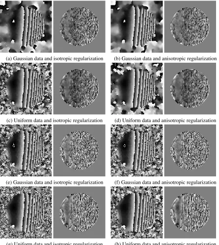
2.9 Example low-pass filtering results using the Augmented Lagrangian solver (a to d) and the Proximal Bregman solver (e to h). Each pair includes the low-pass filtered image and a difference image between the result and the noise-free phantom image, Fig. 2.8b. . . 41
2.10 Error reduction with varying regularization weight . . . 42
2.11 Single channel cranial MR image including magnitude (a) and phase (b) com-ponents. . . 43
2.12 Local phase shift maps on the single channel MR image shown in Figure 2.11. . 45
2.13 Local Phase Shift Map computed via channel combination of single channel local phase shift maps such as those presented in Figure 2.12. . . 46
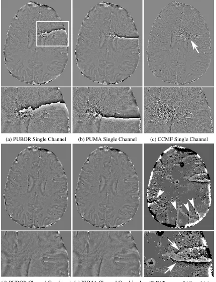
2.14 Residual phase wrapping artifacts present in channel combined images created
using phase unwrapping paradigm. . . 47
2.15 CNR performance over echo time . . . 48
2.16 Confidence intervals on mean CNR difference between methods . . . 48
3.1 Example of anatomical knowledge in the form ofpart/whole relationships ex-pressing the decomposition of the cerebral cortex into hemispheres and then into individual lobes. . . 52
3.2 Example label ordering from Figure 3.1 shown in diagrammatic form. . . 53
3.3 Potts and Ishikawa models in terms of label ordering . . . 55
3.4 Example of the different label ordering operators . . . 56
3.5 Label orderings used in cardiac segmentation by Rajchlet al.[149, 150] . . . . 57
3.6 Example of transforming a hierarchical label ordering into a flow network. . . . 60
3.7 Pipeline used in multi-atlas brain tissue segmentation. . . 65
3.8 Hierarchical label ordering used in segmentation of the OASIS database . . . . 66
3.9 Best and worst case results for the OASIS database (top row: best case T1w im-age, gold standard, JLF+HMF, worst case T1w image, gold standard, JLF+IM+HMF; bottom row: enlarged ROIs.) . . . 69
3.10 Hierarchical label ordering used in segmentation of the OASIS database . . . . 72
3.11 Best case results for the MRBrainS database (top row: best case T1w image, T1IR image, T2FLAIR image, gold standard, JLF+IM+HMF. bottom row: en-larged ROI.) . . . 74
3.12 Worst case results for the MRBrainS database (top row: best case T1w image, T1IR image, T2FLAIR image, gold standard, JLF+IM+HMF. bottom row: en-larged ROI.) . . . 74
4.1 Segmentation Interactivity Spectrum . . . 77
4.2 Example Sign Graphs in Segmentation Interfaces . . . 84
4.3 Segmentation interface with user seeds before segmentation (a) and after seg-mentation (b). The hierarchy definition widget (bottom left corner of (a) and (b) ) is shown enlarged in (c). . . 91
4.4 Cardiac segmentation with underlying (a) CT, (d) MRA, and (g) TEE. Manual segmentations are in (b), (e), and (h) respectively, and interactive segmentation results in (c), (f), and (i). . . 93
4.5 Neonatal Ventricle Segmentation with (a) the MR, (b) the manual segmenta-tion, and (c) interactive segmentation results. (d) shows surface renderings of both the fully manual (left) and interactive (right) segmentation results. . . 94
4.6 Pathological Neonatal Ventricle Segmentation with (a) the MR, (b) the man-ual segmentation, and (c) interactive segmentation results. (d) shows surface renderings of both the fully manual (left) and interactive (right) segmentation results. . . 95
4.7 Hierarchies used in (a) healthy and (b) pathological neonatal ventricle segmen-tation. . . 95
(d) manual segmentation and (e) interactive segmentations results. . . 96
5.1 Schematic vessel bifurcation . . . 102 5.2 Two possible hierarchical label orderings for the vessel bifurcation
segmenta-tion example shown in Figure 5.1. . . 102 5.3 DAG for segmentation into labels L = {A,B,C,D,E} in which label groups
G= {AB,BC,CD}are regularized. Note that this would be impossible in a
hi-erarchical model since the regularization groups conflict with each other. Fig-ure 5.3a shows the intermediate multi-edged, unweighted DAG. FigFig-ure 5.3b shows this DAG with weights explicitly recorded rather than through multi-plicity which is used by the solution algorithms. . . 106 5.4 Synthetic image (a) polluted with noise (b) and reconstructed using a Potts
model (c), DAGMF (d) and HMF models with either the red square (e) or green circle (f) regularized.Weighted DSC is given for each segmentation. . . . 111 5.5 Directed acyclic graph and weights used for DAGMF segmentation shown in
Figure 5.4. The nodescircleandsquare denote the labels associated with the union of green with yellow and red with yellow respectively. . . 112 5.6 DAG representing the brain tissue segmentation problem in Fig. 5.8. . . 112 5.7 Bayesian data terms used in Fig. 5.8. . . 113 5.8 Brain tissue segmentation using DAGMF using data terms in Fig. 5.7 and
constant smoothness terms. Note the improvement in the pink subcortical gray matter region. . . 114 5.9 Segmentation uncertainty (entropy) from Figure 5.8. The Potts model has much
higher uncertainty in the background segmentation around the frontal lobe. . . . 115 5.10 Segmentation structure used in scene decomposition into F-front, T-top,
B-bottom,L-left,R-right. The color code corresponds to that used in Figure 5.11. 116 5.11 Example outdoor scene segmentation. Accuracy rate is given for each
segmen-tation. The color code for the segmented images are shown in Figure 5.10. . . . 117 5.12 Example scene segmentation from the Stanford indoor dataset [42]. DTO refers
to the “data term only” method. Accuracy rates are given for each segmenta-tion. Label orderings used in the first and second HMF segmentation are shown in (f) and (i) respectively. The color code for the segmented images are shown in Figure 5.10 and in (f) and (i). . . 118 5.13 Example DAG for hue reconstruction withN = 9 discrete hues and a truncated
linear model of widthM= 3. Although not shown, the weight of each edge on the top level is 1, and 1/Mon the bottom layer. . . 120 5.14 Hue reconstruction on synthetic image with corresponding normalized hue error. 120 5.15 Example hue reconstruction on natural images with DAGMF model (N =
36,M =16). . . 121 6.1 Simple star convex objects with vantage points indicated with an ‘X’. . . 126
6.2 Synthetic image segmentation problem using DAGMF (2e) and DAGMF aug-mented with shape complexes (2f) according to the label ordering in (2d) with
αreferring to the level of regularization. (* a simple star convexity constraint is applied to this label.) Any overlap between segmentations can cause false colors, e.g. green occurs when the result is 50% exterior (cyan) and 50% in-terior (yellow). The ‘X’ marks the vantage point for the simple star convexity constraint. . . 134 6.3 Quantitative segmentation results for each region based on regularization strength.
The Dice similarity coefficients are shown on a logarithmic scale approaching 100% DSC. . . 135 6.4 Venn diagram segmentation with and without shape complexes. The label
or-dering is given in Figure 4c (* a simple star convexity constraint is applied to this label) with the vantage point for the shape complex was the centroid of the region. Similar to Figure 6.2, any overlap between segmentations can cause false colors. . . 136 6.5 Vessel segmentation in ultrasound with and without shape complexes. The
label ordering is given in Figure 5c (* a simple star convexity constraint is applied to this label) with the vantage point for the shape complex is marked with an ‘X’. Similar to Figure 6.2, any overlap between segmentations can cause false colors. . . 137 6.6 Quantitative results for the segmentation problem shown in Fig. 6.5 varying
regularization and bias parameters. Blue indicates DSC ≈ 0 and yellow indi-cates DSC≈ 1 as shown in Fig. 6g. . . 138 6.7 Synthetic valve annulus segmentation. The label K indicates the background
(in cyan),T W andBW indicates the top and bottom walls respectively (in ma-genta), T B and BB indicate the top and bottom blood pools respectively (in yellow), andV indicates the valve annulus (in green). . . 139 6.8 Mitral valve labelling using trans-esophageal ultrasound images. The model
(Figure 6.7a - previous figure) includes label K indicates the background (in cyan), T W and BW indicates the top and bottom walls respectively (in ma-genta), T B and BB indicate the top and bottom blood pools respectively (in yellow), andV indicates the valve annulus. . . 139 6.9 Atrial wall segmentation DAGMF augmented with shape complexes with α
representing the regularization strength. (* a simple star convexity constraint is applied to this label.) . . . 141 6.10 Best and worst case atrial wall segmentation results. The atrial blood pool
is shown in magenta and the atrial wall in cyan. The black regions are user-provided seed points for the atrial blood label. . . 142
1.1 Split-Merge solution algorithm for binary max-flow proposed by Pock and
Cham-bolle [32, 137] . . . 16
1.2 Augmented Lagrangian solution algorithm for binary max-flow proposed by Yuanet al.[192] . . . 17
1.3 Proximal Bregman solution algorithm for binary max-flow proposed by Baeet al. [13] . . . 18
2.1 Split-Merge solution algorithm proposed by Pock and Chambolle [32, 137] for convex image restoration problems . . . 25
2.2 Augmented Lagrangian solution algorithm proposed by Yuanet al. [193] for the continuous Potts model . . . 27
2.3 Proximal Bregman solution algorithm proposed by Baxter et al. [18] for the continuous Potts model . . . 27
2.4 Augmented Lagrangian solution algorithm proposed by Baeet al. [14] for the continuous Ishikawa model . . . 31
2.5 Proximal Bregman solution algorithm proposed by Baxter et al. [18] for the continuous Ishikawa model . . . 31
2.6 Augmented Lagrangian solution algorithm for the CCMF functional in terms of indicator functions. . . 37
2.7 Proximal Bregman solution algorithm for the CCMF functional in terms of in-dicator functions. . . 38
3.1 Augmented Lagrangian solution algorithm for the HMF functional. . . 61
3.2 Proximal Bregman solution algorithm for the HMF functional. . . 62
5.1 Augmented Lagrangian solution algorithm for the DAGMF functional. . . 108
5.2 InitializeSolution()subroutine in Algorithm 5.1. . . 108
5.3 UpdateFlows()subroutine in Algorithm 5.1. . . 109
5.4 Proximal Bregman solution algorithm for the DAGMF functional. . . 110
6.1 Augmented Lagrangian solution algorithm for Eq. (6.3). . . 130
6.2 InitializeSolution()subroutine in Algorithm 6.1. . . 131
6.3 UpdateFlows()subroutine in Algorithm 6.1. . . 132
6.4 Proximal Bregman algorithm for Eq. (6.3). . . 133
List of Tables
2.1 Computation times for 2D image slices at varying echo time . . . 44 2.2 Three-way ANOVA Table of factors affecting CNR . . . 48
3.1 Segmentation Results - OASIS: significantly better metrics (p ≤ 0.05 after Bonferroni correction) between HMF/Potts pairs are shown in bold and signif-icantly better metrics (p ≤ 0.05) with/without the intensity model are denoted with an asterix for JLF. . . 69 3.2 Comparison Results - OASIS DSC: significant difference to JLF+IM+HMF
(p≤0.05after Bonferroni correction) is shown in bold . . . 70 3.3 Comparison Results - OASIS AVD: significant difference to JLF+IM+HMF
(p≤0.05after Bonferroni correction) is shown in bold . . . 70 3.4 Comparison Results - OASIS MHD: significant difference to JLF+IM+HMF
(p≤0.05after Bonferroni correction) is shown in bold . . . 70 3.5 Segmentation Results - MRBrainS: significant difference to JLF+IM+HMF
(p≤0.05after Bonferroni correction) is shown in bold . . . 73 4.1 Classification with examples of different input sign types . . . 80 4.2 Examples of different output sign types . . . 82 4.3 Cardiac Segmentation Numerical Results. Results shown inboldindicate
met-rics that are common across SEGUE, manual segmentations, and [149] which can be used as a reference for comparison . . . 92 4.4 Scar Tissue Segmentation Results. Results shown inboldindicate metrics that
are common across SEGUE, manual segmentations, and [150] which can be used as a reference for comparison . . . 97
5.1 Dice coefficient for segmentations in Fig. 5.8. The results for the subcortical gray matter are shown inboldwhich reflect the quantitative improvement from using a more nuanced regularization model with DAGMF. . . 114 5.2 Value of the constant regularization terms used in the various max-flow models. 117 5.3 Accuracy rates for segmentations in the Stanford indoor dataset such as that
shown in Fig. 5.12. DTO refers to the “data term only” method. The results shown inboldrepresent those statistically significantly different from the DTO method under a paired t-test with Bonferroni correction. . . 118
6.1 Mean distance error results for the blood pool and whole atrium labels. These are reflective of the errors seen on the inner and outer boundary of the atrial wall label. . . 141
Appendix A Use of the Principle of Duality and Derivations of Algorithms . . . 153 Appendix B Combinatorial and Complexity Analysis of Label Ordering Structures . . . 180 Appendix C Ethics Approvals for Patient Images . . . 182 Appendix D Copyright Transfers and Reprint Permissions . . . 187
List of Abbreviations, Symbols, and Nomenclature
Mathematical and Computer Graphics/Vision Terminology
A−> Inverse transpose of a square matrix (i.e. A−> =(A−1)>=(A>)−1) 2S The power set ofS, or set of all subsets ofS
2D Two dimensional
3D Three dimensional
Ω Spatial domain
ANR Artefact-to-noise ratio
CNR Contrast-to-noise ratio
DAG Directed Acyclic Graph
GPGPU General-Purpose Graphics Processing Unit
GPU Graphics Processing Unit
MAP MaximumA PosterioriProbability
MRF Markov Random Field
ND ArbitraryNdimensional
NP Non-Deterministic Polynomial
NPC Non-Deterministic Polynomial Complete
PGM Probabilistic Graphical Model
Medical Imaging Terminology
CT Computed Tomography
CTA Computed Tomographic Angiography
MR Magnetic Resonance
MRI Magnetic Resonance Imaging
QSM Quantitative Susceptibility Mapping
ROI Region of Interest
STI Susceptibility Tensor Imaging
SWI Susceptibility Weighted Imaging
T1 Longitudinal Relaxation Time
T1IR T1 Inversion Recovery
T2 Transverse Relaxation Time
T2FLAIR T2 Fluid Attenuated Inversion Recovery
US Ultrasound
Terms Introduced by this Thesis
I Image Intensity Range
L Set of labels forming a partition in a segmentation problem G Set of superlabels requiring separate regularization
CCMF Cyclic Continuous Max-Flow
DAGMF Directed Acyclic Graphical Continuous Max-Flow
HMF Hierarchical Continuous Max-Flow
To the reader, this thesis focuses on a relatively recent technical and theoretical development in image processing: continuous max-flow. Continuous max-flow theory is a continuous ana-logue to graph-cut theory which has received wide attention from computer scientists since the 1950s and computer vision scientists since the 2000s. The continuous max-flow commu-nity however grew out of the convergence of many different mathematical theories, notably graph-cuts, variational optimization and level set optimization, all of which tended towards conflicting notation.
I have attempted to reconcile the notation used by the many authors in the continuous max-flow community, to express discrete graph-cuts in an analogous notation, and to enforce some notion of stylistic integrity. If I do not use the reader’s preferred notation in any particular section, I apologize. My goal is only to emphasize the growth of the field and the many similarities contained within.
On a related note, the literature contains many a phrase like “Optimize f(x) which can be done analytically”and leaves it at that. Wherever possible, I have replaced this with the an-alytic solution. I present pseudocode for many algorithms in a style that I hope is readily understandable and implementable. Once again, the goal is clarity and completeness, not ob-fuscation. To make this possible, one must assume a certain degree of background knowledge of the reader, such as the standard notation in formal logic and set theory.
I hope you find this thesis to be informative and hopefully entertaining.
Regards,
John S.H. Baxter
Chapter 1
Introduction
1.1
Images and Image Labelling Problems
What is an image? To begin on a formal note, an image is anintensity function, I(x) : Ω → I, which maps a spatial location x ∈ Ω, to an intensity i ∈ I, often a real vector of pre-defined dimensionality (i.e. I = Rn). How one understands or models this intensity function and its underlying spatial domainΩhas a large effect on what form image analysis problems can take. Changing howΩ is interpreted changes what mathematical formalisms can be expressed. For example, one could consider a photograph ornatural image to be a functional of a finite 2D lattice of pixels (that is, Ωis a finite set). Because the domain Ω is a discrete lattice, the traditional concept of derivatives and curvature do not exist, requiring infinitesimally small but non-zero distances. (Approximations or analogues such ascalculus of finite differencesexist and somewhat bridge the gap in formalisms, but still illustrate that differences in the topology of the spatial domain have an effect on how the labelling problem is formulated.) If instead the natural image is interpreted as having a 2D continuum domain Ω, rather than a lattice, these traditional notions based on infinitesimally small distances are restored, encouraging us to use a different collection of theoretical tools to address labelling problems using this image as input.
This thesis will concentrate on low-level labelling (or just labelling) problems. These are image analysis problems that can be expressed in the form of alabelling function,u(x), which maps spatial locations on the image,x∈Ω, to one of:
• an element of a predefined finite set of values (i.e. image partitioning), • a subset of a predefined finite set of values (i.e. image segmentation),
• a continuous interval of values (i.e. image enhancement, restoration, filtering, etc...), or • a location in another spatial domain (i.e. image registration).
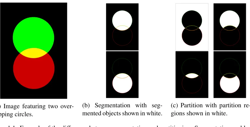
(a) Image featuring two over-lapping circles.
(b) Segmentation with seg-mented objects shown in white.
(c) Partition with partition re-gions shown in white.
Figure 1.1: Example of the difference between segmentation and partitioning. Segmentation problems may, in general, involve regions that overlap or may not cover the image. Partitioning problems require non-overlapping regions which altogether cover the entire image.
1.1.1
Partitioning and Segmentation Problems
The reader may confused over why there is a difference between a partitioning problem and a segmentation problem. In fact, a partitioning problem can be expressed as a subset of seg-mentation problems in which the subsets mapped to always contain only one element. In some segmentation problems, this may not be the case, especially if objects overlap or if one object is described as spatially containing another such as a vessel containing a lumen. Although this distinction may appear pedantic, it will become important later on.
Figure 1.1 shows an example of the difference between segmentation and partitioning prob-lems. The key difference is that segmentation problems are more general; they do not require the regions being segmented to be disjoint or to cover the entire image. Partitions on the other hand, must cover the entire image and cannot be overlapping.
Often, the labelling function will be described in terms of an indicator function. In those cases, the indicator function corresponding to a particular label,L, will be written asuL(x). In a segmentation or partitioning problem, these indicator functions can be defined as:
uL(x)=
1, ifx∈L
0, else (1.1)
which have the property that if a subset ofL’s,L, forms a partition:
X
∀L∈L
1.1. Images andImageLabellingProblems 3
Fuzzy indicator functions are a less constrained type of indicator function that take on a value in the interval [0,1] with higher values being indicative of membership in the corresponding label. Fuzzy indicator functions have the same partitioning property described in Equation 1.2. The subscript notation on the indicator functions was intended to be similar to that commonly used for indexing vector valued functions, although in this case, the indices are not integers but labels.
Partitioning problems are obviously a constrained class of segmentation problem. However, any segmentation problem can be converted into a partitioning problem by considering the power set 2L. This is an important technique as many of the elements of 2Lmay not be feasible and their indicator function is constrained to equal 0.
1.1.2
Image Enhancement, Restoration and Filtering Problems
Image enhancement, restoration and filtering problems involve assigning locations with a new intensity function. Often, image restoration and enhancement problems use the same inten-sity function range as the original image. A useful representation of these problems involves approximating them with a partitioning or segmentation problem once. That is, the labelling function (i.e. the processed image),u(x), can piecewise-constant approximated as:
u(x)≈ N X
i=1 ˜
uiui(x) (1.3)
where ˜uiis an intensity andui(x) is an indicator function for the partitioning problem expressing that location x has a processed intensity of approximately ui. That is, ui(x) = 1 if and only if u(x) ≈ ui. (If fuzzy indicator functions are used, this becomes a linear approximation.) This approximation can become arbitrarily good given a larger and larger number of indicator functions with closer and closer values ofui. An important result of this is that a function of a location and its label value can also be approximated:
f(u(x),x)≈ N X
i=1
f(ui,x)ui(x) (1.4)
1.1.3
Image Registration Problems
Image registration involves associating every spatial location in an image to a spatial location in another image or atlas. In the case ofrigidandaffineregistration problems, this mapping has a very particular form and thus can be represented more readily as a constant transform. In that case, it is rare to see it represented as an image labelling problem. Deformable registration, on the other hand, is often represented as a labelling through the use of a deformation field. That is, the spatial location being mapped to is equal to the original spatial location with some translational offset, ory= x+d(x) wherey,x∈Ω[179].
Maintz and Viergever [116, 179] provided a popular taxonomy for medical image registra-tion techniques composed of the interrelated criteria:
1. Dimensionality of the image(s) involved, 2. Modalities of the images(s) involved,
3. Subjects involved (intra-subject, inter-subject, atlas), 4. Objects-of-interest involved,
5. Degree of interaction (interactive, semi-automatic, automatic),
6. Nature of the registration basis (extrinsic fiducials, intrinsic landmarks, segmentation-based, image-segmentation-based, calibrated co-ordinate system based),
7. Nature of the transformation (rigid, affine, projective, spline-interpolated, fully deformable), 8. Domain of the transformation (local or global), and
9. Optimization procedure involved in determining said transformation.
The first four criteria roughly align to clinical context of the registration problem, the next five to what constraints are placed on the labelling, and the last pertains to how such a labelling is determined. A comprehensive review of medical image registration approaches is beyond the scope of this thesis, but the interested reader can consult the recent review article by Viergever et al. [179] or the review article specifically concerning deformable registration by Sotiraset al. [164].
1.2
Markov Random Fields and Gibbs Distributions
One invaluable theoretical tool for labelling problems in general is theMarkov Random Field (MRF). An MRF is an undirected probabilistic graphical model, that is, a probability distribu-tion concerning the values of a collecdistribu-tion of variables represented as nodes in a graph,G. The edges in a graph define the threeMarkov properties[101]:
1.2. MarkovRandomFields andGibbsDistributions 5
2. Local Markov Property: The value of any variable (v∈G) is conditionally independent of all other variables given its neighbours.
3. Global Markov Property: The values of any two disjoint sets of variables (V,W ∈ 2G) are conditionally independent given a third separating set.
These properties increase in strength, that is, the global Markov property implies the local, which in turn implies the pairwise. In image labelling problems, the goal of using an MRF is to express more desirable labelling configurations as being more probable.
The probability distribution expressed by a MRF must be aGibbs distribution. Specifically, the probability distribution can be expressed in the form:
P(u)= e
−E(u)
Z (1.5)
where E(u) is an energy function andZ is a normalization factor. The energy function maps the state configuration to a real number, with higher numbers representing less probable con-figurations. Representing an MRF via a Gibbs distribution is important because many MRF’s of interest can be specified using a particular constrained set of energy functions, specifically those which can be decomposed as:
E(u)= X
∀V∈cl(G)
E(uV) (1.6)
where thecliqueoperator, cl(·), is the set of all sets of variables inGsuch that every variable is adjacent to every other variable. More formally:
cl(G)=nV ∈2G| ∀(v,w)∈V,w= vorw∈ NG(v) o
(1.7)
This is called theclique factorizationof the MRF. Terms in which V has one or two variables are calledunaryandbinaryenergies respectively. One particularly important result along these lines is theHammersly-Clifford theorem[68] which states that the MRF has a strictly positive probability for every configuration if and only if it can be expressed via a clique factorization.
1.2.1
Unary and Binary Energies
Unary energies (often called data terms) are important in labelling problems because they directly relate the labelling value at a particular location to local properties such as the spatial location or image intensity. One particularly useful form of data term used in segmentation is theBayesiandata term, which can be written as:
DL(x)=−ln (I(x)|x∈L)+lnP(x∈L). (1.8)
This type of data term uses the probability distribution encoded in the MRF directly, that is, it defines the probability of a particular region taking on a particular label in the absence of neighbours to affect it. In image enhancement problems, a common data term is the difference between the intensity and the labelling taken to some power:
D(u(x),x)= |u(x)−I(x)|p. (1.9)
Being based on a single voxel, data terms can be sensitive to noise in the image.
Binary energies (often called first-order terms or regularization terms) control how much adjacent variables effect each other. The reason these are called regularization terms is that they are used to smooth away any overfitting caused by the data terms. A common regularization term in partitioning problems is the uniform term:
R(x,y)=
0, ifu(x)= u(y)
α, else (1.10)
whereαis a positive constant. Other common regularization terms replace the constantαwith a positive monotonically decreasing function of the difference in intensity between the two locations:
R(x,y)=
0, ifu(x)=u(y)
f(|I(x)−I(y)|), else . (1.11)
These terms penalizes variation in the labelling less if it is associated with variation in the image intensity, thus encouraging edges in the labelling to align to edges in the image.
1.3. DiscreteGraph-Cuts 7
1.3
Discrete Graph-Cuts
For MRFs with zero higher order clique energies and non-negative regularization terms taking the form specified in the previous section, graph-cut approaches have been favored due to their speed and optimality guarantees. This is largely because the MRF can be expressed as an edge-weighted graph in which a binary labelling (u(x)∈ {0,1}) is related to a cut through this graph where a cut is a minimal set of edges that, if removed, disconnect the source and sink nodes. The MAP optimum (i.e. energy minimum) is thus related to the minimum weighted cut.
1.3.1
Discrete Ising Model
The Ising model [79] is arguably the simplest MRF, in which each variable can only take on a single value, either a 0 or a 1, and was designed to model polarization in ferromagnetic materials. This model has great implications to image segmentation in that it can be seen as it could be seen as a representation of a binary segmentation problem, one with a single object-of-interest and the background. The equation for this model is:
E(u)=X x∈Ω
D(x)u(x)+X x∈Ω
X
y∈N(x)
R(x,y)
2 |u(x)−u(y)| (1.12)
which contains a data term, P
x∈ΩD(x)u(x), and regularization term, Px∈ΩPy∈N(x) R(x,y)
2 |u(x)− u(y)|. (See Section 1.2.1.)
Greig et al. [64] were the first to use max-flow to address an MRF in image processing, specifically the Ising model. The Ising model can be easily recrafted in a graphical representa-tion given the smoothness term is non-negative and symmetric. In this graph, there is a ‘spatial’ vertex for each voxel in the image which are adjacent to a source vertex, s, and a sink vertex, t. The weight of the edges between spatial vertices would be the smoothness term, the weight between spatial vertices andsbeing max{0,D(x)}, and the weight between spatial vertices and t being max{0,−D(x)}. In this form, the MAP labelling can be expressed as the graph-cut problem:
argmin u(x)
X
x∈Ω
max{0,D(x)}u(x)+X x∈Ω
max{0,−D(x)}(1−u(x))+X x∈Ω
X
y∈N(x)
R(x,y)
2 |u(x)−u(y)| (1.13)
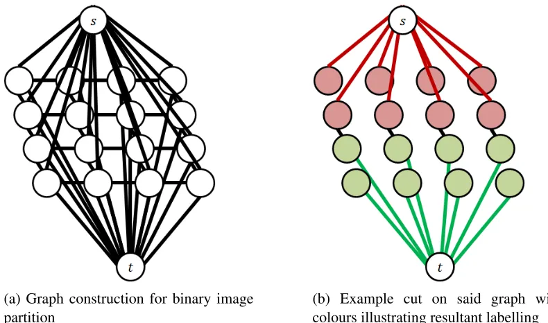
(a) Graph construction for binary image partition
(b) Example cut on said graph with colours illustrating resultant labelling
Figure 1.2: Example of a 4-connected graph construction and cut representing a binary image partition problem.
edge, that edge is part of the minimum cut, that is, the edges that, when removed, partition the graph into two sub-graphs, one with s and the other witht, such that the weight of the edges removed is minimized. Techniques for handling this max-flow/min-cut problem include:
• Augmenting paths algorithms based on the original algorithm by Ford and Fulkerson [57], where paths with excess capacity are identified and saturated; and
• Push-relabel algorithms [61], which order vertices by ‘height’ expressing their capacity to accept additional incoming flow.
In binaryND image segmentation problems, the most common neighbourhood configura-tion used is the rectilinear lattice. In this lattice, each variable (i.e. pixel/voxel) is connected to 2× N others, one pointing upwards and another downwards in each of the N orthogonal directions [24, 26]. An example of said graph is given in Figure 1.2a. A cut through said graph must associate each node with either the source or sink vertex, thus partitioning the image as shown in Figure 1.2b. The remaining edges in the cut represent the boundary of the object.
1.3.2
Applications of Graph-Cuts in Medical Image Processing
1.4. ContinuousMax-FlowTheory 9
• segmentation of a single object of interest [23, 27] including the prostate [114, 200], liver [166], lungs [4, 29], kidneys [5, 154], cardiac ventricles [11, 84, 104, 115], the whole brain [112, 155] and various neurological structures such as the hippocampus [176], • segmentation of multiple objects of interest [43, 44] including the abdominal cavity
[126],
• MRI phase unwrapping [22, 188], • fat-water separation in MRI [71],
• medical image fusion for visualization [121], and • deformable image registration [110, 163, 170].
1.4
Continuous Max-Flow Theory
This section explores the max-flow equation:
E(u)= Z
Ω
D(x)u(x)dx+ Z
Ω
R(x)|∇u(x)|dx s.t.u(x)∈ {0,1}
(1.14)
its relationship to the MRFs examined in the previous section, and previous work in minimizing this equation. This equation is the analogue to the Ising model in equation 1.12 in that contains contains a data term, RΩD(x)u(x)dx, and regularization term, RΩR(x)|∇u(x)|dx which fulfil the same practical roles as they do in the discrete model. (See Section 1.2.1.) The labelling function, similarly, takes on a value of either 0 or 1.
Before exploring continuous max-flow, the notions of convexity and convex relaxation should be introduced. Convexity is a property of both sets and of real-valued functions. A set is convex if and only if, for any two elements in the set, any point on the line segment connecting those elements is also in the set. Formally, a set, C is convex if and only if ∀(c1,c2)∈C,∀λ∈[0,1](λc1+(1−λ)c2 ∈C). A function is convex if and only if the epigraph (the set{(x,y)|y≥ f(x)}) is a convex set. This is equivalent to the definition that:
f(x) is convex if and only if
∀(x1,x2)∈Ω,∀λ∈[0,1] (λf(x1)+(1−λ)f(x2)≥ f(λx1+(1−λ)x2)).
(1.15)
to first apply convex relaxation to the indicator function constraint u(x) ∈ {0,1}which yields the constraints thatu(x) ∈ [0,1] and thatu(x) must have bounded variation, that is, it must be approximately smooth. In the context of segmentation, convex relaxation transforms a standard segmentation problem into a fuzzy segmentation problem that is easier to solve.
1.4.1
From Discrete Graph-Cuts to Continuous Max-Flow
As a thought-experiment, consider taking a space and sampling it with a rectilinear lattice as described by Boykovet al.[24, 26]. The spacing between points on the lattice will be denoted ∆r. A continuum model can be developed by letting∆r → 0, that is, by making a denser and denser lattice, as shown in Figure 1.3. Before doing this, one must specify how the data terms and regularization terms change as this lattice gets denser. In particular, one must develop effective data and smoothness terms ˜D(x) and ˜R(x,y) with desirable limiting case properties, including:
• Both ˜D(x) and ˜R(x,y) grow proportional to the volume element, for the rectilinear sam-pling case of a D-dimensional space with an isotropic inter-sampling distance of ∆r, ∆V = (∆r)D. This intuitively means that as the graph is sampled more, each individual node and edge has a lower and lower importance, there being more of them.
• R(x˜ ,y) is proportional to an underlying smoothness fieldRx+2ywhich is differentiable, i.e.∇R(x) is finite. ˜D(x) should also be proportional to some underlying function D(x).
• R(x˜ ,y) grows inversely proportional to the spacing in between neighbours, that is|x−y|. That is, as the spacing gets smaller, knowing the label of an adjacent variable has more value.
Fulfilling these properties yield the terms ˜D(x) = D(x)(∆r)D and ˜R(x,y) = R( x+y
2 )(∆r)
D
|x−y| . For
now, assume thatN(x) contains only the variables immediately adjacent to xin each of theD
1.4. ContinuousMax-FlowTheory 11
directions. Using these assumptions, one can take the limiting case of the energy equation:
E(u)= lim ∆r→0
X
x∈Ω
˜
D(x)u(x)+X x∈Ω
X
y∈N(x) ˜ R(x,y)
2 |u(x)−u(y)| = lim ∆r→0
X
x∈Ω
D(x)(∆r)Du(x)+X x∈Ω
X
y∈N(x)
R(x+2y)(∆r)D
2|x−y| |u(x)−u(y)| = Z
ΩD(x)u(x)dx+ Z
Ω X
y∈N(x) R(x) 2
∇u(x)· x−y |x−y|
dx = Z
ΩD(x)u(x)dx+ Z Ω R(x) 2 D X
i=1
|∇u(x)·ei|dx+ Z Ω R(x) 2 D X
i=1
|∇u(x)· −ei|dx E(u)= Z Ω D(x)u(x)dx+ Z Ω R(x) D X
i=1 δu(x)
δxi dx (1.16)
where ei is the unit vector along the ith axis. This formula implies that the regularization is applied to the L1 norm of the gradient magnitude. This L1 norm arises through the rectilinear nature of the lattice. This may not be appropriate in that it is not rotation invariant, like the L2 norm, and can lead to metrication artefacts.
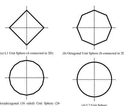
From a geometric sense, the neighbourhood function, N(x), has a quite distinct effect, especially in terms of the concept of norms. On a global level, the immediate adjacent neigh-bourhood, that is, the 4-connected (in 2D) or 6-connected (in 3D) is associated with the L1 norm. As the neighbourhood gets more connected, the associated norm can be thought of as a polygonal norm, that is, a norm in which the unit sphere appears to be a regular polygon. These norms, a selection of which are shown in Figure 1.4, approach the L2 norm as the neighbour-hood size increases.
Thus, an additional limit is needed. Not only should ∆r → 0, but also that the number of neighbours should approach infinity as shown in Figure 1.5, constructinginfinitely dense, infinitely densely connectedlattices. The last assumption is therefore:
• R(x˜ ,y) grows proportional to a surface area density (∆a) of the neighbourhood around x. Intuitively, this means that as a neighbourhood is more densely connected, knowing the labelling value of only one neighbour has less of an effect. The surface area density is assumed to converge to the L2 unit sphere, specifically having the property that, for any vectorθ∈ BD, as the size of the neighbourhood gets arbitrarily large,P
y∈N(x)∆ a|(x−y)·θ|
|x−y| →
(a) L1 Unit Sphere (4-connected in 2D) (b) Octagonal Unit Sphere (8-connected in 2D)
(c) Hexadecagonal (16 sided) Unit Sphere
(24-connected in 2D) (d) L2 Unit Sphere
Figure 1.4: Unit Spheres Under Various Norms
1.4. ContinuousMax-FlowTheory 13
found analytically using an inscribed regular polygon, specifically:
∆a=
2 sin(πn), wherexhas a clear path toy
0, else (1.17)
wherenis the number of said paths in the first case where x has a clear path toy with-out intersecting any other element in the neighbourhood. (Note that as N(x) gets an arbitrarily large number of elements, n also approaches infinity.) This approximation converges quickly, in that for as small asn= 8 (as in Figure 1.4b), the best possible in a square neighbourhood of radius 1,P
y∈N(x) ∆ a|(x−y)·θ|
|x−y| is in the interval [1.84,2]. Extending
the neighbourhood to have radius 2, that isn = 16 (as in Figure 1.4c), P
y∈N(x) ∆ a|(x−y)·θ|
|x−y|
is in the interval [1.96,2]. In 3D and higher dimensions, determining this surface area element can be more difficult as the neighbourhood size grows. However, for finite di-mensionality, it is always possible.
This constraint yields the terms ˜D(x) = D(x)(∆r)Dand ˜R(x,y)= R(x+2y)(∆r)D∆a
|x−y| . Using these four
assumptions, one can take the limit of the energy equation:
E(u)= lim ∆r→0nlim→∞
X
x∈Ω
˜
D(x)u(x)+X x∈Ω
X
y∈N(x) ˜ R(x,y)
2 |u(x)−u(y)| = lim ∆r→0nlim→∞
X
x∈Ω
D(x)(∆r)Du(x)+X x∈Ω
X
y∈N(x)
R(x+2y)(∆r)D∆ a
2|x−y| |u(x)−u(y)| = lim n→∞ Z
ΩD(x)u(x)dx+ Z
Ω X
y∈N(x)
R(x)∆a 2
∇u(x)· x−y |x−y|
dx = lim n→∞ Z
ΩD(x)u(x)dx+ Z
ΩR(x)
|∇u(x)| X y∈N(x)
∆a 2 ∇u(x) |∇u(x)|·
x−y |x−y|
dx E(u)= Z
ΩD(x)u(x)dx+ Z
ΩR(x)
|∇u(x)|dx
(1.18)
1.4.2
Duality and Convex Variational Optimization
Efficiently minimizing the max-flow energy, Eq (1.14), involves a branch of mathematics known of calculus of variations. This is a branch of mathematical optimization in which one tries to optimize a functional with an infinite number of degrees of freedom, rather than a function with a finite number. Because the energy, E(u) takes a functionu(x) as its argument, minimizing E(u) involves an infinite number of degrees of freedom, as there are an infinite number of spatial locations,xfor whichu(x) could take on a different value [51]. An important feature ofE(u) is its convexity; it satisfies the definition given in Eq (1.15).
The concept of dualityis an especially powerful tool in the analysis and optimization of convex functionals. In optimization theory, duality implies that any optimization problem can be viewed from two perspectives, a maximization and a minimization perspective, both of which form a bound on the value of the other. The duality gaprefers to the difference in the maximum value of the maximization problem and the minimum value of the minimization problem, which in the case of convex optimization problems is guaranteed to be 0. Throughout this thesis, three versions of the max-flow problem will be explored:
1. theprimalproblem of maximizing flow,
2. thedualproblem of minimizing energy, and
3. theprimal-dualproblem of doing both simultaneously.
These problems are formulated through the use of Lagrangian multipliers. That is, given a primal problem:
max x f(x)
such thatgi(x)= 0, i= 1,2, ...n
(1.19)
can be transformed into a primal-dual problem:
min
u maxx f(x)+ n X
i=1
uigi(x) (1.20)
where ui are the Lagrangian multipliers. From this, one can theoretically construct the dual functionof f(x) which is a function f0(u) with the definition:
f0(u)=max x
f(x)+
n X
i=1
uigi(x)
1.4. ContinuousMax-FlowTheory 15
which yields the third equivalent problem, the dual problem:
min u f
0
(u). (1.22)
The reader may notice that I used the same variable nameuto refer both to the dual variables and to the labelling function. This is because they are the same thing. Dual optimization is such a powerful tool for addressing functionals like Eq 1.14 because it allows for a flow maxi-mization problem through a particular network of continua to be used as the basic optimaxi-mization problem, and the minimum energy labellingis a result of the computational of the Lagrangian multipliers on various constraints in the network. That f0(u) is the same functional as E(u), with the exception that it takes on an infinite value wheneveru(x) is not a feasible labelling.
1.4.3
Early Approaches to Max-Flow Optimization
The first person to study max-flow optimization in the continuous domain was Gilbert Strang [167] who formalized the analogy between the discrete and continuous cases, providing the intuitive geometrical interpretation of the duality between maximizingRΩdivq(x)dxunder the constraint|q(x)| ≤1 and minimizingRΩ|∇u(x)|dx. However, it wasn’t until Antonin Chambolle [31] who developed the Chambolle iteration (now an essential component of current max-flow solution algorithms) that a truly primal-dual approach was developed. (Previous approaches involved estimating the solution of partial differential equations [7, 8, 33].) Chambolle’s ap-proach looked at a particular image restoration problem:
E(u)= Z
Ω
|I(x)−u(x)|2
2λ dx+
Z
Ω
|∇u(x)|dx. (1.23)
Chambolle used the primal function RΩdivq(x)dx under the constraint |q(x)| ≤ 1 to find the dual functionRΩ|∇u(x)|dx. From this, a projected gradient descent operator can be derived:
q(x)←Proj|q(x)|≤1
q(x)+τ∇(divq(x)−I(x)/λ) (1.24)
which is repeated untilq(x) converges, guaranteed ifτ≤1/8. The final step in this process is to calculateu(x) simply byu(x)= I(x)−λdivq(x)
The success of this image restoration algorithm led immediately to Pock and Chambolle developing a general max-flow solver using asplit-mergeapproach [32, 137]. In this approach, the max-flow functional is estimated by another functional of the form:
E(u,v)= Z Ω D(x)u(x)dx+ Z Ω
in which two similar solutionsu(x) andv(x) are iterated using gradient descent. The additional quadratic term in the middle encouragesu(x) andv(x) to approximate each other (or becoming equivalent as c → 0). If u(x) is fixed, the optimization problem becomes equivalent to the previous image restoration problem, and a series of Chambolle iterations can be used. Ifv(x) is fixed, the optimal value ofu(x) can be found analytically. The split-merge approach, shown in Algorithm 1.1, is to switch between fixing these two variables, both eventually converging.
Algorithm 1.1: Split-Merge solution algorithm for binary max-flow proposed by Pock
and Chambolle [32, 137]
whilenot convergeddo
whilenot convergeddo
q(x)←Proj|q(x)|≤1
q(x)+τ∇(divq(x)−u(x)/c);
end
v(x)←u(x)−cdivq(x);
u(x)←max{0, min{1, v(x)+cD(x)} };
end
1.4.4
Augmented Lagrangian Multipliers
Yuanet al. [192] took a similar approach, but provided a more computationally efficientfully primal-dual framework. In this framework, the primal model is taken to be the same max-flow problem suggested by Strang [167], that is:
max pS,pT,q
Z
ΩpS(x)dx (1.26)
subject to theflow conservation constraint:
G(x)=divq(x)+ pT(x)−pS(x)=0 (1.27)
and thecapacity constraints:
pT(x)≤max{0,D(x)} pS(x)≤max{0,−D(x)}
|q(x)| ≤R(x).
1.4. ContinuousMax-FlowTheory 17
Using the flow conservation constraint, the primal-dual model can be written as:
min u pmaxS,pT,q
Z
ΩpS(x)dx+ Z
Ωu(x)G(x)dx s.t. pT(x)≤max 0,D(x)
pS(x)≤max 0,−D(x) |q(x)| ≤R(x).
(1.29)
which can be shown to be equivalent to the dual problem of minimizing Eq (1.14).
Yuanet al.[192] perform the optimization on the primal-dual model with one small change; if an additional penalty term−R
Ω c 2G
2(x)dxwith positive constantcis applied to the equation, the maximization of pS(x) and pT(x) given all other variables can be determined analytically. This additional penalty is called an augmentation and the entire formula is called the aug-mented Lagrangian. Because it is independent of u(x), it does not effect the minimization component of the primal-dual model, and because it takes on its maximum value (of 0) only atG(x) = 0, it does not affect the optimal solution space of the maximization component of the primal-dual model. The only effect the augmentation has is the improved convergence rate [20]. The result is the optimization algorithm shown in Algorithm 1.2.
From this primal-dual view of the entire max-flow problem, Yuanet al. [192] were able to show that the global optimum to the max-flow functional under integrality constraintsu(x) ∈ {0,1}can be found by rounding the solution given by Algorithm 1.2 at a predefined threshold. This theorem is important for formal reasons, especially in partitioning problems, because it implies that global optimality can be guaranteed for both strict and fuzzy partitions.
Algorithm 1.2:Augmented Lagrangian solution algorithm for binary max-flow proposed
by Yuanet al.[192]
whilenot convergeddo
q(x)←Proj|q(x)|≤R(x)(q(x)+τ∇(divq(x)+ pT(x)− pS(x)−u(x)/c)); pT(x)←min{max{0,D(x)}, pS(x)−divq(x)+u(x)/c};
pS(x)←min{max{0,−D(x)}, pT(x)+divq(x)−u(x)/c}; u(x)←u(x)−c(divq−pS(x)+ pT(x));
end
1.4.5
Proximal Bregman Projections
terms of variational optimization, the precise technique used is theproximal Bregman projec-tion[28]. These projections are developed in a specific way. In order to optimize a function f(x), one can take a suboptimal solution x0 and improve it by finding a near-by solution with better value. Formally, each proximal Bregman projection can be written as:
x←argmin x
f(x)+cdg(x,x0)
(1.30)
where c is a positive constant and dg(·,·) is aBregman distance constructed out of a convex functiong(·). Specifically, this Bregman distance must have the formdg(x,x0)= g(x)−g(x0)−
δg·(x−y). [28] Baeet al.uses the entropy function:
g(u(x))= Z
Ω
(u(x) lnu(x)+(1−u(x)) ln(1−u(x)))dx (1.31)
which yields the Bregman distance
dg(u(x),v(x))= Z
Ω
u(x) ln(u(x)/v(x))+(1−u(x)) ln(1−u(x)/1−v(x))dx. (1.32)
The benefit of this Bregman distance is that it provides an infinite penalty on any solutionu(x) which violates the constraint u(x) ∈ (0,1). Similar to the algorithm proposed by Yuan et al. [192], the function being optimized is derived from the primal-dual model (which happens to have an analytic solution) and a Chambolle iteration is used to maximize the spatial flows. Unlike Yuan et al.’s approach however, Bae et al.’s formulation allows for the source and sink flow terms pS(x) and pT(x) respectively to cancel out of the optimization. The resulting algorithm is given in Algorithm 1.3.
Because the source and sink flows are implicitly represented rather than explicitly opti-mized, Baeet al.dub this thepseudo-flowapproach. In addition, the cancellation of the source and sink flows implies that less memory is required to use this algorithm.
Algorithm 1.3:Proximal Bregman solution algorithm for binary max-flow proposed by
Baeet al. [13]
whilenot convergeddo
q(x)←Proj|q(x)|≤R(x)
q(x)+τ∇exp−D(x)+divc q(x); u(x)← u(x) exp
−D(x)+cdivq
1−u(x)+u(x) exp−D(x)+divq
c ;
1.5. ContrastingGraph-Cuts andContinuousMax-Flow 19
1.4.6
Applications of Continuous Max-Flow in Medical Image Processing
Similar to graph-cuts, max-flow has received a significant amount of attention for a variety of medical image processing tasks. Often, these tasks are similar to those mentioned in Section 1.3.2. Recent applications of continuous max-flow include but are not limited to:
• Segmentation of a single object of interest including the prostate [143, 196], liver [135], cardiac ventricles [124, 148], cerebral ventricles [141], vasculature [175], and spine [12],
• Segmentation of multiple objects of interest including the prostate [142], brain [145] and lungs [66],
• Medical image fusion for visualization [195, 197], and
• Deformable registration, particularly for prostate [169] and cranial [146] MRI.
1.5
Contrasting Graph-Cuts and Continuous Max-Flow
The goal of this introduction was to show the smooth evolution of graph-cut, specifically the Ising model, into the corresponding continuous max-flow analogues. Thus, it has focused primarily on the conceptual equivalences and practical similarities between the two approaches. The goal of this section is to do the opposite, to focus on where the two methods diverge.
As illustrated in Section 1.4.1, in order to use graph cuts to approximate continuous max-flow, one must use not only an infinitely dense, but also an infinitely densely connected graph. This is infeasible in practice, resulting in a phenomenon known as a metrification artifact. These artifacts, an example of which is given in Figure 1.6, manifest as unwanted ’blockiness.’
(a) Original Image (b) Graph Cuts Segmentation (c) Max-Flow Segmentation
These metrification artifacts can also manifest as a preference for creating segmentation edges in a defined set of orientations, rather than at potentially arbitrary angles, as shown by Yuanet al [193]. These orientations are dependant on the connectivity of the neighbourhood used. For example, a 4-connected neighbourhood in 2D image segmentation results in a pref-erence for axis-aligned edges.
Another key difference between graph-cuts and max-flow is the computational complexity. The continuous max-flow algorithmic paradigms illustrated earlier (e.g. augmented Lagrangian and proximal Bregman projections) are iterative and numerical with computation time domi-nated by the convergence rate. Graph-cuts are know to have polynomial time algorithms for some configurations, while other configurations (such as the Potts model in Section 2.2.2) are known to be NP-hard meaning they can take a prohibitive amount of time to solve exactly. For these NP-hard problems, approximate solvers exist which also vary in their runtimes. Thus the computational complexity is much more varied across models for graph-cuts.
From a practical standpoint, the computation time difference between graph-cuts and max-flow depends heavily on the definition of the problem under investigation. For the 2D binary segmentation in Figure 1.6 which contains 256x256 pixels, the computation time for continu-ous max-flow with GPU acceleration was 0.4 seconds whereas graph-cuts using the Edmond-Karp algorithm [46] took 0.7 seconds, both implemented in MATLAB. Whether or not a par-ticular graph-cut or max-flow method is usable in practice heavily depends on the solution model being used. The additional benefit of the max-flow algorithms presented in this the-sis are that they are all trivially parallelizable, meaning that they can readily be implemented using GPGPU programming, unlike graph-cuts solvers based on the original Ford-Fulkerson algorithm [57].
1.6
Thesis Outline
This thesis will rely heavily upon the information presented in this introduction, especially that of Section 1.4 which is the theoretical and technical jumping-offpoint for the majority of the work presented.
The chapters are as follows:
• Chapter 2develops a cyclic continuous max-flow image enhancement model and apply it to processing phase information in MRI.
1.6. ThesisOutline 21
• Chapter 4motivates and develops an interactive segmentation interface that allows users to encode their own anatomical knowledge in an abstract form.
• Chapter 5 develops a continuous max-flow segmentation algorithm which can address all possible label orderings.
• Chapter 6develops a framework for encoding shape information into the previous con-tinuous max-flow segmentation algorithms, allowing for more complicated shapes to be specified.
Cyclic Continuous Max-Flow Image
Enhancement
This chapter is largely based on:
• John S.H. Baxter, Zahra Hosseini, Junmin Liu, Maria Drangova and Terry M. Peters. “Cyclic Continuous Max-Flow: Phase Processing Using the Inherent Topology of Phase.” Proceedings of ISMRM (2016).
• John S.H. Baxter, Zahra Hosseini, Terry M. Peters and Maria Drangova. “Cyclic Con-tinuous Max-Flow Phase Processing: A Third Paradigm in Generating Local Phase Shift Maps in MRI.” in revision for IEEE Transactions in Medical Imaging.
with additional material from:
• John SH Baxter, A. Jonathan McLeod, and Terry M. Peters. “A continuous max-flow approach to cyclic field reconstruction.” arXiv preprint arXiv:1511.03629 (2015).
2.1
Introduction
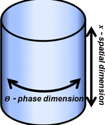
Image enhancement and restoration has long been a key problem in image processing literature. However, one aspect of image enhancement has fallen by the way-side, specifically therange topology, the topology equipped to the range (I) of the labelling function rather than its domain
(Ω) . Most images, such as photographs, have a Euclidean range topology and this topology is often implicitly assumed. However, some medical images, such as MR phase images, have a fundamentally different range topology.
Susceptibility-weighted imaging (SWI) and Quantitative Susceptibility Mapping (QSM) are types of MRI sensitive to tissue magnetic susceptibility which is encoded in the phase information encapsulated in the raw MRI data. Because slight changes in tissue magnetic