A Class of Solvable Optimal Stopping Problems of Spectrally Negative Jump Diffusions

(1)

L.H.R. Alvarez – T.A. Rakkolainen

A Class of Solvable Optimal

Stopping Problems of Spectrally

Negative Jump Diffusions

Aboa Centre for Economics

Discussion Paper No. 9

Turku 2006

(2)

Copyrigt © Author(s)

ISSN 1796-3133

Turun kauppakorkeakoulun monistamo

Turku 2006

(3)

Luis H. R. Alvarez

–

Teppo A. Rakkolainen

A Class of Solvable Optimal Stopping

Problems of Spectrally Negative Jump

Diffusions

Aboa Centre for Economics

Discussion Paper No. 9

October 2006

ABSTRACT

We consider the optimal stopping of a class of spectrally negative

jump diffusions. We state a set of conditions under which the

value is shown to have a representation in terms of an ordinary

nonlinear programming problem. We establish a connection

between the considered problem and a stopping problem of an

associated continuous diffusion process and demonstrate how this

connection may be applied for characterizing the stopping policy

and its value. We also establish a set of typically satisfied

conditions under which increased volatility as well as higher

jump-intensity decelerates rational exercise by increasing the value

and expanding the continuation region.

JEL Classification: C61, G11, G12

Keywords: jump diffusions, optimal stopping, nonlinear

programming, perpetual American options

(4)

Contact information

Luis H. R. Alvarez

Department of Economics

Turku School of Economics

FIN-20500 Turku

and

RUESG/Department of Economics

University of Helsinki

P.B. 17

FIN-00014 University of Helsinki

Teppo A. Rakkolainen

Department of Economics

Turku School of Economics

FIN-20500 Turku

Acknowledgements

The financial support from the

Foundation for the Promotion of the

Actuarial Profession

, the

Finnish Insurance Society

, and the

Research

Unit of Economic Structures and Growth (RUESG)

at the University

of Helsinki to Luis H. R. Alvarez is gratefully acknowledged.

(5)

1 Introduction

It is a well-known result from literature on mathematical finance that the price of a perpetual American option on an underlying asset whose value can be char-acterized as a stochastic process coincides with the value of an optimal stopping problem for this process (see, for example, Karatzas and Shreve (1999) pp. 54– 87 and Øksendal (2003), pp. 290–298). Such option prices, while naturally of interest in themselves, can also be used as upper bounds for prices of American options with finite expiration dates. Thus, their role is of importance from a risk management point of view as well. Perpetual optimal stopping problems arise quite naturally also in the real options literature on the valuation of irre-versible investment opportunities (see Dixit and Pindyck (1994) for an extensive textbook treatment of this theory). In that modeling framework the investment decision is usually interpreted as an opportunity (but not obligation) to obtain a stochastically fluctuating return in exchange from a payment (sunk cost) which may or may not be stochastic as well. Given the considerable planning horizon of the valuation of real investment opportunities, the time horizon is typically assumed to be infinite and, consequently, the considered optimal timing problem of the investment opportunity is assumed to be perpetual.

When the dynamics of the underlying process are characterizable via an Itˆo stochastic differential equation of form

dXt=µ(Xt)dt+σ(Xt)dWt (1)

withW a standard Wiener process, the stopping problem has been widely stud-ied by relying on various techniques. The probably most usually applstud-ied ap-proach is to rely on variational inequalities or the classical Hamilton-Jacobi-Bellman approach due to its applicability in a multidimensional setting as well (cf. Øksendal (2003) and Øksendal and Reikvam (1998)). In the one-dimensional setting there are, however, several different techniques for analyzing the perpetual stopping problem. The most general approach is probably pro-vided by studies relying on the integral characterization of excessive functions for diffusion processes and the Martin boundary theory (cf. Salminen (1985)

(6)

and Borodin and Salminen (2002), pp. 32–35). Alternatively, the considered problem can be analyzed by relying on the relationship between functional con-cavity andr-excessivity along the lines of the pioneering work by Dynkin (1965) (Chapters XV and XVI) and by Dynkin and Yuskevich (1969) which has been subsequently applied within a general optimal stopping framework in Dayanik and Karatzas (2003). A third technique for studying the perpetual optimal stopping in the linear diffusions setting is provided by the approaches relying on the well-known relationship between excessivity and superharmonicity with respect to first exit times from open sets with compact closure in the state space of the considered diffusion (cf. Dynkin (1965), Theorem 12.4). In such case, the optimal stopping problem is reduced to the optimization of arbitrary boundaries and, therefore, can be analyzed by relying on ordinary nonlinear programming techniques (cf. Alvarez (2001) and Alvarez (2004)).

More recently, the shortcomings of continuous models driven by Brownian motion have been discussed extensively and more general models allowing dis-continuities have been studied to a considerable extent. The most simple gen-eralization of the traditional continuous models is probably achieved by jump diffusion models, that is, by models allowing the driving noise to be a Lévy process. Lévy processes can be used to construct more realistic models of finan-cial quantities, as they are able to accommodate jump discontinuities and the leptokurtic feature of return distributions, unlike the Gaussian models based on Brownian motion and normal distribution. For a taste of the aforemen-tioned considerable amount of research on pricing American options and optimal stopping in Lévy models, see (for example) Gerber and Landry (1998), Gerber and Shiu (1998), Duffie et al (2000), Mordecki (2002a), Mordecki (2002b), Bo-yarchenko and Levendorski˘i (2002), Alili and Kyprianou (2005) and Mordecki and Salminen (2006).

In risk management a criticism often leveled against the continuous models is their inability to model downside risk: the possibility of an instantaneous drop in the value of an asset. In real life markets phenomena closely resembling such instantaneous drops are often observed (for example, sudden unanticipated

(7)

deterioration of stock market values, credit defaults, etc.). An empirically ob-served fact is that in the stock market reactions to negative shocks are usually significantly stronger than the reactions to positive ones (this is the celebrated ”bad news” principle originally introduced in the seminal study by Bernanke (1983)). Hence, in light of this asymmetric nature of the reaction to unan-ticipated shocks, a prudent approach is to disregard possibilities for positive surprises and to take fully into account the possibilities for disadvantageous fu-ture occurrences. Consequently, a one-sided model that allows instantaneous downward jumps can be seen as a completely acceptable model from a prudent risk management point of view.

Motivated by our previous arguments, it is our objective in this study to consider a spectrally negative one-dimensional jump diffusion, say X, with a state spaceI= (a, b)⊆Rand natural boundariesaandb. Interestingly, we es-tablish that given some extra conditions onX, the value of the optimal stopping problem has a representation in terms of an ordinary nonlinear programming problem (cf. Alvarez (2001) and Alvarez (2003) for an associated result in the continuous diffusion case). This representation is valid for continuous, almost everywhere differentiable reward functions gsatisfying the condition

g(x)/ψ(x) has a unique maximizerx∗∈I and is non-increasing forx > x∗, where ψ is an increasing solution of the integro-differential equationGψ=rψ with G being the operator representing the infinitesimal generator of X. The representation is proved using the viscosity solution approach and, thus, smooth pasting may not necessarily hold. We find that given a jump diffusion for which the representation is valid in a certain class of reward functions, any strictly increasing C2 _{transformation also has a similar representation, albeit}

for a different class of reward functions.

For the sake of comparison, we consider an optimal stopping problem of an associated continuous diffusion process which can be obtained by removing the pure jump part of the considered L´evy diffusion. We demonstrate that the value of the considered jump-diffusion stopping problem can be ”sandwiched” between the values of two stopping problems which are defined with respect to the

(8)

as-sociated continuous diffusion. This finding is of interest since it can be applied for deriving bounds for the exercise threshold of the considered optimal stop-ping problem for the underlying jump-diffusion. Moreover, since the restricting values defined with respect to the continuous diffusion differ only by the rate at which they are discounted, our findings indicate that under some circumstances the downside jump-risk can be directly incorporated into the continuous diffu-sion case by adjusting the discount rate appropriately. This characterization is also important in the analysis of the impact of downside risk on the optimal stop-ping policy since according to this representation the optimal exercise boundary is lower for the underlying jump-diffusion than for the associated dominating continuous diffusion process provided that both valuations are discounted at the same rate.

We also consider the comparative static properties of the optimal stopping policy and its value and present a set of relatively general conditions under which the value of the considered problem is monotonic and convex. Along the lines of previous studies considering the optimal stopping of linear diffu-sions, we find that in such a case higher volatility increases the value of the optimal strategy and expands the continuation region where stopping is subop-timal by increasing the opsubop-timal exercise threshold. These observations are of interest since they indicate that higher volatility decelerates the rational exer-cise of investment opportunities by increasing the option value of waiting in the presence of jump diffusions as well. We also analyze the impact of increased jump-intensity on the optimal policy and its value and find that if the value is convex, then higher jump-intensity increases the value of waiting and deceler-ates rational exercise by expanding the continuation region. These observations emphasize the potentially significant combined negative effect of jump-risk and continuous systematic risk on the timing of irreversible investment policies.

The contents of this study are as follows. In section 2, we present the model and the assumptions used throughout the study. The representation of the stop-ping problem in terms of an ordinary optimization problem, is stated and proved in section 3, together with the result on the validity of the representation for

(9)

increasingC2_{transforms of L´evy diffusions admitting the representation. Some}

useful inequalities related to the associated continuous diffusion are presented in section 4, and Section 5 is devoted to comparative statics. Explicit illustrations are given in section 6, and section 7 concludes.

2 The Setup and Basic Assumptions

Let (Ω,F,P) be a probability space carrying a standard Wiener process W =

{Wt} and a compound Poisson process J = {Jt} with intensity λ and some

jump size distribution. We can define a finite activity L´evy process L ={Lt}

by

Lt=t+Wt+Jt. (2)

We equip (Ω,F,P) with the completed natural filtration F generated by this process. The natural filtration of a L´evy process is right-continuous, and thus the completed filtration satisfies the usual hypotheses (see Protter (2004) The-orem I.31). We consider the optimal stopping problem

V(x) = sup τ∈TEx © e−rτg(Xτ) ª , (3)

whereX={Xt}is the jump diffusion driven byLwith initial valueX0=x∈I

and dynamics given by the stochastic differential equation dXt=α(Xt)dt+σ(Xt)dWt+

Z

S(m)

γ(Xt, z) ˜N(dz, dt). (4)

In the above equations ˜N(U, t) is a compensated Poisson random measure,

S(m) ⊂ (0,∞) is the support of the corresponding L´evy measure m and T

is the set of all F -stopping times. Note that the driving jump process is, as a compensated compound Poisson process, a martingale – this is no restriction, as non-martingale jump dynamics can be reduced to the form 4 by adding and subtracting a correction term on the left hand side of the stochastic differential equation. We denote the expectation of the jump size by m. The state space of the L´evy diffusion is an open interval I:= (a, b)⊆Rwhere aandbare nat-ural boundaries (not attainable in finite time). We assume that the coefficient

(10)

functions in 4 satisfy the usual conditions for the existence of a unique adapted c`adl`ag solution X ∈L2₍_P_{) without explosions. In the case of an infinite}

inter-val I, sufficient conditions are at most linear growth and Lipschitz continuity, see Øksendal and Sulem (2005) Theorem 1.19. The global Lipschitz condition guarantees that the explosion time of the process is a.s. infinite (see Protter (2004) Theorem V.40). In addition, we assume that the coefficients have locally Lipschitz first derivatives.

The solution of the optimal stopping problem is known to be closely related to the integro-differential equation defined for f ∈C2

0(R) by

Gf =rf, (5)

where (Gf)(x) is the generator ofX given by 1 2σ 2₍_x₎_f00₍_x_{) +}_α₍_x₎_f0₍_x_{) +}_λ Z S(m) {f(x+γ(x, z))−f(x)−f0₍_x₎_γ₍_{x, z}₎_}_m₍_dz₎_. ₍₆₎

Integrating the last two terms of the integrand in (6) and using the notation (Gr) := (G −r) we can write (5) equivalently as

(Grf)(x) =1 2σ 2₍_x₎_f00₍_x_{) + ˜}_α₍_x₎_f0₍_x₎₋_˜_rf₍_x_{) +}_λ Z S(m) f(x+γ(x, z))m(dz) = 0, (7) where ˜α(x) =α(x)−λR_S₍_m₎γ(x, z)m(dz) and ˜r=r+λ.

Next the assumptions used throughout the rest of this study are stated. We denote byτS the first exit time of the processX from an open setS ⊂R. The

following additional assumptions concerning the dynamics ofX are made:

X1. τ(a,x)= inf{t≥0 : Xt≥x}<∞Px-a.s. for alla < x < x < b;

X2. a−x < γ(x, z)≤0 for all (x, z)∈I× S(m).

Assumption X2 implies that X has only negative jumps and that X cannot reach the lower boundaryaby jumping. ThusXt∈Ifor allt≥0.

The reward functiong is assumed to satisfy

g1. g(x) = max(˜g(x),0) with ˜g increasing, continuous and C2 _on _I_\_N _for

some finite setN ⊂I with finite limits ˜g0₍_x_{+), ˜}_g00₍_x_{+) for} _x_∈ _N_{, and}

(11)

Note that assumptiong1 is satisfied by the reward of a standard American call option, in which case ˜g(x) =x−Kfor some strike priceK. In fact, the imposed reward structure is natural for an option type contract, where we can always avoid losses by not exercising our option if the reward is negative.

We make the following assumption on the operatorGr:

A1. Grψ= 0 has an increasing solutionψ∈C2(I) such thatψ(a) = 0.

Noteworthy is that it is not at all clear whether a given integro-differential equation has an increasing solution – the validity of assumption A1 needs to be carefully checked in each case. Finally, we need to make two assumptions on the behavior of the quotientg/ψ, namely,

Ag1. there exists a unique maximizer x∗ _∈ _I _of _g₍_x₎_/ψ₍_x_{) and} _g₍_x₎_/ψ₍_x_{) is}

non-increasing forx > x∗_.

Ag2. there exists ˆx < x∗ _{such that, for all}_x_≥_x_ˆ _{such that}_g _is_C2 _at_x_,

(Grg)(x)≤ − Z C(z) ½ g(x∗₎ ψ(x∗₎ψ(x+γ(x, z))−g(x+γ(x, z)) ¾ ν(dz), whereC(z) =©z∈ S(m) : x+γ(x, z)< x∗ª_.

In a sense, the last assumption is needed to guarantee the r-excessivity of the value function V in the stopping region x ≥ x∗_{, as will be seen in the proof}

of theorem 3.3 later on. In most cases, this assumption is rather difficult to verify otherwise than numerically on a case by case basis. It should be noted that assumptions Ag1 and Ag2 have implications for the form of the reward functiong: the set of allowable reward functions will depend on the behavior of functionψ.

3 The Representation Theorem

In Alvarez (2001), it is shown that (modulo some conditions) if the processX is a continuous linear diffusion the value function of the stopping problem (3) can be expressed as V(x) =ψ(x) sup y≥x ½ g(y) ψ(y) ¾ ,

(12)

where ψ(x) is the increasing fundamental solution of the differential equation Aψ−rψ= 0, whereAis the second order differential operator coinciding with the infinitesimal generator ofX. Our main theorem states that this representa-tion is also valid for a jump diffusion, provided that the assumprepresenta-tions of secrepresenta-tion 2 are satisfied. Before stating the main result, we present some auxiliary results necessary for the proof of the theorem. At this point, we introduce the notation v(x) :=ψ(x) sup_y_≥_xn_ψg(₍y_y)₎oand consider the properties of this function.

Lemma 3.1. Assume that g/ψ is continuous on I with a unique maximum pointx∗_∈_I_{and non-increasing for}_{x > x}∗_{. Then}_v₍_x₎_{is a continuous function}

of xand we have the representation

v(x) =      g(x), x≥x∗ ψ(x)_ψg(₍x_x∗∗)₎, x < x∗.

Proof. For a functionf :=g/ψsatisfying the assumptions,

sup y≥xf(y) =      f(x), x≥x∗ f(x∗₎_{, x < x}∗_,

which is continuous iff is. The representation is immediate (multiply the above equation withψ(x)).

Lemma 3.1 demonstrates, that under our assumptions the value of the as-sociated nonlinear programming problem is continuous. Interestingly, as in studies based on continuous diffusion models, lemma 3.1 characterizes the value in terms of the exercise payoff received at the exercise boundary and the ra-tio ψ(x)/ψ(x?_{) measuring the expected present value of a contract which pays}

the holder one dollar at the first date the underlying jump diffusion exceeds a beforehand fixed threshold level. This observation is expressed in more precise terms in the following lemma.

Lemma 3.2. Suppose ψ : I 7→ R+ is an increasing solution of Gru = 0 and a < x < y < b. Then

Ex[e−rτ(a,y)] = ψ(x) ψ(y).

(13)

Moreover, in case ψ(x)exists any other nonnegative and increasing solution of

Gru= 0is a constant multiple ofψ(x)(i.e. ψ(x)is unique up to a multiplicative

constant).

Proof. Under assumptionX1 and the assumed boundary behavior ofXtat the

boundarya, we can apply the Dynkin formula to ψ:

Ex[e−rτ(a,y)ψ(Xτ(a,y))] =ψ(x) +Ex

Z _τ_(a,y) 0

e−rt(Grψ)(Xt)dt.

Since ψsolvesGrψ= 0 and Xτ(a,y) =y a.s. (because X has no positive jumps and it never attainsa), this implies that

ψ(y)Ex[e−rτ(a,y)] =ψ(x),

from which the first result follows. To establish uniqueness, assume that ς : I 7→ R+ is another increasing and nonnegative solution of equation Gru = 0.

By applying a similar argument as above, we find that ς(x) = ς(y)

ψ(y)ψ(x) which completes the proof of our lemma.

It is worth emphasizing that the strong Markov property of the jump dif-fusion and the fact that it cannot jump upwards and, therefore, that it can increase only continuously imply that the function Ex[e−rτ(a,y)] can always be

expressed as a ratio of the form (8). However, it is not beforehand clear whether this ratio is always (i.e. for any jump diffusion model) twice continuously differ-entiable with respect to the current state or not. Hence, lemma 3.2 essentially demonstrates that in those cases where the integro-differential equationGru= 0

has an increasing solution, the expected valueEx[e−rτ(a,y)] can be expressed in

terms of this solution and identity (8) holds. The key implication of this finding and our main result on the characterization of the value of the considered op-timal stopping problem as an ordinary nonlinear programming problem is now summarized in the following.

Theorem 3.3. SupposeX andg are such that X1–X2,g1,A1,Ag1 and Ag2

(14)

the representation V(x) =ψ(x) sup y≥x ½ g(y) ψ(y) ¾ , (8)

whereψ is an increasing solution ofGrψ= 0.

Proof. We use again the notation v(x) := ψ(x) sup_y_≥_xn_ψg(₍y_y)₎o and begin by proving an auxiliary result (Grv)(x) = 0 for x < x∗ (where x∗ is the unique

maximizer ofg(x)/ψ(x)) via the following direct calculation:

1 2σ2(x)v00(x) + ˜α(x)v0(x)−rv˜ (x) +λ R S(m)v(x+γ(x, z))m(dz) =_ψg(₍x_x∗∗)₎ £₁ 2σ2(x)ψ00(x) + ˜α(x)ψ0(x)−rψ˜ (x) ¤ +λR_S₍_m₎v(x+γ(x, z))m(dz) =−_ψg(₍x_x∗∗)₎·λ R S(m)ψ(x+γ(x, z))m(dz) +λ R S(m)v(x+γ(x, z))m(dz) =λR_{_x₊_γ₍_x,z₎_<x∗_} g(x∗₎ ψ(x∗₎ ¡ −ψ(x+γ(x, z)) +ψ(x+γ(x, z))¢m(dz)+ +λR_{_x₊_γ₍_x,z₎_>x∗_} h −_ψg(₍x_x∗∗)₎ψ(x+γ(x, z)) +g(x+γ(x, z)) i m(dz).

For a process withγ(x, z)≤0 the second integral in the last expression vanishes, and the first integrand is identically zero. Auxiliary result is now proved.

Consider an increasing sequence{xN}N∈N⊂Isuch thatx1> x∗andxN → b. DenoteτN =τ(a,xN). Ifwis a continuous viscosity solution of the variational inequalities

max¡(Grw)(x), g(x)−w(x)

¢

= 0, x∈(a, xN), (9)

satisfying the boundary conditions

w(a) =g(a), w(xN) =g(xN), (10)

then by virtue of theorem 9.4 in Øksendal and Sulem (2005)w(x) =VN(x) :=

supτ≤τNEx[e

−rτ_g₍_X

τ)] for allx∈[a, xN]. Note that the uniform integrability

condition in that theorem is needed to ascertain thatw(x) is indeed attainable (see Øksendal and Reikvam (1998)). In our case this condition need not be

(15)

imposed, as by lemma 3.2 we have, forx < x?_, v(x) =g(x∗)ψ(x)

ψ(x∗₎ =Ex[e

−rτ(a,x∗)_g₍_X

τ(a,x∗))],

and for x ≥ x?_, _v₍_x_{) =} _g₍_x_{). Now we show that the function} _v _{(or, more}

precisely, its restriction toIN := (a, xN)) is a continuous viscosity solution of 9

such that 10 is satisfied, for anyN ∈N.

Sincev is continuous by lemma 3.1, it remains to show thatv is a solution of the variational inequality in the viscosity sense. First we establish the sub-solution property. So let us takex0 ∈IN and suppose thath∈C2(IN) is such

that h(x)≥v(x) forx∈IN andh(x0) =v(x0). We have two possibilities:

(i) ifa < x0< x∗, thenh(x)−v(x) is a smooth function atx=x0and has a

local minimum there. First and second order conditions for a local mini-mum imply then thatv0₍_x

0) =h0(x0) andv00(x0)≤h00(x0). Furthermore,

h(x0+γ(x0, z))≥v(x0+γ(x0, z)). But then (Grh)(x0)≥(Grv)(x0) = 0,

and the variational inequality

max ((Grh)(x0), g(x0)−v(x0))≥0, (11)

holds.

(ii) ifxN > x0≥x∗, thenv(x0) =g(x0) and 11 is satisfied.

Thus, for allh∈C2₍_I

N) and x0 ∈IN such thath(x)≥v(x), for x∈IN, and h(x0) = v(x0), equation 11 is satisfied, so v is a viscosity subsolution of the

variational inequality.

To show the supersolution property of v we take x0 ∈ IN and h∈ C2(IN)

such that h(x) ≤v(x) for all x∈ IN and h(x0) = v(x0). Now we have three

possibilities:

(i) ifa < x0< x∗, thenh(x)−v(x) is a smooth function atx=x0and has a

local maximum there. First and second order conditions for a local maxi-mum imply then thatv0₍_x

0) =h0(x0) andv00(x0)≥h00(x0). Furthermore,

h(x0+γ(x0, z))≤v(x0+γ(x0, z)). But then (Grh)(x0)≤(Grv)(x0) = 0,

and sincev(x0)≥g(x0), the inequality

(16)

is satisfied.

(ii) ifxN > x0≥x∗ and g isC2 atx0, thenv(x0) =g(x0) and so the second

half of the left hand side of 12 equals 0. To obtain (Grh)(x0)≤0, observe

that by arguments similar to previous ones, (Grh)(x0)≤ (Grv)(x0), and

from the definition ofv we get then, using assumptionAg2, (Grv)(x0) = (Grg)(x0)+

Z

C(z)

{v(x0+γ(x0, z))−g(x0+γ(x0, z))}ν(dz)≤0

(see section 2 for the definition of the set C(z)). This implies that 12 holds.

(iii) if xN > x0 ≥ x∗ and x0 ∈ N (i.e. g is not C2 at x0), we still have

g(x0) =v(x0). By (ii), under our assumptions

(Grh)(y)≤(Grg)(y) +

Z

C(z)

{v(y+γ(y, z))−g(y+γ(y, z))}ν(dz)≤0,(13) for all x0 < y < min{xN, xk}, where xk is the point of N ∩(x0, xN)

closest to x0 . Since g is C2 on (x0, xk) and v is continuous, denoting

limy↓x0y= ˜x, we get (Grh)(x0)≤(Grg)(˜x) + Z C(z) {v(˜x+γ(˜x, z))−g(˜x+γ(˜x, z)}ν(dz)≤0.(14) So 12 holds.

We have established that for all h ∈ C2₍_I

N) and x0 ∈ I such that h(x) ≥

v(x), for x ∈ IN, and h(x0) = v(x0) equation 12 holds, i.e. v is a viscosity

supersolution of the variational inequality.

We have now proved that being continuous and both a viscosity sub- and supersolution,vis a continuous viscosity solution of the variational inequalities. Since by the definition ofv and assumptionA1 the boundary conditions 10 are satisfied, the uniqueness result of Theorem 9.4 in Øksendal and Sulem (2005) implies thatv(x) =VN(x) onIN for anyN ∈N. On the other hand,

VN(x) = sup τ≤τN Ex £ e−rτ_g₍_X τ) ¤ → sup τ≤∞ Ex £ e−rτ_g₍_X τ) ¤ =V(x) (15) asN → ∞. Thus the increasing sequence of functions{VN}={v|IN}converges toV as N → ∞for anyx∈Isuch thatV(x) is finite. Thusv(x) =V(x).

(17)

The representation of theorem 3.3 implies that ifgis continuously differen-tiable at the pointx∗_maximizing_g₍_x₎_/ψ₍_x_{), then}_x∗_{can be solved from the first}

order condition for an extremumg0₍_x₎_ψ₍_x₎₋_g₍_x₎_ψ0₍_x_{) = 0, which is equivalent}

to the logarithmic derivative condition Dx[lng(x)] =Dx[lnψ(x)]. In this case

the well-known smooth fit condition is satisfied, i.e. the value is continuously differentiable. However, even ifx∗_{happens to be a point of nondifferentiability}

of g, the representation result holds – necessary conditions for a maximum of g/ψ are then lim y→x∗₋{g 0₍_y₎_ψ₍_y₎₋_g₍_y₎_ψ0₍_y₎_{} ≥}_{0 and} _lim y→x∗₊{g 0₍_y₎_ψ₍_y₎₋_g₍_y₎_ψ0₍_y₎_{} ≤}₀_,

which imply only that

g0₍_x∗₋₎_≥_V0₍_x∗₋_{) =}_ψ0₍_x∗₎g(x∗)

ψ(x∗₎≥g

0₍_x∗_{+) =}_V0₍_x∗₊₎_.

It is possible to prove that given a processX such that theorem 3.3 holds (for a certain class of reward functions) and any sufficiently regular transforma-tion f(·), the representation is valid for the process Y defined by Yt = f(Xt)

(although the class of allowable reward functions will be different). This is the content of the next theorem.

Theorem 3.4. Let{Xt} be a stochastic process such that assumptions X1,X2

and A1are satisfied, and letf be a strictly increasing function inC2₍_I₎_{. Denote}

the increasing solution in A1for X by ψ1. Define a new processY by setting

Yt:=f(Xt). ThenY satisfies assumptions X1, X2and A1. Furthermore, the

corresponding increasing solution in A1forY is given by ψ1(f−1(y)).

Proof. A C2 _{transform of a jump diffusion is a jump diffusion. Being an}

in-creasing function,f maps the state spaceI= (a, b) ofX ontoJ = (f(a), f(b)), the state space of Y. Since

Yt=f(Xt)> x ⇔ Xt> f−1(x),

it follows thatY satisfiesX1, and asXis spectrally negative andf is increasing, we have

|∆Yt| =|f(Xt−)−f(Xt−+ ∆Xt)|

(18)

and thusX2 is satisfied. Because X is assumed to satisfyA1, there exists an increasing solution ψ1 of the integro-differential equation

˜ µ(x)ψ0₍_x_{) +}1 2σ 2₍_x₎_ψ00₍_x_{) +} Z S(m) ψ(x+γ(x, z))ν(dz) = ˜rψ(x).

Letx:=x(y) =f−1₍_y_{). The transformation ˜}_ψ₍_y_{) =}_ψ₍_x_{) = (}_ψ_◦_f−1₎₍_y_{) leads}

to the integro-differential equation ˜ µ(x(y))[x0₍_y_)]−1_ψ˜0₍_y_{) +}1 2σ2(x(y)) n [x0₍_y_)]−2_ψ˜00₍_y₎₋_ψ˜0₍_y₎_x00₍_y_)[_x0₍_y_)]−3o₊ +R_S₍_m₎ψ˜(x(y) +γ(x(y), z))ν(dz) = ˜rψ˜(y), (16) which is well-defined since under the assumptions on f, the inverse mapping theorem guarantees the existence and continuity ofx0₍_y_{) and}_x00₍_y_{). Defining}

φ(y) :=ψ1(x(y))

we can by substitutingφinto (16) establish that φ(y) is a solution of (16). As ψ1 is increasing onI by assumption and x0(y) = (f−1)0(y) = (f0(x))−1>0 on

J by the inverse mapping theorem, we have that φ0₍_y_{) =}_ψ

1(x(y))x0(y)>0.

So φ(y) is an increasing function, andφ(f(a)) = ψ1(a) = 0, sinceX satisfies

A1. ThusY satisfiesA1.

4 Useful Inequalities: Sandwiching the Solution

In this section we plan to analyze how the considered stopping problem is related to two optimal stopping problems of an associated continuous diffusion model. To accomplish this task, consider now the associated diffusion

dX˜t:= Ã µ( ˜Xt)− Z S(m) γ( ˜Xt, z)ν(dz) ! dt+σ( ˜Xt)dWt. (17)

It is worth mentioning that this associated diffusion is very useful in assessing the impact of downside risk on the optimal policy, as the L´evy diffusionX is, in fact, a superposition of ˜X and a spectrally negative, non-martingale jump process. As usually, we denote as ˜Aθthe differential operator

˜ Aθ= 1 2σ 2₍_x₎ d2 dx2 + Ã µ(x)− Z S(m) γ(x, z)ν(dz) ! d dx−θ (18)

(19)

associated with the continuous diffusion ˜Xt killed at the constant rate θ >0.

Along the lines of the notation in our previous analysis, we denote as ˜ψθ(x)

the increasing fundamental solution (i.e. the minimal increasing θ-harmonic mapping for the diffusion {X˜t;t≥0}; for a thorough characterization of these

mappings, see Borodin and Salminen (2002), p. 33) of the ordinary linear second order differential equation ( ˜Aθu)(x) = 0. As is well-known from the classical

theory of diffusions, given this increasing fundamental solution we have for all x≤y (cf. Borodin and Salminen (2002), p. 18)

Ex £ e−θτ˜(a,y)¤₌ ψ˜θ(x) ˜ ψθ(y) ,

where ˜τ(a,y)= inf{t≥0 : ˜Xt=y}denotes the first hitting time of the diffusion

˜

Xt to the state y. Therefore, the continuity of the exercise payoff yields that

for allx≤y we have

Ex h e−θ˜τ(a,y)_g_{( ˜}_X ˜ τ(a,y)) i =g(y)ψ˜_˜θ(x) ψθ(y) implying that sup y≥x Ex h e−θτ˜(a,y)_g_{( ˜}_X ˜ τ(a,y)) i = ˜ψθ(x) sup y≥x · g(y) ˜ ψθ(y) ¸

provided that the supremum exists. In light of this observation it is naturally of interest to ask whether the discount rate θcan be chosen so as to yield rep-resentations which either dominate or are smaller that the value of the optimal stopping problem (3). Interestingly, the answer to this question turns out to be positive as is illustrated by our following theorem characterizing the relationship of the value of the optimal stopping problem with the values of two associated stopping problems defined with respect to the continuous diffusion (17).

Theorem 4.1. For all x≤y we have

˜ ψr+λ(x) ˜ ψr+λ(y) ≤Ex £ e−rτ(a,y)¤_≤ψ˜r(x) ˜ ψr(y) . Consequently, ˜ ψr+λ(x) sup y≥x · g(y) ˜ ψr+λ(y) ¸ ≤sup y≥xEx £ e−rτ(a,y)_g₍_X τ(a,y)) ¤ ≤ψ˜r(x) sup y≥x · g(y) ˜ ψr(y) ¸

(20)

provided that the supremum exists. Therefore, if condition A1 is satisfied, then ˜ ψr+λ(x) ˜ ψr+λ(y) ≤ ψ(x) ψ(y) ≤ ˜ ψr(x) ˜ ψr(y)

for allx≤y and

˜ ψr+λ(x) sup y≥x · g(y) ˜ ψr+λ(y) ¸ ≤ψ(x) sup y≥x · g(y) ψ(y) ¸ ≤ψ˜r(x) sup y≥x · g(y) ˜ ψr(y) ¸ ,

provided that the supremum exists.

Proof. Applying the Dynkin formula to ˜ψr(x) yields

Ex[e−rτ(a,y)ψ˜r(Xτ(a,y))] = ˜ψr(x) +Ex Z τ(a,y) 0 e−rt₍_G rψ˜r)(Xt)dt≤ψ˜r(x) since (Grψ˜r)(x) =λ Z S(m) {ψ˜r(x+γ(x, z))−ψ˜r(x)}m(dz)<0

by the monotonicity of ˜ψr(x). Since Xτ(a,y) =y a.s. (because X has no pos-itive jumps and it never attains a) and ˜ψr(x) is continuous, this inequality

implies that Ex[e−rτ(a,y)] ≤ψ˜r(x)/ψ˜r(y) for all x≤y. Analogously, applying

the Dynkin formula to ˜ψr+λ(x) yields

Ex[e−rτ(a,y)ψ˜r+λ(Xτ(a,y))] = ˜ψr+λ(x) +Ex Z τ(a,y) 0 e−rt₍_G rψ˜r+λ)(Xt)dt≥ψ˜r+λ(x) since (Grψ˜r+λ)(x) =λ Z S(m) ˜ ψr+λ(x+γ(x, z))m(dz)>0

by the positivity of ˜ψr+λ(x). Thus, we observe thatEx[e−rτ(a,y)]≥ψ˜r+λ(x)/ψ˜r+λ(y)

for allx≤y. The rest of the alleged results then follow from the nonnegativity ofg(x) and condition A1.

Theorem 4.1 essentially establishes that in the present setting the value of the optimal stopping problem (3) satisfies the inequality ˜Vr+λ(x)≤V(x)≤V˜r(x),

where ˜ Vθ(x) = sup τ Ex h e−θτg( ˜Xτ) i ,

provided that the sufficiency conditions guaranteeing the optimality of the stop-ping rule characterized by a single threshold are satisfied. For that class of problems, Theorem 4.1 also clearly indicates that Cr+λ ⊆ C ⊆ Cr where

(21)

Cθ = {x ∈ I : ˜Vθ(x) > g(x)} and C = {x∈ I : V(x) > g(x)}. This

obser-vation is important since it demonstrates that the optimal exercise threshold x∗ _{is dominated by the exercise threshold of the dominating value ˜}_V

r(x) and is

greater than the exercise threshold of the smaller value ˜Vr+λ(x). In this way,

the findings of our Theorem 4.1 provide valuable information on the impact of pure (uncompensated) down-side risk on the optimal decision. Moreover, since

˜

Vr+λ(x) ≤ V˜θ(x) ≤ V˜r(x) for all x ∈ I, we immediately observe that if the

conditions of our Theorem 4.1 and Theorem 3.3 are satisfied, then there is a critical discount rate for which the stopping rule coincides in the continuous and in the jump-diffusion case. That is, there is a θ∗ _∈ ₍_{r, r}₊_λ_{) such that}

x∗_{= min}_{_x_∈_I_{: ˜}_V

θ∗(x) =g(x)}.

It is worth emphasizing that the proof of Theorem 4.1 essentially relies on the fact that ifu:I7→R+is a sufficiently smooth and monotonically increasing function, then

( ˜Ar+λu)(x)≤(Gru)(x)≤( ˜Aru)(x).

Hence, our results clearly indicate that the class of sufficiently smooth monoton-ically increasing r-excessive mappings for the diffusion ˜Xt is larger than the

class of sufficiently smooth monotonically increasing r-excessive mappings for the jump-diffusion Xt which, in turn, is larger than the class of sufficiently

smooth monotonically increasing (r+λ)-excessive mappings for the diffusion ˜

Xt. This observation is interesting since it directly generates a natural

or-dering for the monotone (viscosity) solutions of the variational inequalities max{(Gru)(x), g(x)−u(x)} = 0 and max{( ˜Aθu)(x), g(x)−u(x)} = 0 with θ=r, r+λ.

5 Comparative Statics

In this section our main objective is to consider comparative static properties of the value function and the optimal policy and, especially, to analyze the impact of increased volatility on these factors. To this end, we consider two jump diffusions of the form (4), X and ˆX, which are otherwise identical but

(22)

have different volatilities, σ(x) > σˆ(x). In accordance with this notation, we denote the values of the associated optimal stopping problems by V and ˆV, the associated differential operators asGrand ˆGr, and the associated increasing

fundamental solutions (given that assumption A1 is satisfied) as ψ and ˆψ, re-spectively. Our first result emphasizing the role of these fundamental solutions is now summarized in the next theorem.

Theorem 5.1. Assume that the increasing fundamental solutionψ(x)is convex. Then ˆ ψ(x) ˆ ψ(y) ≤ ψ(x) ψ(y)

for allx≤y. Hence,

ˆ ψ(x) sup y≥x " g(y) ˆ ψ(y) # ≤ψ(x) sup y≥x · g(y) ψ(y) ¸

provided that the supremum exists. Moreover, if the conditions of Theorem 3.3 are satisfied, thenV(x)≥Vˆ(x)and, therefore,

ˆ

C={x∈I: ˆV(x)> g(x)} ⊆ {x∈I:V(x)> g(x)}=C.

If the increasing fundamental solutionψˆ(x)is concave, then the inequalities and inclusions stated above are reversed.

Proof. Applying the Dynkin formula toψ(x) yields

Ex[e−rτˆ(a,y)ψ( ˆXτˆ(a,y))] =ψ(x) +Ex

Z τˆ(a,y)

0

e−rt_{( ˆ}_G

rψ)( ˆXt)dt,

where ˆτ(a,y) = inf{t ≥ 0 : ˆXt ≥ y}. Since ˆXτˆ(a,y) = y a.s. and ( ˆGrψ)(x) =

³ ( ˆGr− Gr+Gr)ψ ´ (x) = ³ ( ˆGr− Gr)ψ ´ (x) = 1 2(ˆσ2(x)−σ2(x))ψ00(x)≤0 by the

X-harmonicity and the convexity ofψ(x), we find that

Ex[e−rτˆ(a,y)]ψ(y) =

ˆ ψ(x)

ˆ

ψ(y)ψ(y)≤ψ(x)

from which the alleged results follow by the nonnegativity of the payoff g(x). Establishing the reverse conclusions in case the fundamental solution ψ(x) is concave is completely analogous.

(23)

Theorem 5.1 extends previous findings based on continuous diffusions to the present setting as well and states a set of conditions in terms of the convexity (concavity) of the fundamental solution ψ(x) under which increased volatility unambiguously decelerates (accelerates) rational exercise by expanding (shrink-ing) the continuation region where waiting is optimal. As is clear from this observation, the sign of the relationship between increased volatility and the optimal stopping policy is a process-specific property that as such does not de-pend on the precise form of the exercise payoff as long as the supremum at which the expected present value of the payoff is maximized exists and constitutes the optimal stopping rule.

It is worth noticing that the proof of our Theorem 5.1 indicates that the analysis of the impact of increased volatility on the optimal policy and its value reduces to the comparison of the r-superharmonic mappings characterized by the integro-differential operators Gr and ˆGr. Since ( ˆGru)(x) ≤ (Gru)(x) for

any sufficiently smooth convex function u: I 7→R+ and ( ˆGrv)(x)≥ (Grv)(x)

for any sufficiently smooth concave function v : I 7→ R+, we find that the findings of our Theorem 5.1 generate a natural ordering for the convex (concave) solutions of the variational inequalities max{( ˆGru)(x), g(x)−u(x)} = 0 and

max{(Gru)(x), g(x)−u(x)}= 0.

We state next sufficient conditions for convexity of the value when the un-derlying process is the slightly less general

Xt= Z t 0 µ(Xs)ds+ Z t 0 σXsdWs+ Z t 0 Z S(m) γ(z)XsN˜(dz, ds), (19)

where the diffusion and jump components are assumed to be linear in the state variable. In this setting we can state sufficient conditions for the convexity of the value function.

Theorem 5.2. Suppose that g andµare convex functions, and that

rx−µ(x)

is increasing. Then the value function of the stopping problem is convex. Proof. We denoteY1

(24)

can differentiate the flow Xt=Xtxwith respect to the initial statexto obtain Yt1= Z _t 0 µ0(Xsx)Ys1ds+ Z _t 0 σYs1dWs+ Z _t 0 Z S(m) γ(z)Ys1N˜(dz, ds),

which implies that

Yt1= exp µZ _t 0 µ0(Xsx)ds ¶ Mt≥0, where Mt= exp Ã σ Z _t 0 dWs−1 2σ 2_t₊ Z _t 0 Z S(m) ln(1 +γ(z))N(ds, dz)−λγt !

is an exponential martingale independent of xand γ:=

Z

S(m)

γ(z)m(dz). Thus differentiating the mapping

Q(t, x) :=E£e−rt_g₍_Xx t)

¤

with respect toxyields Qx(t, x) =E · exp µ − Z _t 0 (r−µ0₍_Xx s))ds ¶ g0₍_Xx t)Mt ¸ ≥0,

which as a function ofxis increasing, being under our assumptions the product of two non-negative and monotonically increasing functions. ThusQ(t, x) is an increasing and convex function ofx. Consequently, all elements of the increasing sequence{Vk(x)}k∈Ndefined by V0(x) = sup t≥0E £ e−rtg(Xtx) ¤ Vk+1(x) = sup t≥0E £ e−rtVk(Xtx) ¤

are increasing and convex. Furthermore,Vk(x)↑V(x). Ifα∈[0,1] andx, y∈I,

then

αV(x) + (1−α)V(y) ≥ αVk(x) + (1−α)Vk(y)

≥ Vk(αx+ (1−α)y)

for allk. By monotone convergence αV(x) + (1−α)V(y)≥ lim

k→∞Vk(αx+ (1−α)y) =V(αx+ (1−α)y),

(25)

Theorem 5.2 states a set of conditions under which the sign of the rela-tionship between increased volatility and the value of the considered optimal stopping problem is unambiguously positive. It is worth noticing that along the lines of the findings by Alvarez (2003) the monotonicity of the net appreciation rate µ(x)−rx is the key factor determining how higher volatility affects the optimal policy. The reason for this observation is naturally the fact that our evaluations are based on the compensated compound Poisson process (which is a martingale). If this were not the case, then the local expected behavior of the underlying jump process would naturally have a constant effect on the monotonicity requirement stated in Theorem 5.2.

Having characterized the impact of increased volatility on the optimal policy and its value, it is naturally of interest to analyze how the jump-intensity λ measuring the rate at which the downside risk is realized affects these factors. Along the lines of our previous notation, we now consider two jump diffusions of the form (4),X and ˆX, which are otherwise identical but are subject to different jump intensities, λ > ˆλ. In line with this notation, we denote the values of the associated optimal stopping problems again by Vλ and Vˆ_λ, the associated

differential operators by Grand ˆGr, and the associated increasing fundamental

solutions (given that assumption A1 is satisfied) by ψλ and ψˆλ, respectively.

Our main characterization on the impact of increased jump intensity on the value and the optimal policy is now summarized in our next theorem.

Theorem 5.3. Assume that the increasing fundamental solution ψλ(x)is

con-vex. Then

ψ_λˆ(x)

ψˆ_λ(y) ≤

ψλ(x) ψλ(y)

for allx≤y. Hence,

ψ_λˆ(x) sup y≥x · g(y) ψλˆ(y) ¸ ≤ψλ(x) sup y≥x · g(y) ψλ(y) ¸

provided that the supremum exists. Moreover, if the conditions of Theorem 3.3 are satisfied, thenVλ(x)≥Vˆλ(x)and, therefore,

(26)

If the increasing fundamental solution ψ_λˆ(x) is concave, then the inequalities

and inclusions stated above are reversed.

Proof. The assumed convexity of the increasing fundamental solution ψλ(x)

implies that ψλ(x+γ(x, z)) ≥ ψλ(x) +ψ0λ(x)γ(x, z) for any z ∈ S(m) and,

therefore, that

Z

S(m)

{ψλ(x+γ(x, z))−ψλ(x)−ψ0λ(x)γ(x, z)}m(dz)>0.

Consequently, we observe that ( ˆGrψλ)(x) = (ˆλ−λ)

Z

S(m)

{ψλ(x+γ(x, z))−ψλ(x)−ψλ0(x)γ(x, z)}m(dz)<0

for allx∈I. Applying now Dynkin’s theorem toψλ(x) then finally proves that ψλˆ(x)/ψλˆ(y) ≤ ψλ(x)/ψλ(y) for x ≤ y. The rest of the alleged results then

follow from the nonnegativity of the payoff g(x) and Theorem 3.3. Establish-ing the reverse conclusions in the case where ψˆ_λ(x) is concave is completely

analogous.

Theorem 5.3 characterizes how the direction of the impact of increased jump-intensityλon the optimal stopping policy and its value can be unambiguously determined when the fundamental solution is convex (concave). Along the lines of our findings on the impact of increased volatility, we observe that higher jump-intensity also slows down (speeds up) rational exercise by expanding (shrinking) the continuation region whenψ(x) is convex (concave). This result is econom-ically important, since it essentially states that if the value is convex on the continuation region where exercising is suboptimal, then the combined impact of downside risk and systematic market risk on the exercise incentives of rational investors is unambiguously negative.

6 Explicit Illustrations

In this section our objective is to illustrate our main findings within explicitly parametrized examples based on different descriptions for the underlying sto-chastic dynamics. As usually, we first illustrate our findings for the arithmetic

(27)

L´evy process and the geometric L´evy process since in those cases the repre-sentation obtained in the analysis of our previous sections is valid. We then extend our findings to cover also two other solvable cases: namely the constant elasticity of variance case and a logistic jump-diffusion case.

6.1 Arithmetic Stochastic Dynamics

In the arithmetic case

dLt=µdt+σdWt+

Z (0,∞)

γzN˜(dt, dz)

(withγ <0 so thatX2 holds)I=Rand a sufficient condition for assumption

X1 to hold isµ+γλm >0. The associated integro-differential equation 1 2σ 2_ψ00₍_x_{) + (}_µ₊_γλm₎_ψ0₍_x₎₋₍_r₊_λ₎_ψ₍_x_{) +}_λ Z (0,∞) ψ(x+γz)m(dz) = 0 (20) has an increasing solutionek1x _where_k

1>0 solves 1 2σ 2_k2_{+ (}_µ₊_γλm₎_k₊_λ Z (0,∞) eγzk_m₍_dz₎₋₍_r₊_λ_{) = 0}_. ₍₂₁₎

In light of our general observations we find that for any reward functiong satis-fying conditions g1 and Ag2, and such that e−k1x_g₍_x_{) has a unique maximizer} x∗ _∈ _R _{and is non-increasing for} _{x > x}∗_{, the value of the optimal stopping}

policy can be represented as

wherex∗_{is the unique maximizer of} _g/ψ_{, i.e. for a differentiable}_g _{the solution}

of Dx[lng(x)] =k1. It is also worth pointing out that in accordance with the

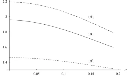
findings of our Theorem 4.1 we now find that the rootk1∈(˜k1,ˆk1), where

ˆ k1=−µ+γλm¯ σ2 + sµ µ+γλm¯ σ2 ¶2 +2(r+λ) σ2

denotes the positive root of the characteristic equation σ2_k2_{+ 2(}_µ₊_γλm₎_k₌

2(r+λ), and ˜ k1=−µ+γλm¯ σ2 + sµ µ+γλm¯ σ2 ¶2 +2r σ2

(28)

denotes the positive root of the characteristic equationσ2_k2₊₂₍_µ₊_γλm₎_k_{= 2}_r_.

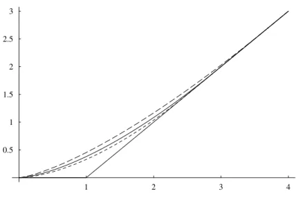
Consequently, we observe that in the present setting e˜k1x_sup y≥x n e−k˜1y_g₍_y₎ o ≤ek1x_sup y≥x © e−k1y_g₍_y₎ª_≤_eˆk1x_sup y≥x n e−ˆk1y_g₍_y₎ o

provided that the maximum exists. Moreover, given that in the present case ˜ ψθ(x) =eKθx, where Kθ=−µ+γλm¯ σ2 + sµ µ+γλm¯ σ2 ¶2 +2θ σ2

we observe that argmax{e−k1y_g₍_y₎_}_{= argmax}_{_e−Kθy_g₍_y₎_}_{whenever the} iden-tity

θ=r+λ

Z (0,∞)

(1−eγzk₎_m₍_dz₎ ₍₂₃₎

holds. This observation is important since it demonstrates that in the present case both the value as well as the optimal stopping rule of the optimal stop-ping problem (3) of the underlying jump diffusion coincides with the value and stopping rule of the associated stopping problem of a continuous diffusion by properly adjusting the discount rate. Hence, our results indicate that whenever the value of the optimal policy admits the representation (22) the jump-risk can be viewed as a discount rate effect as characterized by the identity (23). More precisely, whenever the value of the optimal policy admits the representation (22) we have that ˜Vθ(x) =V(x) by choosing the discount rate according to the

identity (23).

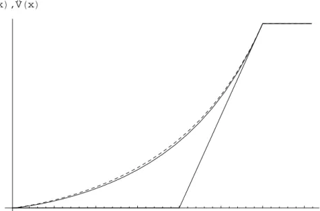
It is worth noticing that according to our general results the strict convexity of the increasing fundamental solution ek1x _{implies that increased volatility} _σ as well as higher jump-intensity λincreases the value of the optimal stopping policy and raises the optimal boundary at which the underlying jump-diffusion should be stopped. To see that this is indeed the case consider the mapping

¯ P(λ, σ, k) = (µ+γλm)k+1 2σ 2_k2₊_λ Z (0,∞) eγzkm(dz)−(r+λ). Standard differentiation yields that ¯Pσ(λ, σ, k) =σk2>0 and

¯

Pλ(λ, σ, k) =

Z (0,∞)

(29)

Therefore, the inequality ¯P(λ, σ,0) =−r <0, the limiting condition ¯P(λ, σ, k)↑

+∞ as k→ ∞, and the strict convexity of the function ¯P(λ, σ, k) imply that ∂k1/∂σ < 0 and ∂k1/∂λ < 0 and, therefore, that ∂ek1(x−y)/∂σ > 0 and

∂ek1(x−y)/∂λ >0 for allx≤y.

As a numerical illustration, consider thecapped option reward function g(x) = max{0, pmin(K, x)−qK},

where we assume p > q > 0 and K ≤ p

p−qk11 =: K0 to guarantee that g/ψ is maximized at K (if K > K0, the maximizer is an interior point of (0, K),

see Alvarez (1996) for a detailed analysis and interpretation in the continuous setting). As stated, in this caseg/ψattains a unique maximum value atx∗₌_K_,

which is a point of nondifferentiability for g. Assumption g1 is now satisfied and ifAg2 holds, the value of the optimal stopping problem is

V(x) =ek1x_sup y≥x © e−k1y_g₍_y₎ª₌      (p−q)K, x≥K ek1(x−K)₍_p₋_q₎_{K, x < K} (24) This is a continuous function, but its derivative has a discontinuity atx∗_:

lim x→x∗₋V 0₍_x_{) =}_k 1(p−q)K >0 = lim x→x∗₊g 0₍_x_{) = lim} x→x∗₊V 0₍_x₎_,

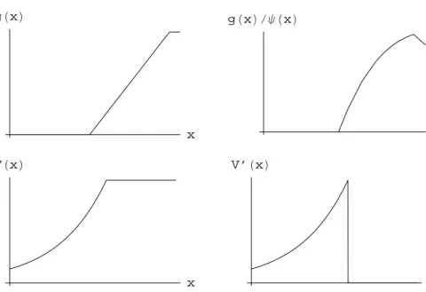
and there is no smooth pasting. The graphs of the reward function, the function g/ψ and the value and its derivative for p= 1, q = 0.5,r = 0.04, µ= 0.075, σ = 0.1, λ = 0.1, γ = −0.5, and K = 0.75·K0 (implying that k1 = 1.1463

and K0 = 1.7447) are shown in Figure 1 (for these values it can be checked

numerically thatAg2 holds).

6.2 Geometric Stochastic Dynamics

Geometric processes have been of paramount importance in mathematical fi-nance for several decades, with the most extensively used and well-known in-stance being the geometric Brownian motion St = s0exp{µt+σWt}, where σ >0 andW is a standard Wiener process. During the last decade, a consider-able amount of research has been done on geometric L´evy models

(30)

x VHxL x V’HxL x gHxL x gHxLΨHxL

Figure 1: The reward function g, the function g/ψ, the value function V and the derivative of the valueV0 _{for the capped option case}

where in addition to the deterministic drift and the Gaussian component there is a jump processJtin the exponent.

A geometric L´evy processY ={Yt}with a finite L´evy measureν=λmis a

jump diffusion whose dynamics are given by dYt=Yt− ( αdt+σdWt+λ Z S(m) γ(z)(N(dt, dz)−ν(dz)dt) ) , (26) where both the driftαand the diffusion coefficientσare assumed to be positive. Note that in this caseI=R+ and the explicit solutionYtequals

y0exp n ˜ αt+σWt+ Z t 0 Z S(m) ln(1 +γ(z)) ˜N(ds, dz)o. (27) where ˜α = α− 1

2σ2. To ascertain that X1 holds, we require that ˜α > 0.

For simplicity of exposition, we take γ(z) = −z and to guarantee that X2 is satisfied, we assume S(m) ⊆ (0,1). Furthermore, to ensure the finiteness of the value of the optimal stopping problem, we need to impose the integrability conditionα−r <0 (which is known in the literature on financial economics as