Probabilistic Structured Models for Plant Trait Analysis

(1)

Probabilistic Structured Models for Plant Trait Analysis

A DISSERTATION

SUBMITTED TO THE FACULTY OF THE GRADUATE SCHOOL OF THE UNIVERSITY OF MINNESOTA

BY

Farideh Fazayeli

IN PARTIAL FULFILLMENT OF THE REQUIREMENTS FOR THE DEGREE OF

DOCTOR OF PHILOSOPHY

ARINDAM BANERJEE

(2)

c

(3)

Acknowledgements

I would like to express my sincere gratitude to my advisor, Prof. Arindam Banerjee, for his continuous support of my PhD study and research. He has been a tremendous researcher, mentor, instructor, and role model. His patience, motivation, enthusiasm, immense knowledge, and dedication to research encourage me to never give up and overcome difficult obstacles, and trigger me to grow as a research scientist. I have been extremely lucky to have him as my PhD advisor and will be forever thankful to him for introducing me to the wonders of scientific research.

I would like to thank Prof. Sudipto Banerjee, Prof. Daniel Boley, Prof. Vipin Kumar, and Prof. Peter B. Reich for being my dissertation committee members. I am also grateful to my collaborators Jens Kattge, Peter B. Reich, Franziska Schrodt, Habacuc Flores-Moreno, Abhirup Datta, Anuj Karpatne, Ethan Butler, Kirk Whythers, and Ming Chen. It was a pleasure to work and collaborate with them on the plant trait analysis throughout almost four years of the project.

I will miss my long discussion sessions and interactions with all my labmates and friends: Amir Taheri, Andre Goncalves, Hardik Goel, Huahua Wang, Igor Melnyk, Jamal Golmohammady, Karthik Subbian, Konstantina Christakopoulou, Miao Fan, Nicholas Johnson, Puja Das, Qilong Gu, Robert Giaquinto, Shaozhe Tao, Sheng Chen, Sijie He, Soumyadeep Chatterjee, Vidyashankar Sivakumar, Xiaoli Liu, Yingxue Zhou. My special appreciation goes to my family for their endless love in my whole life. It would have been impossible for me to finish this work without their encouragement, understanding, support, and help.

I owe my loving thanks to my husband and best friend, Hamed Kajbaf, for all the emotional support, camaraderie, enthusiasm, caring, and helping me to get through the difficult times.

(4)

Dedication

To my parents and Hamed.

(5)

Abstract

Many fields in modern science and engineering such as ecology, computational bi-ology, astronomy, signal processing, climate science, brain imaging, natural language processing, and many more involve collecting data sets in which the dimensionality of the datapexceeds the sample size n. Since it is usually impossible to obtain consistent procedures unless p < n, a line of recent work has studied models with various types of low-dimensional structure, including sparse vectors, sparse structured graphical models, low-rank matrices, and combinations thereof. In such settings, a general approach to estimation is to solve a regularized optimization problem, which combines a loss func-tion measuring how well the model fits the data with some regularizafunc-tion funcfunc-tion that encourages the assumed structure.

Of particular interest are structure learning of graphical models in high dimensional setting. The majority of statistical analysis of graphical model estimations assume that all the data are fully observed and the data points are sampled from the same distribu-tion and provide the sample complexity and convergence rate by considering only one graphical structure for all the observations. In this thesis, we extend the above results to estimate the structure of graphical models where the data is partially observed or the data is sampled from multiple distributions. First, we consider the problem of estimat-ing change in the dependency structure of twop-dimensional models, based on samples drawn from two graphical models. The change is assumed to be structured, e.g., sparse, block sparse, node-perturbed sparse, etc., such that it can be characterized by a suit-able (atomic) norm. We present and analyze a norm-regularized estimator for directly estimating the change in structure, without having to estimate the structures of the individual graphical models. Next, we consider the problem of estimating sparse struc-ture of Gaussian copula distributions (corresponding to non-paranormal distributions) using samples with missing values. We prove that our proposed estimators consistently estimate the non-paranormal correlation matrix where the convergence rate depends on the probability of missing values.

In the second part of thesis, we consider matrix completion problem. Low-rank

(6)

ommendation systems. However, most of the existing matrix completion methods only provide a point estimate of missing entries, and do not characterize uncertainties of the predictions. First, we illustrate that the the posterior distribution in latent factor models, such as probabilistic matrix factorization, when marginalized over one latent factor has the Matrix Generalized Inverse Gaussian (MGIG) distribution. We show that the MGIG is unimodal, and the mode can be obtained by solving an Algebraic Riccati Equation equation. The characterization leads to a novel Collapsed Monte Carlo inference algorithm for such latent factor models. Next, we propose a Bayesian hierar-chical probabilistic matrix factorization (BHPMF) model to 1) incorporate hierarhierar-chical side information, and 2) provide uncertainty quantified predictions. The former yields significant performance improvements in the problem of plant trait prediction, a key problem in ecology, by leveraging the taxonomic hierarchy in the plant kingdom. The latter is helpful in identifying predictions of low confidence which can in turn be used to guide field work for data collection efforts.

Finally, we consider applications of probabilistic structured models to plant trait analysis. We apply BHPMF model to fill the gaps in TRY database. The BHPMF model is the-state-of-the-art model for plant trait prediction and is getting increasing visibility and usage in the plant trait analysis. We have submitted a R package for BHPMF to CRAN. Next, we apply the Gaussian graphical model structure estimators to obtain the trait-trait interactions. We study the trait-trait interactions structure at different climate zones and among different plant growth forms and uncover the dependence of traits on climate and on vegetation.

(7)

6 Matrix Completion with Hierarchical Side Information 77 6.1 Introduction . . . 77 6.2 BHPMF . . . 78 6.2.1 Model specification . . . 79 6.2.2 Sampling U . . . 79 6.2.3 Sampling V . . . 80 6.2.4 BHPMF Inference . . . 81 6.3 Experimental Results . . . 82 6.3.1 Dataset . . . 82 6.3.2 Baselines . . . 83 6.3.3 Methodology . . . 84 vii

(10)

6.4 Multiple Inheritance BHPMF . . . 90

III Application 93 7 Trait-Trait Interactions across Climate Zones 94 7.1 Statement of Contribution of co-authors . . . 94

7.2 Introduction . . . 94 7.3 Method . . . 98 7.3.1 Data . . . 98 7.3.2 Analysis . . . 100 7.3.3 Results . . . 103 7.4 Discussion . . . 105

7.4.1 Connectivity across all terrestrial plants . . . 106

7.4.2 Trait connections across growth forms and climate regions . . . 107

7.4.3 Modularity . . . 108

7.4.4 Modularity across climate regions and growth forms . . . 108

7.4.5 Modularity across a precipitation and a temperature gradient . . 109

7.4.6 Plant trait network analyses on a precipitation and temperature gradient holding the other environmental variable constant across each gradient . . . 111

7.4.7 Calculation of latent variables using a sparse precision matrix and low rank matrix . . . 112

8 Conclusion 126 References 129 Appendix A. Direct Change Estimation Appendix 152 A.1 Background and Preliminaries . . . 152

A.1.1 Generic Chaining . . . 154

A.2 Regularization Parameter . . . 156

A.3 RSC condition . . . 166

(11)

List of Tables

4.1 Edges dicovered by DoPinG and mGlasso on Climate Data. > denotes the number of edges in DoPinG graph but not in mGlasso graph. < is on the contrary. . . 56 5.1 Time Comparison of CMC and MCMC on different datasets. At each

step of MCMC, rows ofU and V can be sampled in parallel denoted by MCMC parallel. The running time is reported over 1000 steps for both methods where MCMC has 200 effective samples and CMC has 1000 effective samples. Note that the effective number of samples of MCMC is less than 1000 and more steps is required to obtain enough samples. The number of iterations for convergence of CMC is much less than 1000 (Figure 5.5). . . 76 6.1 ID, name, percentage of missing entries (%) and definition of the

respec-tive trait. . . 84 6.2 RMSE of Species Mean, PMF, HPMF and BHPMF. Latent dimension

k=15 for matrix factorization methods. . . 85 7.1 Examples of studies focused on multi-organ, multi-trait datasets. When

several plant group classifications were used, a semicolon divides them. The numbers next to the name of the organs included the study in the Organs column refers to the number of traits per organ. For more details on these studies see Appendix S. . . 114

(12)

trait values. Sample sizes (n) of the gap filled and original database are the same to ensure they are comparable. To test whether the gap-filling algorithm had an effect on trait-trait correlation we used a subset of 470769 observations from TRY for five traits (leaf area, SLA, leaf n, plant height and seed mass). First we ran the gap filling algorithm on this dataset. Then using standardize major axis analyses we compared the trait-trait correlations of a dataset only using observed values vs. the exact same observations only using gap filled values. The sample sizes for these trait-trait correlations varied between 1738 for the leaf N-seed mass correlation to 63846 records for the SLA-leaf area correlation. Overall, the difference in the slope value of the trait-trait correlation between the two types of data (gap-filled vs original) ranged from 0.0005 to 0.06, and in the case of the intercepts it varied between 0.006 and 0.11. . . 115 7.3 Modules of non-woody and woody species across climate regions. The

pipe character ‘|’ separates individual modules. Traits across modules may be connected (see Figure 7.3), however they tend to be more con-nected with other traits within the modules than with traits outside the module. . . 115 7.4 Trait connections that are robust (i.e. common across groups) across

growth forms and climate regions and proposed mechanisms that main-tain this connection. The range of R2values observed across growth form, and then by growth form across climate regions in this study is provided from the second to fourth columns. We provided mechanism proposed to maintain these trait connection as well as specific hypothesis about this mechanism (Details column). . . 116 7.5 Trait-trait correlations (r) and precision matrix values (ω) for all land

plants, woody and non-woody species. . . 117 7.6 Woody species trait-trait correlations (r) and precision matrix values (ω)

across climate regions . . . 118 7.7 Non-woody species trait-trait correlations (r) and precision matrix values

(ω) across climate regions . . . 119

(13)

into five different climate regions. Analyses were ran using (A) mass-based, and (N) area based leaf nutrient content (N, and P). . . 121 7.9 Connectivity (i.e. Edge density ) and modularity of plant trait networks

for woody and non-woody species across five different climate regions. Analyses were ran using (A) mass-based, and (N) area based leaf N and P content. . . 121 7.10 Number of present edges and modularity of plant trait networks and

modularity for temperature and precipitation gradients. n refers to the number of species in each category. . . 123 7.11 Trait centrality (i.e. Degree) for woody angiosperms, non-woody forbs

and non-woody monocots across a precipitation and temperature gradi-ent, holding the other climate variable constant (see Section 7.4.6). . . . 123

(14)

List of Figures

1.1 TRY db (https://www.try-db.org/): (a) A snapshot of TRY db where rows are plants and columns are traits. Blues denote the missing data. It is almost blue. (b) Spatial coverage of measurement sites for plant traits in the TRY db (blue), and the contributing institutes (red) [101]. . . 5 1.2 Presenting the graphical structure ofθ1,θ2 and the change δθ=θ1−θ2

where blue denotes the common edges betweenθ1 and θ2, red edges are only present in θ1 and green edges are only present in θ2. a) In this scenario, bothθ1 and θ2 are sparse that can be estimated correctly even in the low sample setting. Hence, an indirect approach can efficiently estimate the change δθ. b) In this scenario, θ1 and θ2 are both dense, butδθ is sparse. Since θ1 and θ2 can not be estimated correctly in the low sample setting, a direct estimator is a more efficient and consistent approach to estimate the change. . . 8

(15)

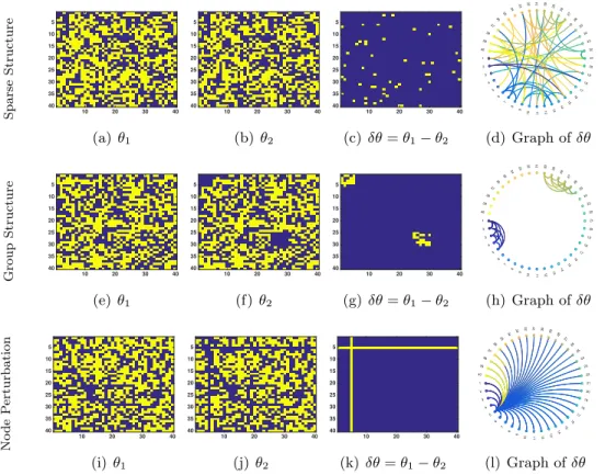
and second columns are the adjacency matrix for two graphical models at different conditions (θ1 and θ2) where blues denotes zero (missing edges). Third columns shows the change between two adjacency matrices (δθ=θ1−θ2), and last column shows the graphical structure ofδθ. Each row presents an example of δθ with different structures. In all three scenarios, both θ1 and θ2 are pretty dense. First row shows the sparsity structure of δθ (a few edges has been changed). Second row presents the group sparsity structure (the connection of two blocks of nodes has been changed). Last row shows the node perturbation structure (the connections of node 5 to all other nodes has been perturbed). The goal of generalized direct change estimation is to estimateδθ(the third column) under different structure without estimatingθ1 and θ2. . . 9 1.4 In this example, the matrix X is a tall matrix. All previous algorithms

in the literature [21, 22, 117, 144, 174, 175], require either estimating or sampling both latent matrices U or V. The motivation behind our collapsed Monte Carlo inference is to marginalize the tall matrix U and infer the parameters only based on the smaller matrixV. . . 11 1.5 BHPMF Schematic and Markov blanket ofnthrow ofU(2)_,_u(2)

n , is shown

in the red box. In spite of the size of the model, the Gibbs sampler is efficient since the Markov blanket is small and independent of the number of levels. . . 12 1.6 Trait-trait interaction as a function of temperature (x-axis) and

rain-fall (y-axis). Edges represent the conditional dependency between traits (nodes). . . 13

(16)

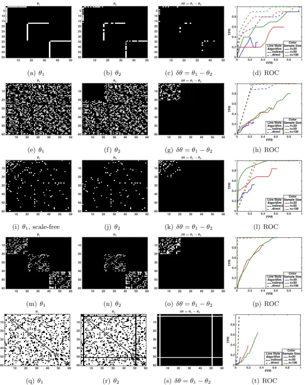
3.1 First rowδθ has a sparse structure (L1norm) andθ1 has 3 disconnected star graphs. Second, third, and forth rowsδθ∗ has group sparse structure (group sparse norm) where θ₁∗ has a random graph structure in second row, scale-free structure in third row, and block structure in forth row. Last rowδθ∗ has two perturbed norm (Node perturbation) and θ₁∗ has a random graph structure. Blacks in heatmaps denotes zeros. ROC curve for different structures show in the last column. Direct approach has a better ROC curve for all structures except with scale-free structure ofθ∗₁. 39 4.1 (a,b) ROC curves without projection ( ˆSneed not be positive semi-definite),

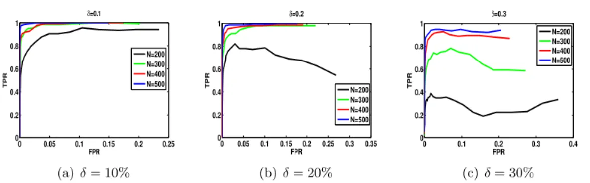
(c,d) ROC curves with projection ( ˆS is positive semi-definite) with n= 200 and under different missing probabilities (δ= 0.1−0.3). By increas-ing number of observed data (smallerδ), the ROC curve approaches the ROC curve of no-missing data (δ = 0). . . 52 4.2 ROC curve withδ = 0.1,0.2,0.3,p = 100, and different number of

sam-ples (n). For a fixed value of δ, with increasing number of samples, the higher TP rates is obtained. . . 53 4.3 ROC curve of mGlasso withn= 200 and different missing probabilities.

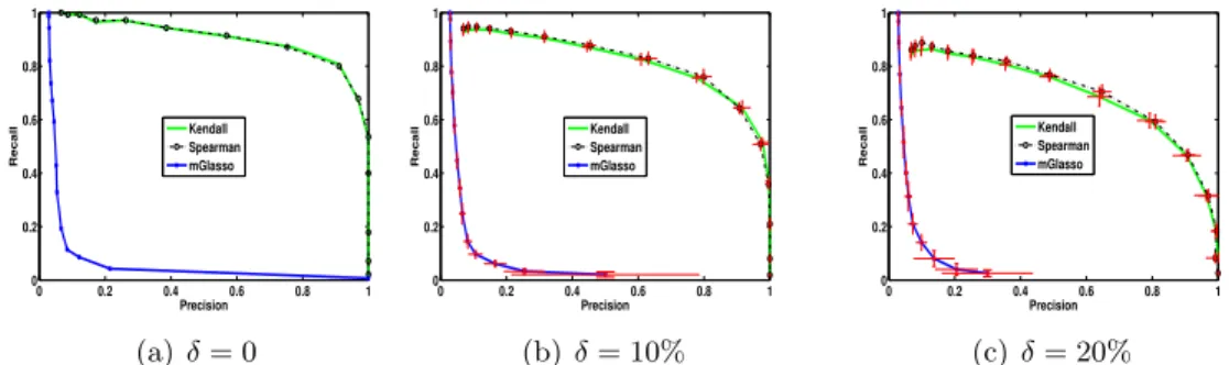
mGlasso has a worse performance on non-Gaussian data compared to DoPinG (Figure 4.1). . . 54 4.4 Precision and Recall Curve with different δ. DoPinG is significantly

better than mGlasso for non-Gaussian data. . . 55 4.5 The graph discovered by DoPinG and mGlasso. . . 56 5.1 An illustration of bad proposal distribution in importance sampling. Let

p(x) =h∗(x)g∗(x)/Zp ∝h(x)g(x). Neither h(x) = h∗(x)/Zh norg(x) = g∗(x)/Zg are a good candidate proposal distribution since their modes

are far away from the one ofp(x). . . 59 5.2 (a,b) Comparison of different proposal distribution (a) Wishart (W) and

(b) Inverse Wishart (IW) for sampling mean of MGIG1(Ψ,Φ, ν) where Λ∗ is the mode of M GIG. The blue curves are the proposal distribu-tion defined in [229, 233] which can not recover the mode of theMGIG

distribution. . . 63

(17)

5.3 Illustration of 2-dimensional (a) distribution (b-f) and different proposal distributions where (b-e) are the proposal described in this chapter where Λ∗ is the mode of M GIG and (f) is the proposal de-fined in [229, 233]. the proposal distribution dede-fined in [229, 233] (f) can not recover the mode of theMGIG distribution (a). (g) Density of

MGIG₂(Ψ,Φ, ν) for 1000 samples generated by each proposal distribu-tion is calculated. More than 90% of samples generated by the previ-ous proposal distribution in [229, 233] (IW(ψ,−2ν)) have zero MGIG

density leading to ESS = 40. Whereas, the new proposal distribution

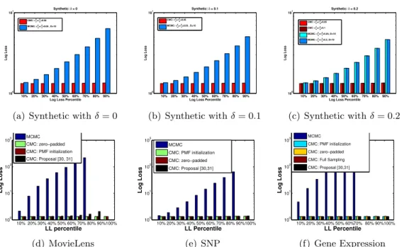
IW(23Λ∗,20) has the ESS = 550 which has a very similar shape to the targetMGIG distribution. . . 64 5.4 Log loss (LL) of CMC and MCMC for different log loss percentile on

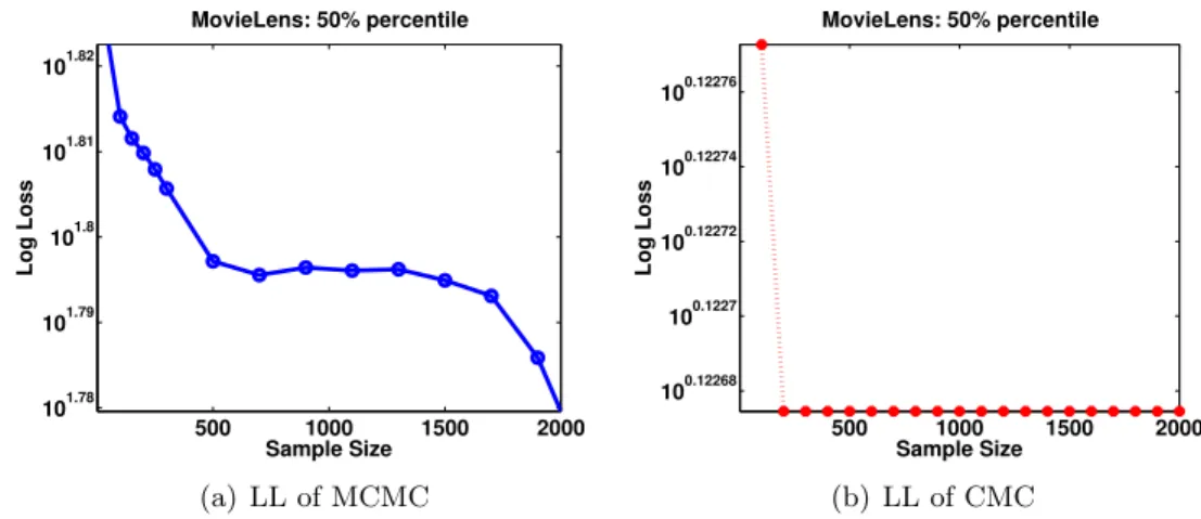
different datasets presented in the log scale (δ denotes the missing pro-portion). CMC consistently achieves lower LL compared to MCMC. LL of MCMC increases exponentially (linearly in log scale) by adding data points with higher log loss. Proposal in [30,31] achieved infinity LL for MovieLens. Empty bar represents infinity LL (e.g. 90% and 100% per-centile in (d) . . . 73 5.5 LL of CMC and MCMC for different sample size of MovieLens data in

the log scale. LL of both CMC and MCMC is decreasing by adding more samples. LL of MCMC is in magnitude 10 times more than CMC. . . . 74 5.6 Density of CMC and MCMC for several data input on MovieLens data.

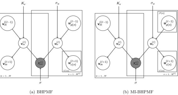
CMC provide distributions with lower LL compared to MCMC e.g. in (a) LL of MCMC is -Inf whereas LL of CMC is -1.78. . . 75 6.1 (a) BHPMF and (b) MI-BHPMF schematic at level (`). In spite of the

size of the model, the Gibbs sampler is efficient since the Markov blanket is small and independent of the number of levels. MI-BHPMF supports multiple inheritance. . . 78

(18)

tions. Block-wise sampler outperforms others. b) BHPMF for all traits and with the inverse of prediction confidence (Std) on the x-axis and the prediction error (RMSE) on the y-axis. The errors are small (more accurate) when the Std is small (more confident). . . 86 6.3 a,b,e) Spatial coverage of all observation, the highest and lowest confident

group. Trait measurements in China or south Africa are more frequent in the uncertain groups (e). Additional measurements in the densely covered regions like China may improve the accuracy. . . 88 6.4 Scatter plots for pairs of traits (a) on observed true test data, (b)

pre-dicted by HPMF, and (c) prepre-dicted by BHPMF. BHPMF and PHMF preserve true trait correlations. . . 89 6.5 MI-BHPMF for all movies with the inverse of prediction confidence

(stan-dard deviation) on the x-axis and the prediction error (RMSE) on the y-axis. The errors are small (more accurate) when the standard deviation is small (more confident). . . 91 6.6 BHPMF for each of the 13 traits with the inverse of prediction confidence

(standard deviation) on the x-axis and the prediction error (RMSE) on the y-axis. The errors are small (more accurate) when the standard deviation is small (more confident). . . 92 7.1 Hypothetical scenarios when determining the conditional dependency

among correlated traits. (a) Observed correlation between trait y and traitx, when the effect of traitz has not been considered (dashed gray lines). (b) Conditional dependence between traitxand traity even after considering trait z, suggesting dependency between trait x and trait y. (c) Conditional independence between trait y and trait x, once trait z

has been considered, suggesting that the correlation betweenxandywas indirectly mediated throughz. . . 101 7.2 Connections between multiple traits across organs (leaves in greens, stems

in browns and seed in red) using mass units for leaf N and P content. (A) all terrestrial plants, (B) non-woody species and (C) woody species. 111

(19)

browns and seed in red) for woody (A-E) and non-woody species (F-J) in (Tr) Tropical, (Te) Temperate, (Ar) Arid, (Co) Cold, and (Po) Polar environments. Environment types were derived using the Kppen Climate Zones classification system (Peel et al., 2007; see methods). . . 112 7.4 Connections between traits across organs (leaves, stems and seed) using

area units for leaf N and P content. (A) All terrestraial plants included in this study, (B) No-woody species, (C) Woody species. . . 120 7.5 Connections between traits across organs (leaves, stems and seed) for

woody (A-E) and non-woody species (F-J) across a climate gradient and using area-based measurements of leaf N and P content. The climate regions are Tr Tropical, Te Temperate, Ar Arid, Co Cold, Po Polar. . . 120 7.6 Connections among traits across multiple organs for woody angiosperms

across a temperature gradient, holding precipitation between 0-500 mm. 122 7.7 Connections among traits across multiple organs for forbs across a

tem-perature gradient, holding precipitation constant between 0-500 mm. . . 122 7.8 Connections among traits across multiple organs for woody angiosperms

across a precipitation gradient, holding temperature between 10-20 C. . 124 7.9 Connections among traits across multiple organs for non-woody (A-C)

forbs and (D-E) monocots across a precipitation gradient, holding tem-perature constant between 10-20 C. . . 124 7.10 Interaction between variables may depend on latent (or unmeasured)

vari-ables. For example, in graph a. Wet Street and Wet Grass are condi-tionally dependent without observing the Rain variable, but they become conditionally independent after observing the Rain Variable (b). Dash lines present the direct edges that cannot be obtained without consider-ing the unmeasured variables. In another example (c), in the presence of a sprinkler the interaction structure may change to the following graph. 125

(20)

Chapter 1

Introduction

Many fields in modern science and engineering such as ecology [64, 71], computational biology [12, 39, 184, 232], astronomy [13, 193], signal processing [30, 47, 204], climate science [59, 178], brain imaging [61, 120], natural language processing [10, 80], and many more involve collecting data sets in which the dimensionality of the data p exceeds the sample size n. For example, in computational biology, usually the expression level of thousands genes for about hundreds of patients are measured. A common problem is then to estimate the gene-gene interaction networks which requires estimating p = thousands×thousands interactions from only hundreds samples (i.e.,n < p). In another example, consider plant traits analysis where on average three out of 1000 traits are measured (i.e., more than 95% of trait measurements are missing). A typical goal is to fill the gaps in the plant traits matrix for about 1 million (1M) plants which requires estimatingp= 1000×1M trait values from only a small fraction of measured traits.

In settings where the number of parameters is large relative to the sample size, the use of well studied classical approaches such as least squares regression is problematic since such methods need n > p to be statistically and/or computationally meaningful. In the high dimensional settings, sparse models, or in general constrained structurally models, are usually preferred due to easier interpretation and more accurate and con-sistent results. For example, a small number of genes may constitute a signature for disease, very few parameters may be required to specify the correlation structure in a time series, or a sparse collection of geometric constraints might completely specify a molecular configuration. Such low-dimensional structure plays an important role in

(21)

making high dimensional problems well-posed.

1.1 Structured Graphical Models

The past decade has seen considerable advances in high-dimensional sparse and struc-tured models which continue to stay effective under ‘low sample’ settings, even when the number n of samples is smaller than the ambient dimensionality p of the model, i.e., n ≤ p. Such models includes sparse and structured sparse regression models (e.g., Lasso, group Lasso) [186, 201, 236], matrix completion models under low rank assumptions[38, 104, 150, 166], and sparse structure learning of graphical model [15, 100, 140, 164, 165, 228]. Due to the preliminary success in certain application do-mains, there have been increasing attempts to apply such sparse/structured mod-els to scientific problems such as in climate science, brain sciences, ecology, and ge-nomics [43, 71, 231, 239, 240].

To control the structure and complexity of the model, often regularization terms have been added to the objective function. For instance, in application to linear models, the Lasso or basis pursuit approach [48, 201] is based on a combination of the least-squares loss with `1-regularization which has been widely applied for feature selection. Similar approaches have been applied to generalized linear models, resulting in more general (non-quadratic) convex programs with `1-constraints. Several types of regularization have been used for estimating matrices, including standard `1-regularization, a wide range of sparse group-structured regularizers, as well as regularization based on the nu-clear norm (sum of singular values). In high-dimensional settings, regularization serves two purposes: one statistical and the other computational. Statistically, regularization is essential: it prevents overfitting and allows us to design estimators that exploit latent low-dimensional structure in the data to achieve consistency. From the computational point of view, regularization improves the stability of the problem and often leads to computational gains.

In this thesis, we develop probabilistic models for matrix completion and structure learning of graphical models in high-dimensions and apply those advanced methods in plant trait analysis as an application. In certain settings, we focus on Bayesian graphical models since they can produce uncertainty quantified predictions, such as a distribution

(22)

over possible values rather than a point estimate; further, since graphical models are modular, combining different models together based on different sources of information can be conceptually straightforward. In this chapter, we start by a brief overview of structure learning of graphical models and low rank matrix completion models, followed by an introduction to the plant trait analysis. Finally, we present an overview of our contributions and developed models.

1.1.1 Structure Learning of Graphical Models

Probabilistic graphical models provides a mechanism for exploiting structure in com-plex distributions to describe them compactly, and in a way that allows them to be constructed and utilized effectively. These models use a graph-based representation where the nodes are the random variables in our domain, and the edges correspond to direct probabilistic interactions between them. If there is no edge between two nodes, then the corresponding variables are conditionally independent given all other variables. Often, we may not know the correct graph structure to use for modeling some collection of random variables. Then, it is natural to seek a good graph structure based on sample data. Learning the structures of graphical models have applications in several domains such as learning the gene-gene (or protein-protein) interactions from the gene expression levels data [78, 121], learning the brain neural connectivity [93, 146], and inferring the interaction network among stock markets [82, 84, 88].

In recent years, considerable effort has been invested in obtaining an accurate es-timate of sparse structure of graphical models including learning graph structure of Gaussian graphical models [15, 76, 100, 140, 165, 36, 35, 130, 235], Ising graphical mod-els [164], and multivariate Poisson graphical modmod-els [228]. Further, the Gaussian graph-ical models are generalized to Gaussian copula graphgraph-ical models which can automati-cally detect potentially nonlinear but monotonic relationships, and correctly identify the nonparametric correlations [128, 227]. The sparse graph strurcture learning have been extended to handle data with missing values in the data [126, 192, 136, 134, 103, 214], which often occur in real world applications, e.g., drop-outs of sensors in a sensor net-work or missing measurements of temperature or rain in climate.

Throughout the literature, for the high dimensional regime, the non-asymptotic up-per bounds on the estimation error has been extensively studied [15, 100, 140, 164,

(23)

165, 228, 36]. In a high dimensional setting, accurate estimation of the graphical struc-ture depends on how sparse the true graphical strucstruc-ture is. However, the majority of statistical analysis of graphical model estimations assume that all the data points are sampled from the same distribution and provide the sample complexity and convergence rate by considering only one graphical structure for all the observations [36, 164, 165]. New analysis is required to extend the consistency analysis of graphical models when observations draw from multiple distributions.

1.1.2 Low-rank Matrix Completion

Matrix completion is another challenging problem that arise in high dimensional set-tings. Matrix completion has been extensively studied in the recent literature and have been shown to be successful in a variety of settings [2, 106, 117, 162, 174, 175, 188]. To illustrate the problem statement, consider the collaborative filtering problem of estimat-ing how N users will rate M movies. Clearly, we will have p=N ×M parameters to estimate fromnobserved ratings. That is, we wish to recover estimates for all possible pairs of movie and user ratings based on only a small fraction of rated films.

The classical statistical setting would require that a small number of entries are missing in order to make an accurate prediction of the ratings. In essence, we would require that majority of users to watch and record a rating for majority of movies, which would be very impractical. However, several modern problems, e.g., recommendation systems, plant traits, work with “mostly missing” matrices where more than 95% data is missing. Intuitively, if we only observe a small fraction of the entries, then there are an infinite number of matrices that can fit the same data observations. In general, there is no way to overcome this unless we impose an implicit structural constraint on the parameter set to reduce the effective size of the parameter space.

In most settings, low rank structural constraint has been imposed to the parameter set, since usually various users (and movies) share similar characteristics, hence users (and movies) can be represented in a low dimensional space. In general, the given sparse matrix X∈RN×M is approximated by a low-rank matrix ˆX =U VT whereU ∈RN×D and V ∈ _RM×D_{. The latent factors} _u

n ∈ RD, for each row n, and the latent factors

vm ∈RD, for each column m of matrixX are estimated, usually based on alternating optimization [97, 106]. Once the latent factors have been estimated, the inner product

(24)

(a) TRY Sparsity

TRY database, status 04.2012

(b) TRY spatial coverage

Figure 1.1: TRY db (https://www.try-db.org/): (a) A snapshot of TRY db where rows are plants and columns are traits. Blues denote the missing data. It is almost blue. (b) Spatial coverage of measurement sites for plant traits in the TRY db (blue), and the contributing institutes (red) [101].

of un and vm gives the prediction for the missing entryxnm.

Such methods broadly come in two flavors—from an optimization perspective usually based on a rank or nuclear-norm constraints [176, 225], or, using Bayesian models based on latent factors [174, 175]. Several important variants of such models have been inves-tigated [4, 117, 162, 174, 175, 188], including probabilistic matrix factorization (PMF) and its Bayesian generalizations [174, 175], as well as generalizations to probabilistic tensor factorization [49, 196, 226].

1.2 Plant Trait Analysis

We apply the developed probabilistic structured models to the analysis of plant traits. Plant traits are morphological, anatomical, biochemical, physiological or phenological features of individuals, their component organs or tissues [101]. Examples of traits include the nitrogen content of leaves, leaf area, and plant height. Trait distributions vary across different environmental conditions (e.g., temperature, precipitation, soil moisture), within evolutionary history, and among different species. Understanding trait variation and distribution at local and worldwide spatial scales is an important key to maintain biodiversity and ecosystem functional services (e.g., agricultural and forest productivity, regulation of atmospheric CO2), and predict the adaptation of planet to human activities and climate change.

(25)

To facilitate plant trait analysis, the TRY project (www.try-db.org) was launched in 2007 which brings together different trait databases in a central repository [101]. The TRY database has become the world’s largest trait database (covering 1000 traits and 2.1 million plants) and one of the most widely used resources for the ecological community. The TRY database in combination with the recent progress in machine learning provides a unique opportunity to study trait variation and distribution. Nevertheless, we are confronted with two key challenges: (1) Trait sparsity: while unprecedented in coverage, the TRY database is highly sparse (lacking most of the trait information. On average, only three out of 1000 traits are characterized for each individual plant (Figure 1.1(a)). As a result, incorporating the rich information provided by traits in understanding the adaptation of terrestrial ecosystems to climate changes remain difficult; (2) Spatial sparsity: with respect to spatial coverage at global scale, even 2.1 million individual plants provide a sparse coverage (Figure 1.1(b)).

The goal of this thesis is to address the above challenges and analyze plant trait data by proposing novel machine learning models. My main research contributions can be divided into two core components, respectively focusing on developing models (1) to provide trait predictions at individual plant level by incorporating plant taxonomic hierarchy (gap filling) and (2) to provide trait characterization in a given context e.g., climate, soil type, phylogeny, etc., in which they are considered (contextual trait-trait interactions). Understanding trait-trait relationships and trait-environment relation-ships can help on providing more explicit representation of ecosystem properties, and a more detailed and dynamic representation of trait variation.

TRY database has more than 99% of the entries missing (Figure 1.1(a)). At a high level, the data are similar to that in a recommendation system, with plants corre-sponding to users and plant traits correcorre-sponding to items, e.g., movies. Thus, for the plant-trait gap filling problem, one can use a suitable low-rank model, such probabilistic matrix factorization (PMF) and variants [5, 174, 175, 241]. The performance of models such as PMF on such plant trait gap filling problems [183] is sobering! To understand the reason, note that plants belong to species, and for gap-filling one can simply use the species mean for that trait, e.g., species mean for SLA, leaf N, leaf C, etc. The species mean sets an extremely competitive baseline for any model to beat, and in fact

(26)

substantially outperforms models such as PMF [71, 179, 183]. From a scientific per-spective, the species mean does not constitute an interesting prediction, since it entirely misses out on within species variation of plant traits, the so-called intra-specific vari-ability [6, 53]. Understanding such intra-specific varivari-ability, i.e., how plants adjust their traits under different environmental/climatic conditions, is of great scientific interest, and holds critical clues regarding the adaptability of the terrestrial ecosystem under a changing climate.

1.3 Overview and Contributions

In the first half of this thesis, we study structure learning of graphical models. Here, we are interested in learning the graphical structure at different contexts and identify how the graphical structure is evolving under different conditions. For instance, identifying how gene-gene interactions changed from healthy to cancer tissues, learning the changes between brain connectivity in normal and Alzheimer’s patients, or learning the changes in the stock market dependency structures. Next, we develop a novel model to estimate the structure of graphical models in presence of missing data and provide the statistical recovery analysis for the proposed estimator.

In the second part of this thesis, we focus on low rank matrix completion problems. In particular, we provide a novel Monte Carlo inference for low rank matrix factorization such as probabilistic matrix factorization (PMF) and Bayesian principle component analysis (BPCA), and proposed a novel Bayesian hierarchical PMF (BHPMF) model that incorporate hierarchical side information.

Finally, we consider applications of probabilistic structured models to plant trait analysis. We apply BHPMF model to fill the gaps in TRY database. The BHPMF model is the-state-of-the-art model for plant trait prediction and is getting increasing visibility and usage in the plant trait analysis [64]. Next, we study the trait-trait interaction structure at different climate zones for different plant growth forms. We briefly explain our contribution for each task in below.

(27)

𝜃" 𝜃# 𝛿𝜃 (a)

!" !# $!

(b)

Figure 1.2: Presenting the graphical structure of θ1, θ2 and the change δθ = θ1−θ2 where blue denotes the common edges between θ1 andθ2, red edges are only present in

θ1 and green edges are only present inθ2. a) In this scenario, bothθ1 and θ2 are sparse that can be estimated correctly even in the low sample setting. Hence, an indirect approach can efficiently estimate the changeδθ. b) In this scenario,θ1 and θ2 are both dense, butδθis sparse. Sinceθ1 andθ2 can not be estimated correctly in the low sample setting, a direct estimator is a more efficient and consistent approach to estimate the change.

1.3.1 Generalized Direct Change Estimation

While structure learning in graphical models has been widely studied over the past decade, we focus on the problem of estimating changes in graphical model structure: given two sets of samples Xn1

1 ={x1i}ni=11 and X

n2

2 = {x2i}ni=12 respectively drawn from twop-dimensional graphical models with true parametersθ₁∗andθ₂∗, whereθ∗₁, θ₂∗∈_Rp×p_,

the goal is to estimate the changeδθ∗= (θ∗₁−θ∗₂). In particular, we focus on the situation when the change δθ∗ has structure, such as sparsity, block sparsity, or node-perturbed sparsity, which can be characterized by a suitable (atomic) norm [42, 145]. However, the individual model parameters θ₁∗, θ∗₂ need not have any specific structure, and they may both correspond to dense matrices. The goal is to get an estimateδθˆof the change

δθ∗ such that the estimation error ∆ = (δθˆ−δθ∗) is small. Such change estimation has potentially wide range of applications including identifying the changes in the neural connectivity networks, the difference between plant trait interactions at different climate conditions, and the changes in the stock market dependency structures.

One can consider two broad approaches for solving such change estimation problems: (i) indirect change estimation, where we estimate θb₁ and θb₂ from two sets of samples

separately and obtain δbθ= (θb₁−θb₂), or (ii)direct change estimation, where we directly

(28)

Sparse Structure 10 20 30 40 5 10 15 20 25 30 35 40 (a)θ1 10 20 30 40 5 10 15 20 25 30 35 40 (b) θ2 10 20 30 40 5 10 15 20 25 30 35 40 (c)δθ=θ1−θ2 1 2 3 4 5 6 7 8 9 10 11 12 13 14 15 16 17 18 19 20 21 22 23 24 25 26 27 28 29 30 31 32 33 34 35 36 37 38 39 40 Show All Hide All (d) Graph ofδθ Group Structure 10 20 30 40 5 10 15 20 25 30 35 40 (e)θ1 10 20 30 40 5 10 15 20 25 30 35 40 (f) θ2 10 20 30 40 5 10 15 20 25 30 35 40 (g)δθ=θ1−θ2 1 2 3 4 5 6 7 8 9 10 11 12 13 14 15 16 17 18 19 20 21 22 23 24 25 26 27 28 29 30 31 32 33 34 35 36 37 38 39 40 Show All Hide All (h) Graph ofδθ No de P erturbation 10 20 30 40 5 10 15 20 25 30 35 40 (i)θ1 10 20 30 40 5 10 15 20 25 30 35 40 (j)θ2 10 20 30 40 5 10 15 20 25 30 35 40 (k) δθ=θ1−θ2 1 2 3 4 5 6 7 8 9 10 11 12 13 14 15 16 17 18 19 20 21 22 23 24 25 26 27 28 29 30 31 32 33 34 35 36 37 38 39 40 Show All Hide All (l) Graph ofδθ

Figure 1.3: Illustrating the idea behind generalized direct change estimation. First and second columns are the adjacency matrix for two graphical models at different conditions (θ1 andθ2) where blues denotes zero (missing edges). Third columns shows the change between two adjacency matrices (δθ=θ1−θ2), and last column shows the graphical structure of δθ. Each row presents an example ofδθwith different structures. In all three scenarios, both θ1 and θ2 are pretty dense. First row shows the sparsity structure ofδθ(a few edges has been changed). Second row presents the group sparsity structure (the connection of two blocks of nodes has been changed). Last row shows the node perturbation structure (the connections of node 5 to all other nodes has been perturbed). The goal of generalized direct change estimation is to estimateδθ(the third column) under different structure without estimating θ1 and θ2.

In a high dimensional setting, recent advances [36, 164, 165] illustrate that accurate estimation of the parameterθ∗of a graphical model depends on how sparse or otherwise structured the true parameter θ∗ is. For example, if both θ₁∗ and θ∗₂ are sparse and the samples n1, n2 are sufficient to estimate them accurately [164], indirect estimation of

δθˆshould be accurate (Figure 1.2(a)). However, if the individual parametersθ∗₁ and θ∗₂

(29)

sparsity (only a small block has changed) or node perturbation sparsity (only edges from a few nodes have changed) [145], direct estimation may be considerably more efficient both in terms of the number of samples required as well as the computation time (Figures 1.2(b) and 1.3).

Our Contributions: We consider general structured direct change estimation, while allowing the change to have any structure which can be captured by a suitable (atomic) norm R(·) [69]. Our work is a considerable generalization of the existing liter-ature which can only handle sparse changes, captured by the `1 norm [132]. In partic-ular, our work now enables estimators for more general structures such as group/block sparsity, hierarchical group/block sparsity, node perturbation based sparsity, and so on [14, 42, 145, 151]. The regularized estimator we analyze is broadly a Lasso-type estima-tor, with key important differences: the objective does not decompose additively over the samples, and the objective depends on samples from two distributions.

1.3.2 Gaussian Copula Precision Estimation with Missing Values

Recently, sparse gaussian graphical model structure estimators have also been general-ized to handle data with missing values [126, 192, 136, 134, 103], which often occur in real world applications, e.g., drop-outs of sensors in a sensor network or missing measure-ments of temperature or rain in climate. However, these sparse precision estimators rely on the Gaussian assumption, which may not be appropriate for non-Gaussian datasets. To deal with non-Gaussian data, H. Liu et al. [128] and L. Xue et al. [227] proposed Gaussian copula graphical models where existing estimators can be generalized to the non-paranormal distributions simply using one additional procedure, i.e., estimating nonparametric correlations. It has been shown that the nonparanormal is equivalent to Gaussian copula distribution [129, 206, 205]. Therefore, the estimated correlation ma-trix of the data after transformation can be plugged into the standard sparse graphical structure estimators with Gaussian assumption. The plug-in procedure can leverage existing theoretical results and achieve the optimal statistical rate of convergence for fully observed data.

Our Contributions: In a joint work with Huahua Wang, Soumyadeep Chatterjee and Arindam Banerjee, we generalize the Gaussian copula estimators to handle data with missing values [214]. In particular, our estimator uses two plugin procedures

(30)

Figure 1.4: In this example, the ma-trixX is a tall matrix. All previous al-gorithms in the literature [21, 22, 117, 144, 174, 175], require either estimat-ing or samplestimat-ing both latent matrices

U or V. The motivation behind our collapsed Monte Carlo inference is to marginalize the tall matrix U and in-fer the parameters only based on the smaller matrix V.

and consists of three steps: (1) estimate nonparametric correlations based on observed values, including Kendalls tau and Spearmans rho; (2) estimate the non-paranormal correlation matrix; (3) plug into existing sparse precision estimators. We show that the consistency rate of our copula estimators depends on the probability of missing values. Through experimental results, we illustrate the effect of sample size and percentage of missing data on the model performance. Experimental results show that our estimator is significantly better than Gaussian estimators.

1.3.3 Collapsed Monte Carlo Inference for Matrix Completion

In the second part of the thesis, we focus on the low rank matrix factorization models such as Probabilistic Matrix Factorization (PMF) or Bayesian Probabilistic Component Analysis (BPCA). For such models, the literature has considered approximate inference methods, such as variational inference [22], gradient descent optimization [117], MCMC [175], Laplace approximation [21, 144], or alternating optimization overU and V [174]. However, all the above inference methods require either estimating or sampling both latent matrices U or V which might not be efficient in several applications especially for tall or fat matrices (i.e.,M N orN M, figure 1.4).

Out contributions: We propose an efficient inference algorithm for such low rank models [70]. In particular, we show that after analytically marginalizing one of the latent matrices in PMF (or BPCA), the posterior over the other matrix has the Matrix Generalized Inverse Gaussian (MGIG) distribution. We illustrate that the MGIG

distribution is unimodal where the mode can be obtained by solving anAlgebraic Riccati Equation (ARE) [28]. This illustration yields to a novel Collapsed Monte Carlo (CMC)

(31)

U(1) V(1) N(1) M(1) U(0) V(0) U(2) V(2) N(2) M(2) U(3) V(3) N(3) M(3) U(4) V(4) N(4) M(4) U(5) V(5) N(5) M(5) X(5) phylogenetic group

family genus species plant

X(4) X(3) X(2) X(1) xn(2) uci(n)(3) up(n)(1) un(2) V(2) |C(n)| Figure 1.5: BHPMF Schematic and Markov blanket of nth _{row of} U(2)_,_u(2)

n , is shown in the red box.

In spite of the size of the model, the Gibbs sampler is efficient since the Markov blanket is small and inde-pendent of the number of levels.

inference algorithm for PMF. In particular, we marginalize one of the latent matrices, say U, and propose a direct Monte Carlo sampling from the posterior of the other matrix, sayV.

1.3.4 Matrix Completion with Hierarchical Side Information

A key limitation of most matrix factorization models is the inability to use the domain knowledge such as hierarchical side information. In fact, as we illustrate in Section 6.3.4, applying PMF (Probabilistic Matrix Factorization) model [174] which does not incorporate the plant taxonomic hierarchy leads to a performance worse than the simple algorithm MEAN which uses the domain knowledge [183]. Similar hierarchical structure shows up in other applications such as genre (or product type) hierarchy in movies (or products) recommendation. In fact, as we illustrate in Section 6.3.4, applying the PMF model [174] without using the hierarchical information, leads to a performance worse than the simple algorithm MEAN which uses the domain knowledge [183].

Our contribution: The sobering performance of PMF in the plant trait problem led us to take a close look at the domain knowledge available for the problem. An obvious choice was to somehow utilize the plant taxonomic hierarchy, i.e., species, genus, family, etc., in a hierarchical Bayesian low rank model (Figure 1.5). We have developed Bayesian Hierarchical PMF (BHPMF), which use a hierarchy of low rank matrix factorization models, one corresponding to each level of the taxonomic hierarchy, and each level serving as the prior to the next, going all the way down to individual plants [71]. Unlike PMF, the hierarchical low rank models outperformed the species mean baseline substantially, and even captured inter-trait correlations accurately although it was not designed to capture such second order structure explicitly.

(32)

Figure 1.6: Trait-trait interaction as a func-tion of temperature (x-axis) and rainfall (y-axis). Edges represent the conditional de-pendency between traits (nodes).

1.3.5 Trait-Trait Interactions across Climate Zones

Next, we apply the advances in structure learning of graphical models to estimate trait-trait interactions. Plant trait-traits are not independent of each other, hence an accurate description of their interactions gives us a clearer view of the links between physiologi-cal and morphologiphysiologi-cal traits [156, 161], differences between functional groups [155], im-proves our understanding of the effect of multivariate trait relationships on mechanisms of coexistence [108] and increases accuracy in modeling of ecosystem processes [215]. However, the relationship between traits often depend on the context, e.g., climate, soil type, phylogeny, etc., in which they are considered [3, 170, 169]. For example, two plants/plant types may be close according to phylogeny but in different climates can adapt different trait values.

Our contributions: In a joint work with Habacuc Flores-Moreno, Arindam Banerjee, and others [73], we study plant strategies integration focusing on environ-mental gradients and growth form (woody and non-woody) to answer our overall ques-tion - how does the interacques-tion between traits vary across plant types and environmental gradients? In essence, plants might have different strategies to solve similar environmen-tal dilemmas, and this difference in strategies could also be reflected in the integration among their traits [24]. Here, we first describe the trait-trait interaction network among plants, then we assess how does this trait network change across five broad climate re-gions (Tropical, Temperate, Arid, Cold and Polar) while accounting for differences in

(33)

(34)

Chapter 2

Related Work

2.1 Structured Learning of Graphical Models

Undirected graphical models, also known as Markov Random Fields (MRFs), are im-portant tools for representing multivariate probability distributions which are applied in a wide range of domains such as statistical physics [95], natural language processing [138], image analysis [57] and spatial statistics [172]. The undirected graphical models represent a joint distribution using clique-wise functions over an undirected graph which captures the dependencies among subsets of thep-dimensional discrete random variable

X = (X1, X2,· · ·Xp). Meaning that featureXiis conditionally independent ofXj given

all other variables if there is no edge in the associated undirected graph structure. The task of graphical model selection is to infer this underlying dependency graph based on data drawn from the corresponding distribution. This task is especially difficult in high-dimensional settings where the number of observations,nis typically even smaller than the number of variables p.

2.1.1 Gaussian Graphical Models

Meinshausen and Buhlmann proposed the neighborhood selection approach and applied the standard Lasso regression on Xj against Xjc to estimate nonzero entries in each

row [140]. In the same spirit, Yuan [235] applied the Dantzig selector version of this

(35)

regression to estimate Ω column by column. i.e. minkβk1 s.t. 1 nkX T jcX_j −X_jTcX_jck_∞≤τ. (2.1)

Cai et al. [36] further proposed an estimator called CLIME by solving a related opti-mization problem

ˆ

Ωn= argmin

Ω0

kΩk1 s.t.kΣˆnΩ−Ik∞≤τ. (2.2)

In practice, the tuning parameter τ is chosen via cross-validation. However the the-oretical choice of τ = CMn,plogp/n requires the knowledge of the matrix `1 norm

Mn,p = kΩk1, which is unknown. Later, Cai et al. introduced an adaptive version of CLIME which is data-driven and adaptive to the variability of individual entries of

ˆ

ΣnΩ−I [35].

Yuan and Lin first proposed to use penalized likelihood methods for estimating sparse precision matrices studied its asymptotic properties for fixed p asn→ ∞[236]. It is easy to see that under the Gaussian assumption the negative log-likelihood up to a constant, can be written as l(X(1), ..., X(n); Ω) = Tr( ˆΣnΩ) log det(Ω), where det(Ω)

is the determinant of Ω and Tr(.) is the trace function. To incorporate the sparsity of Ω, we consider the following penalized log-likelihood estimator with Lasso-type penalty

ˆ

Ωn= argmin

Ω0

Tr( ˆΣnΩ) log det(Ω) +λkΩk1, (2.3) where Ω0 means symmetric positive definite.

Rothman et al. analyzed the high-dimensional behavior of estimator (2.3) [173]. Assuming that spectra of Ω are bounded from below and above, the rates of convergence

p

(p+s) logp/nandp(1 +s) logp/nunder the Frobenius norm and spectral norm are obtained respectively with s being the number of nonzero off-diagonal entries. Lam and Fan studied a generalization of (2.3) and replace the Lasso penalty by general non-convex penalties such as SCAD to overcome the bias issue [112]. Ravikumar et al. applied the primal-dual witness construction to derive the rate of convergenceplogp/n

under the sup-norm which in turn leads to convergence rates in the Frobenius and spectral norms as well as support recovery under certain regularity conditions [165].

(36)

The results heavily depend on a strong irrepresentability condition imposed on the Hessian matrix Γ = Σ⊗Σ, where ⊗ is the tensor (or Kronecker) product. Both sub-Gaussian and polynomial tail cases are considered. However this method cannot be extended to allowing many small nonzero entries .

Although these sparse precision estimators are primarily designed to deal with fully observed data, recently, they have also been generalized to handle data with missing values [126, 192, 136, 134, 103], which often occur in real world applications, e.g., drop-outs of sensors in a sensor network or missing measurements of temperature or rain in climate. To deal with data with missing values, a variety of methods apply expectation maximization (EM) algorithms on imputed data, which are iterative methods but lack theoretical guarantees [126, 192]. Without using the EM algorithm, [134] employed projected gradient descent to solve a sequence of regression problems or PGlasso to estimate the sparse precision matrix of incomplete data. Theoretical guarantees are also established for the PGlasso estimator. M. Kolar and E. Xing introduced a simple plug-in procedure for incomplete data which simply applies existing estimators to the observed data by disregarding the missing values [103]. Such simple plug-in estimators for missing values can leverage existing theoretical results and thus still have similar sta-tistical guarantees, including rate of convergence and consistency. However, these sparse precision estimators rely on the Gaussian assumption, which may not be appropriate for real datasets which are usually non-Gaussian.

To deal with non-Gaussian data, H. Liu et al. [128] proposed Gaussian copula graphi-cal models where existing estimators can be generalized to thenon-paranormal distribu-tions simply using one additional procedure, i.e., estimating nonparametric correladistribu-tions. Non-paranormal distributions can be considered as a non-parametric extension of the normal distribution where suitable univariate monotone transformations of the covari-ates are jointly distributed as a multivariate Gaussian. It has also been shown that the nonparanormal is equivalent to Gaussian copula distribution [129, 206, 205]. Therefore, the estimated correlation matrix of the data after transformation can be plugged into the standard sparse precision estimators with Gaussian assumption. The plug-in pro-cedure can leverage existing theoretical results and achieve the optimal statistical rate of convergence. A similar procedure has also been studied independently by [227].

(37)

2.1.2 Ising Graphical Models

In literature, the problem of structure learning for discrete graphical models has at-tracted considerable attention due to both its importance and difficulty. Score-based approaches through a search procedure generate several candidate graph structures to be scored with a measure of the goodness of fit of the graph. However, the number of graph structures grows super-exponentially, and this problem is in general NP-hard [51]. A complication that arises in graphical model selection with discrete random variables is that the score metrics involve the partition function or cumulant function associated with the Markov random field which is usually computationally intractable [216]. It yields imposing a restricted search space such as directed graphical models [60], trees [52], or hypertrees [190] in the score-based approaches. A method for learning factor graphs based on local conditional entropies and thresholding is proposed in [1] which required the sample complexity of Ω(logp), but the computational complexity grows at least as quickly as O(pd+1_{) where}_d_{is the maximum degree in the graphical model.}

Ravikumar et al. proposed a new model for estimating Ising graphical model struc-ture based on`1regularized logistic regression [164]. In particular, the task of recovering of the signed edge vector is reduced to recovering of the signed neighborhood setN_±(r) for each node r, i.e., capturing both neighborhood structure N(r) and sign pattern for each noder. Given the exponential distribution of the Ising models, the structure of the conditional distribution ofXr given the other variables can be represented as a sigmoid

function. Thus, the variable Xr can be viewed as the response variable in a logistic

regression in which all of the other variables play the role of the covariates. Later, to impose the sparsity structure, the `1 regularization is added to the one vs rest logistic regression of Xr on the other variables. The resulting objective function is convex but

not differentiable, due to the presence of the`1-regularizer. By Lagrangian duality, the problem can be re-cast as a constrained problem over the `1 ball. As a result a min-imizer always exists by the Weierstrass theorem. The standard convex programs with an overall computational complexity of order O(max{p, n}p3_{) can be applied which is} well suited to high-dimensional problems [102]. Their proposed method does not re-quire computing the partition function associated with the Markov random field nor a combinatorial search through the space of graph structures.

(38)

Ravikumar et al. provide the theoretical statistical analysis for the formulated esti-mator and handle the high dimensional setting where both the dimensionpand as well as the maximum degree dmay tend to infinity as a function of n [164]. They showed that if the Hessian sub-matrix [∇`(θ)]SS (i.e., Fisher information matrix) is strictly

pos-itive definite, the optimal solution is unique. Under the above conditions, a primal-dual witness procedure is constructed for establishing sufficient conditions for correct signed neighborhood recovery for each node r. Throughout the analysis, it is assumed that the population Fisher information matrix Q∗ satisfies the dependency and mutual in-coherence conditions. The former by considering the bounded minimum and maximum eigenvalue ofQ∗, ensures that the relevant covariates do not become excessively depen-dent. The later establish that the large number of irrelevant covariates cannot influence the subset of relevant covariates (neighbors of node r). It is shown that under above conditions on the population Hessian matrix, with maximum neighborhood size dand the sample size ofn= Ω(d3_log_p_{), for each node}_r_{, the}_`

1-regularized logistic regression, has a unique solution which correctly excludes all edges not in the true neighborhood and can recover all true edgesare not too close to zero (in absolute value). The method can estimate the true graph if minimum edge weight is scaled as Ω(

q

dlogp n ).

Later, Anandkumar et al. proposed an efficient threshold-based algorithm for struc-ture estimation based on Conditional Mutual Information Thresholding (CMIT) which requires only low order statistics of the data [8]. More specifically, the conditional mutual information test proceeds as follows: one computes the empirical conditional mutual information for each node pair (i, j)∈V2 _{and finds the conditioning set which} achieves the minimum, over all subsets of cardinality at most η. If the above minimum value exceeds the given threshold n,p = Ω

logp n

, then the node pair is declared as an edge. Recall that the conditional mutual information is zero iff given XS, the

ran-dom variables Xi and Xj are conditionally independent. Thus, the above test seeks to

identify non-neighbors, i.e., node pairs which can be separated in the unknown graph G.

The computational complexity of the CMIT algorithm is O(pη+2_{). Thus the} algo-rithm is computationally efficient for smallη. The parameterηis an upper bound on the size of local vertex-separators in the graph, and is small for many common graph fami-lies. Anandkumar et al. show that CMIT is structurally consistent i.e., under bounded

(39)

potentials for Ising Models and local-separation property, the CMIT algorithm consis-tently recovers the structure of the graphical models with probability tending to one. The sample complexity of the CMIT scales as Ω J_min−4 logp

and is favorable when the minimum (absolute) edge potential Jmin is large. This is intuitive since the edges have

stronger potentials whenJmin is large. 2.1.3 Direct Change Estimation

In recent work, Liu et al. [132] proposed a direct change estimator for graphical models based on the ratio of the probability density of the two models [85, 100, 194, 195, 208]. They focused on the special case of L1 norm, i.e., δθ∗ ∈ Rp2 is sparse, and provided non-asymptotic error bounds for the estimator along with a sample complexity ofn1 =

O(s2_log_p_{) and}_n

2=O(n21) for an unbounded density ratio model, wheresis the number of the changed edges withpbeing the number of variables. Liu et al. [133] improved the sample complexity to min(n1, n2) = O(s2_log_p_{) when a bounded density ratio model} is assumed. Zhao et al. [238] considered estimating direct sparse changes in Gaussian graphical models (GGMs). Their estimator is specific to GGMs and can not be applied to Ising models.

In another work, Zhao et al. [238] estimated the direct changes in Gaussian graphi-cal models by solving a constrained optimization problem and defining the differential graphical model structure as the difference between the two precision matrices (inverse of covariance matrix) at each state. Under the assumption that δθ∗ is sparse, Zhao et al. [238] show that the direct estimator is consistent in support recovery and estima-tion. Their estimator is specific to GGMs and can not be applied to Ising models.

2.2 Low Rank Matrix Completion

Low-rank MF algorithms provide powerful techniques for matrix completion [2, 106, 117, 162, 174, 175, 188]. It has been shown that rank constraint minimization problems can be formulated as trace norm constraints which are convex and can be written as semi-definite constraints [72]. Moreover, Srebro et al. proposed maximum margin matrix factorization as a convex, infinite dimensional alternative to low-rank matrix factorization [191]. Several important variants of low-rank matrix factorization have

(40)

been investigated, including PMF [174] and its Bayesian generalization [175, 188] as well as generalizations to probabilistic tensor factorization [2, 196, 226]. A non-linear MF using Gaussian process latent variable models is proposed in [117]. However, one major drawback of the above methods is the inability to incorporate side information.

In order to consider side information, several approaches have been proposed to combine MF with topic modeling [162, 182, 211]. Kernelized PMF was developed to incorporate covariance functions based on kernels over rows and columns in the context of latent factor models for matrix completion [241]. Moreover, probabilistic matrix addition is proposed in [5] to capture covariance structure among rows and among columns at the same time by adding the latent matrices. In a recent work in online advertising [141], hierarchical side information is incorporated into MF in three different ways – hierarchical regularization, agglomerate fitting, and residual fitting. Hierarchical PMF was proposed to incorporate the taxonomic hierarchy into PMF which is the state-of-the-art for plant trait prediction [183].

2.2.1 PMF, PPCA, and Bayesian PCA

Here, we give a review of PMF [174], Probabilistic PCA (PPCA) [202], and Bayesian PCA (BPCA) [21], to illustrate the similarity and differences between the existing ideas and our approach. A related discussion appears in [117]. All these models focus on an (partially) observed data matrix X ∈RN×M. Given latent factors U ∈RN×D and

V ∈_RM×D_{, the rows of}_X _{are assumed to be generated according to} _x

:m =UvTm+,

where ∈RN. The different models vary depending on how they handle distributions or estimates of the latent factors U, V. Without loss of generality, for all the analysis through the proposal, we are considering a fat matrix X where M > N.

PMF and BPMF: In PMF [174], one assumes independent Gaussian priors for all latent vectors un and vm, i.e., un ∼ N(0, σ2uI),[n]N1 and vm ∼ N(0, σv2I),[m]M1 . Then, one obtains the following posterior over (U, V)

p U, V|X, σ2_{, σ}2 u, σ2v =Y n,m [N(xnm hu_n,v_mi, σ2)]δnm Y n N(un 0, σ2_uI) Y m N(v:m 0, σ_v2I) , (2.4) where δnm = 0 if xnm is missing. PMF obtains point estimates ( ˆU ,Vˆ) by maximizing

(41)

the posterior (MAP), based on alternating optimization over U and V [174].

Bayesian PMF (BPMF) [175] considers independent Gaussian priors over latent fac-tors with full covariance matrices, i.e., un ∼ N(0,Σu),[n]N1 and vm ∼ N(0,Σv),[m]M1 . Inference is done using Gibbs sampling to approximate the posterior P(U, V|X). At each iteration, U is sampled from the conditional probability of p(U|V, X), followed by sampling V from p(V|U, X) using the updated matrix U at the current iteration.

Probabilistic PCA:In PPCA [202], one assumes independent Gaussian prior overun,

i.e., un∼ N(0, σu2I), butV is treated as a parameter to be estimated. In particular, in PPCA, V is chosen so as to maximize the marginalized likelihood ofX given by

p(X|V) = Z U p(X|U, V)p(U)dU = N Y n=1 N(xn|0, σu2V VT +σ2I). (2.5)

Interestingly, as shown in [202], the estimate ˆV can be obtained in closed form. For such a fixed ˆV, the posterior distribution overU|X,Vˆ can be obtained as:

p(U|X,Vˆ) = p(X|U,Vˆ)p(U) p(X|Vˆ) = N Y n=1 N un|Γ−1VˆTxn, σ−2Γ , (2.6) where Γ = ˆVT_Vˆ ₊_σ−2

u σ−2I. Note that the posterior of the latent factor U in (2.6)

depends on bothX and ˆV. For applications of PPCA in visualization, embedding, and data compression, any point xn in the data space can be summarized by its posterior

mean E[un|xn,Vˆ] and covariance Cov(un|Vˆ) in the latent space.

Bayesian PCA:In Bayesian PCA [21], one assumes independent Gaussian priors for all latent vectorsunandvm, i.e.,un∼ N(0, σ2uI) andvm∼ N(0, σ2vI), [m]M1 . Bayesian pos-terior inference by Bayes rule considers p(U, V|X) =p(X|U, V)p(U)p(V)/p(X), which includes the intractable partition function

p(X) = Z U Z V p(X|U, V)p(U)p(V)dU dV . (2.7) The literature has considered approximate inference methods, such as variational infer-ence [22], gradient descent optimization [117], MCMC [175], or Laplace approximation [21, 144].