Scalable Multi-Query Optimization for SPARQL
Wangchao Le
1Anastasios Kementsietsidis
2Songyun Duan
2Feifei Li
11School of Computing, University of Utah, Salt Lake City, UT, USA 2IBM T.J. Watson Research Center, Hawthorne, NY, USA
1{lew,lifeifei}@cs.utah.edu, 2{akement, sduan}@us.ibm.com
Abstract—This paper revisits the classical problem of multi-query optimization in the context of RDF/SPARQL. We show that the techniques developed for relational and semi-structured data/query languages are hard, if not impossible, to be extended to account for RDF data model and graph query patterns expressed in SPARQL. In light of the NP-hardness of the multi-query optimization for SPARQL, we propose heuristic algorithms that partition the input batch of queries into groups such that each group of queries can be optimized together. An essential component of the optimization incorporates an efficient algorithm to discover the common sub-structures of multipleSPARQLqueries and an effective cost model to compare candidate execution plans. Since our optimization techniques do not make any assumption about the underlyingSPARQLquery engine, they have the advantage of being portable across different
RDF stores. The extensive experimental studies, performed on three popular RDF stores, show that the proposed techniques are effective, efficient and scalable.
I. INTRODUCTION
With the proliferation of RDF data, over the years, a lot of effort has been devoted in building RDFstores that aim to efficiently answer graph pattern queries expressed inSPARQL. There are generally two routes to building RDF stores: (i) migrating the schema-relax RDFdata to relational data, e.g., Virtuoso, Jena SDB, Sesame, 3store; and (ii) building generic
RDF stores from scratch, e.g., Jena TDB, RDF-3X, 4store, Sesame Native. As RDF data are schema-relax [26] and graph pattern queries in SPARQL typically involve many joins [1], [19], a full spectrum of techniques have been proposed to address the new challenges. For instance, vertical partitioning was proposed for relational backend [1]; side-way information passing technique was applied for scalable join processing [19]; and various compressing and indexing techniques were designed for small memory footprint [3], [18]. With the infrastructure being built, the community is turning to develop more advanced applications, e.g., integrating and harvesting knowledge on the Web [24], rewriting queries for fine-grained access control [17] and inference [13]. In such applications, a SPARQL query over views is often rewritten into an equivalent batch of SPARQL queries for evaluation over the base data. As the semantics of the rewritten queries in the same batch are commonly overlapped [13], [17], there is much room for sharing computation when executing these rewritten queries. This observation motivates us to revisit the classical problem of multi-query optimization (MQO) in the context of RDFandSPARQL.
Not surprisingly,MQOforSPARQLqueries is NP-hard, con-sidering that MQO for relational queries is NP-hard [30] and
the established equivalence between SPARQL and relational algebra [2], [23]. It is tempting to apply theMQO techniques developed in relational systems to address theMQO problem
in SPARQL. For instance, the work by P. Roy et al. [27]
represented query plans in AND-OR DAGs and used heuristics to partially materialize intermediate results that could result in a promising query throughput. Similar themes can be seen in a variety of contexts, including relational queries [30], [31], XQueries [6], aggregation queries [36], or more recently as full-reducer tree queries [15]. These off-the-shelf solutions, however, are hard to be engineered intoRDFquery engines in practice. The first source of complexity for using the relational techniques and the like stems from the physical design of
RDF data itself. While indexing and storing relational data commonly conform to a carefully calibrated relational schema, many variances existed forRDFdata;e.g.,the giant triple table adopted in3store and RDF-3X, the property table in Jena, and more recently the use of vertical partitioning to storeRDFdata. These, together with the disparate indexing techniques, make the cost estimation for an individual query operator (the corner stone for any MQO technique) highly error-prone and store dependent. Moreover, as observed in previous works [1], [19],
SPARQLqueries feature more joins than typical SQL queries –
a fact that is also evident by comparing TPC benchmarks [34] with the benchmarks forRDFstores [5], [9], [11], [28]. While existing techniques commonly root on looking for the best plan in a greedy fashion, comparing the cost for alternative plans becomes impractical in the context of SPARQL, as the error for selectivity estimation inevitably increases when the number of joins increases [18], [33]. Finally, in W3C’s envision [26],
RDFis a very general data model, therefore, knowledge and facts can be seamlessly harvested and integrated from various
SPARQL endpoints on the Web [38] (powered by different
RDF stores). While a specialized MQO solution may serve inside the optimizer of certainRDFstores, it is more appealing to have a generic MQO framework that could smoothly fit into any SPARQL endpoint, which would be coherent with the design principle ofRDFdata model.
With the above challenges in mind, in this paper, we study
MQOofSPARQLqueries overRDFdata, with the objective to
minimize total query evaluation time. Specifically, we employ query rewriting techniques to achieve desirable and consistent performance for MQO across different RDF stores, with the guarantee ofsoundnessandcompleteness. While the previous works consider alignments for the common substructures in acyclic query plans [15], [27], we set forth to identify
common subqueries (cyclic query graphs included) and rewrite them withSPARQL in a meaningful way. Unlike [27], which requires explicitly materializing and indexing the common intermediate results, our approach works on top of any RDF
engine and ensures that the underlying RDF stores can au-tomatically cache and reuse such results. In addition, a full range of optimization techniques in different RDFstores and
SPARQL query optimizers can seamlessly support our MQO
technique. Our contributions can be summarized as follows.
• We present a generic technique for MQO in SPARQL. Unlike the previous works that focus on synthesizing query plans, our technique summarizes similarity in the structure of SPARQLqueries and takes into account the unique properties (e.g.,cyclic query patterns) ofSPARQL.
• Our MQO approach relies on query rewriting, which is built on the algorithms for finding common substruc-tures. In addition, we tailored efficient and effective optimizations for finding common subqueries in a batch
of SPARQLqueries.
• We proposed a practical cost model. Our choice of the
cost model is determined both by the idiosyncrasies of
the SPARQL language and by our empirical digest of
how SPARQL queries are executed in existingRDFdata
management systems.
• Extensive experiments with large RDFdata (close to 10 million triples) performed on three different RDFstores consistently demonstrate the efficiency and effectiveness of our approach over the baseline methods.
II. PRELIMINARIES
A. SPARQL
SPARQL, a W3C recommendation, is a pattern-matching
query language. There are two types of SPARQL queries in which we are going to focus our interest:
Type 1: Q:=SELECT RD WHERE GP
Type 2: QOPT :=SELECT RD WHERE GP(OPTIONAL GPOPT)+ where,GPis a set oftriple patterns,i.e.,triples involving both variables and constants, andRDis theresult description. Given anRDFdata graphD, the triple patternGPsearches onDfor a set of subgraphs ofD, each of whichmatchesthe graph pattern inGP(by binding pattern variables to values in the subgraph). The result description RD for both query types contains a subset of variables in the graph patterns, similar to a projection in SQL. The difference between the two types is clearly in
the OPTIONAL clause. Unlike query Q, in the QOPT query a
subgraph of D might match not only the pattern in GP but also the pattern (combination) of GP andGPOPT. While more than one OPTIONALclauses are allowed, subgraph matching with D independently considers the combination of pattern
GP with each of the OPTIONAL clauses. Therefore, with n
OPTIONALclauses in queryQOPT, the query returns as results
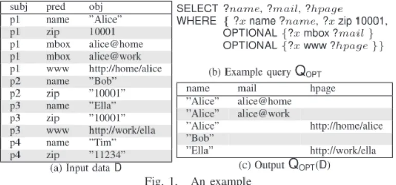
the subgraphs that match any of the n (GP + GPOPT) pattern combinations, plus the results that match just theGP pattern. Consider the data andSPARQLquery in Figure 1(a) and (b). The query looks for triples whose subjects (each corresponding
subj pred obj p1 name ”Alice” p1 zip 10001 p1 mbox alice@home p1 mbox alice@work p1 www http://home/alice p2 name ”Bob” p2 zip ”10001” p3 name ”Ella” p3 zip ”10001” p3 www http://work/ella p4 name ”Tim” p4 zip ”11234”
(a) Input dataD
SELECT ?name,?mail,?hpage
WHERE {?xname ?name,?xzip 10001, OPTIONAL{?xmbox ?mail} OPTIONAL{?xwww ?hpage}} (b) Example queryQOPT
name mail hpage
”Alice” alice@home ”Alice” alice@work ”Alice” http://home/alice ”Bob” ”Ella” http://work/ella (c) OutputQOPT(D) Fig. 1. An example
to a person) have the predicatesnameandzip, with the latter having the value 10001 as object. For these triples, it returns the object of the namepredicate. Due to the firstOPTIONAL
clause, the query also returns the object of predicatembox, if the predicate exists. Due to the secondOPTIONALclause, the query also independently returns the object of predicatewww, if the predicate exists. Evaluating the query over the input data D(can be viewed as a graph) results in output QOPT(D), as shown in Figure 1(c). name zip mbox www ?x ?n 10001 ?m ?p v1 v2 v3 v4 v5 e1 e2 e3 e4
Fig. 2. A query graph We represent queries graphically, and
associate with each query Q (QOPT) a query graph pattern corresponding to its pattern GP (resp., GP (OPTIONAL
GPOPT)+). Formally, a query graph
pat-tern is a 4-tuple (V, E, ν, µ) where V and E stand for vertices and edges, ν and µ are two functions which assign
labels (i.e.,constants and variables) to vertices and edges of
GP respectively. Vertices represent the subjects and objects of a triple; gray vertices represent constants, and white vertices represent variables. Edges represent predicates; dashed edges represent predicates in the optional patternsGPOPT, and solid edges represent predicates in the required patterns GP. Fig-ure 2 shows a pictorial example for the query in FigFig-ure 1(b). Its query graph patterns GP and GPOPTs are defined sepa-rately.GP is defined as (V, E, ν, µ), whereV ={v1, v2, v3}, E ={e1, e2} and the two naming functionsν ={ν1 : v1→
?x, ν2 :v2→?n, ν3 :v3→10001},µ={µ1:e1→name, µ2: e2 → zip}. For the two OPTIONALs, they are defined as
GPOPT1 = (V′, E′, ν′, µ′), where V′ ={v1, v4},E′ ={e3},
ν′ ={ν′
1 : v1→?x, ν2′ : v4→?m}, µ′ ={µ′1 :e3→mbox}; Likewise, GPOPT2 = (V′′, E′′, ν′′, µ′′), whereV′′ ={v1, v5}, E′′ = {e4}, ν′′ = {ν′′
1 : v1 → ?x, ν2′′ : v5 → ?p}, µ′′={µ′′
1 :e4→www}. B. Problem statement
Formally, the problem of MQO in SPARQL, from query rewriting perspective, is defined as follows: Given a data graph
G, and a set Qof Type 1 queries, compute a new setQOPT of
Type 1andType 2queries, evaluateQOPT overGand distribute the results to the queries in Q. There are two requirements for the rewriting approach to MQO: (i) The query results of
QOPT can be used to produce the same results as executing the original queries inQ, which ensures the soundness and com-pletenessof the rewriting; and (ii) the evaluation time ofQOPT,
?z4 ?x4 ?y4 P1 P2 v1 ?z3 ?x3 ?y3 P1 P2 P3 P5 v1 ?z2 ?x2 ?y2 P1 P2 P3 P5 ?w1 v1 ?z1 ?x1 ?y1 P1 P2 P4 P3
(a) QueryQ1 (b) QueryQ2 (c) QueryQ3 (d) QueryQ4
P4 P4 ?w2 ?t2 ?w3 ?u4 P4 ?w4 P3 P6 v1 SELECT* WHERE{?xP1?z,?yP2?z, OPTIONAL{?yP3?w,?wP4v1} OPTIONAL{?tP3?x,?tP5v1,?wP4v1} OPTIONAL{?xP3?y,v1P5?y,?wP4v1} OPTIONAL{?yP3?u,?wP6?u,?wP4v1} } ?z ?x ?y P1 P2 P3 v1 P5 P3 P4 ?t P3 P5 P3 P6 ?w ?u
(e) Example queryQOPT
SELECT* WHERE{?wP4v1, OPTIONAL{?x1P1?z1,?y1P2?z1,?y1P3?w} OPTIONAL{?x2P1?z2,?y2P2?z2,?t2P3?x2,?t2P5v1} OPTIONAL{?x3P1?z3,?y3P2?z3,?x3P3?y3,v1P5?y3} OPTIONAL{?x4P1?z4,?y4P2?z4,?y4P3?u4,?wP6?u4} } pattern p α(p) ?xP1?z 15% ?yP2?z 9% ?yP3?w 18% ?wP4v1 4% ?tP5v1 2% v1P5?t 7% ?wP6?u 13% (f) Structure and cost-based optimization
Fig. 3. Multi-query optimization example
including query rewriting, execution, and result distribution, should be less than the baseline of executing the queries in
Qsequentially. To ease presentation, we assume that the input queries inQare ofType 1, while the output (optimized) queries are either ofType 1orType 2. Our optimization techniques can easily handle more general scenarios where both query types are given as input (section IV).
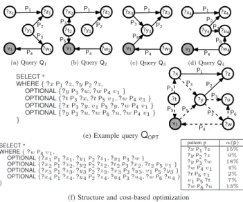
We use a simple example to illustrate the MQOenvisioned and some challenges for the rewriting approach. Figure 3(a)-(d) show the graph representation of four queries of Type 1. Figure 3(e) shows a Type 2 query QOPT that rewrites all four input queries into one. To generate queryQOPT, we identify the (largest) common subquery in all four queries: the subquery involving triples ?xP1?z, ?yP2?z (the second largest
com-mon subquery involves only one predicate, P3 or P4). This
common subquery constitutes the graph pattern GP of QOPT. The remaining subquery of each individual query generates an
OPTIONALclause inQOPT. Note that by generating a query like
QOPT, the triple patterns inGPofQOPTare evaluated onlyonce, instead of being evaluated for multiple times when the input queries are executed independently. Intuitively, this is where the savingsMQOcould bring from. As mentioned earlier,MQO
must consider generic directed graphs, possibly with cyclic patterns, which makes it hard to adapt existing techniques for this optimization. Also, the proposed optimization has a unique characteristic that it leverages SPARQL-specific features such as the OPTIONALclause for query rewriting.
Note that the above rewriting only considers query struc-tures, without considering query selectivity. Suppose we know the selectivityα(p)of each patternpin the queries, as shown in Figure 3(f). Let us assume a simple cost model that the cost of each queryQorQOPTis equal to the minimum selectivity of the patterns in GP; we ignore for now the cost ofOPTIONAL
patterns, which is motivated by how real SPARQL engines evaluate queries (The actual cost model used in this paper is discussed in Section III-D.). So, the cost for all four queries
Q1 toQ4 is respectively4,2,4 and4(with queries executed on a dataset of size 100). Therefore, executing all queries
//J:Jaccard
Input: SetQ={Q1,. . .,Qn} Output: SetQOPTof optimized queries
// Step 1: Bootstrapping the query optimizer
Runk-means onQto generate a setM={M1,. . .,Mk}ofkquery 1
groups based on query similarity in terms of their predicate sets;
// Step 2: Refining query clusters
foreach query groupM∈ Mdo 2
Initialize a setC={C1,. . .,C|M|}of|M|clusters; 3
foreach queryQi∈M,1≤i≤ |M|doCi=Qi; 4
while∃untested pair(Ci,Ci′)withJmax(Ci,Ci′)do 5 LetQii′={Qii′ 1 , . . . ,Qii ′ m}be the queries ofCi∪Ci′; 6
LetSbe the top-smost selective triple patterns inQii′; 7
// Step 2.1: Building compact linegraphs
Letµ∩←µ1∩µ2. . .∩µmandτ={∅}; 8
foreach queryQii′
j ∈ Qii
′ do 9
Build linegraphL(Qii′
j )with only the edges inµ∩; 10
Keep indegree matrixm−
j, outdegree matrixm + j forL(Q ii′ j ); 11
foreach vertexedefined inµ∩andµ∩(e)6=∅do 12 LetI=m−1[e]∩. . .∩m−m[e]andO=m + 1[e]∩. . .∩m+m[e]; 13 ifI=O=∅then µ∩(e) def
=∅andτ=τ∪ {triple pattern one}; 14
forL(GPj),1≤j≤mdo 15
Prune theL(GPj)vertices not inµ∩and their incident edges; 16
// Step 2.2: Building product graphs
BuildL(GPp) =L(GP1)⊗ L(GP2)⊗. . .⊗ L(GPm); 17
// Step 2.3: Finding cliques in product graphs {K1, . . . , Kr}=AllM aximalClique(L(GPp)); 18 ifr= 0then goto22; 19 foreachKi,i= 1,2, . . . , rdo 20 find allK′
i⊆Kihaving the maximal strong covering tree inKi; 21
sortSubQ={K′ 1, . . . , K
′
t} ∪τin descending order by size; 22
InitializeK=∅; 23
foreachqi∈SubQ,i= 1,2, . . . , t+|τ|do 24
ifS ∩qi6=∅thenSetK=qiandbreak 25
ifK6=∅then 26
LetCtmp=Ci∪Ci′andcost(Ctmp)=cost(sub-query forK); 27
ifcost(Ctmp)≤cost(Ci) + cost(Ci′)then 28
PutKwithCtmp; 29
removeCi,Ci′fromCand addCtmp; 30
// Step 3: Generating optimized queries
foreach clusterCiinCdo 31
ifa cliqueKis associated withCithen 32
Rewrite queries inCiusing triple patterns inK; 33
Output the query into setQOPT; 34
returnQOPT. 35
Fig. 4. Multi-query optimization algorithm
individually (without optimization) costs4 + 2 + 4 + 4 = 14. In comparison, the cost of the structure-based only optimized query in Figure 3(e) is9, resulting in a saving of approximately 30%. Now, consider another rewriting in Figure 3(f) that results in from optimization along the second largest common subquery that just containsP4. The cost for this query is only
4, which leads to even more savings, although the rewriting utilizes a smaller common subquery. As this simple example illustrates, it is critical forMQOto construct a cost model that integrates query structure overlap with selectivity estimation.
III. THE ALGORITHM
OurMQOalgorithm, shown in Figure 4, accepts as input a setQ = {Q1,. . .,Qn} ofn queries over a graph G. Without
loss of generality, assume the sets of variables used in different queries are distinct. The algorithm identifies whether there is a cost-effective way to share the evaluation of structurally-overlapping graph patterns among the queries inQ. At a high level, the algorithm works as follows: (1) It partitions the input queries into groups, where queries in the same group are more likely to share common sub-queries that can be optimized through query rewriting; (2) it rewrites a number of Type 1
queries in each group to their correspondent cost-efficient
Type 2 queries; and (3) it executes the rewritten queries and distributesthe query results to the original input queries (along with a refinement). Several challenges arise during the above process: (i) There exists an exponential number of ways to partition the input queries. We thus need a heuristic to prune out the space of less optimal partitioning of queries. (ii) We need an efficient algorithm to identify potential common sub-queries for a given query group. And (iii) since different common sub-queries result in different query rewritings, we need a robust cost model to compare candidate rewriting strategies. We describe how we tackle these challenges next. A. Bootstrapping
Finding structural overlaps for a set of queries amounts to finding the isomorphic subgraphs among the corresponding query graphs. This process is computationally expensive (the problem is NP-hard [4] in general), so ideally we would like to find these overlaps only for groups of queries that will eventually be optimized (rewritten). That is, we want to minimize (or ideally eliminate) the computation spent on identifying common subgraphs for query groups that lead to less optimal MQO solutions. One heuristic we adopt is to quickly prune out subsets of queries that clearly share little in query graphs, without going to the next expensive step of computing their common subqueries; therefore, the group of queries that have few predicates in common will be pruned from further consideration for optimization. We thus define the similarity metric for two queries as the Jaccard similarity of their predicate sets. The rational is that if the Jaccard similarity of two queries is small, their structural overlap in query graphs must also be small; so it is safe to not consider grouping such queries for MQO. We implement this heuristic as a bootstrap step in line 1 using k-means clustering (with Jaccard as the similarity metric) for an initial partitioning of the input queries into a set M of k query groups. Notice that the similarity metric identifies queries with substantial overlaps in their predicate sets, ignoring for now the common sub-structure and the selectivity of these predicates.
B. Refining query clusters
Starting with the k-means generated groups M, we refine the partitioning of queries further based on their structure similarity and the estimated cost. To this end, we consider each query group generated from the k-means clustering M ∈ M
in isolation (since queries across groups are guaranteed to be sufficiently different) and perform the following steps: In lines 5–30, we (incrementally) merge structurally similar queries within M through hierarchical clustering [14], and generate query clusters such that each query cluster is optimized together (i.e.,results in one Type 2query). Initially, we create one singleton cluster Ci for each query Qi of M (line 4).
Given two clustersCi andCi′, we have to determine whether
it is more cost-efficient to merge the two query clusters into a single cluster (i.e.,a singleType 2query) than to keep the two clusters separate (i.e.,executing the corresponding two queries
independently). From the previous iteration, we already know the cost of the optimized queries for each of the Ci and Ci′
clusters. To determine the cost of the merged cluster, we have to compute the query that merges all the queries inCi andCi′
through rewriting; which requires us to compute the common substructure of all these queries, and to estimate the cost of the rewritten query generated from the merged clusters. For the cost computation, we do some preliminary work here (line 7) by identifying the most selective triple patterns from the two clusters (selectivity is estimated by [33]). Note that our refinement ofMmight lead to more than one queries; one for each clusterofM, in the form of eitherType 1 orType 2.
Finding common substructures:While finding the
maxi-mum common subgraph for two graphs is known to be NP-hard [4], the challenge here is asymptotically NP-harder as it requires finding the largest common substructures formultiple graphs. Existing solutions on finding common subgraphs also assumeuntyped edges and nodes inundirected graphs. How-ever, in our case the graphs represent queries, and different triple patterns might correspond to different semantics (i.e., typed and directed). Thus, the predicates and the constants as-sociated with nodes must be taken into consideration. This mix of typed, constant and variable nodes/edges is not typical in classical graph algorithms, and therefore existing solutions can not be directly applied for query optimization. We therefore propose an efficient algorithm to address these challenges.
In a nutshell, our algorithm follows the principle of finding the maximal common edge subgraphs (MCES) [25], [37]. Concisely, three major sub-steps are involved (steps 2.1 to 2.3 in Figure 4): (a) transforming the input query graphs into the equivalent linegraph representations; (b) generating a product graph from the linegraphs; and (c) executing a tailored clique detection algorithm to find the maximal cliques in the product graph (a maximal clique corresponds to an MCES). We describe these sub-steps in details next.
Step 2.1: Building compact linegraphs:The linegraphL(G)
of a graph G is a directed graph built as follows. Each node inL(G)corresponds to an edge inG, and there is an edge be-tween two nodes inL(G)if the corresponding edges inGshare a common node. Although it is straightforward to transform a graph into its linegraph representation, the context ofMQO
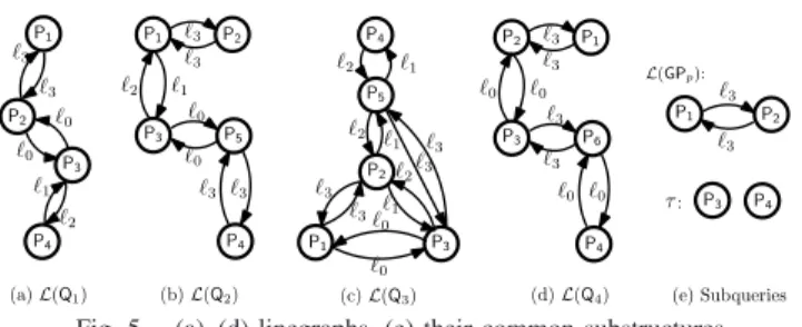
raises new requirements for the linegraph construction. We represent the linegraph of a query graph pattern in a4-tuple, defined asL(G) = (V,E, π, ω). During linegraph construction, besides the inversion of nodes and edges for the query graph, our transformation also assigns to each edge in the linegraph one of4labels (ℓ0 ∼ℓ3). Specifically, for two triple patterns, there are4possible joins between their subjects and objects (ℓ0 = subject-subject, ℓ1 = subject-object, ℓ2 = object-subject, ℓ3 = object-object). The assignment of labels on linegraph edges captures these four join types (useful for pruning and will become clear shortly). Figure 5 (a)-(d) shows the linegraphs for the queries in Figure 3(a)-(d).
The classical solution for finding common substructures of input graphs requires building Cartesian products on their
P2 P1 P3 P4 ℓ3 ℓ3 ℓ0 ℓ0 ℓ1 ℓ2 P5 P1 P3 ℓ3 ℓ3 ℓ3 ℓ0 P2 ℓ3 ℓ1 ℓ2 ℓ1 ℓ2 (a)L(Q1) (b)L(Q2) (c)L(Q3) (d)L(Q4) ℓ0 P2 P1 P3 P5 P4 ℓ3 ℓ3 ℓ2 ℓ1 ℓ0 ℓ0 ℓ3 ℓ3 P4 ℓ2 ℓ1 P1 P2 P3 P6 P4 ℓ3 ℓ3 ℓ0 ℓ0 ℓ3 ℓ3 ℓ0 ℓ0 (e) Subqueries ℓ3 ℓ3 P2 P1 L(GPp): τ: P3 P4
Fig. 5. (a)–(d) linegraphs, (e) their common substructures
linegraphs. This raises challenges in scalability when finding the maximum common substructure for multiple queries in one shot. To avoid the foreseeable explosion, we propose fine-grained optimizations (lines 8–16) to keep linegraphs as small as possible so that only the mostpromisingsubstructures would be transformed into linegraphs, with the rest being temporarilymasked from further processing.
To achieve the above, queries in Qii′ pass through a two-stage optimization. In the first stage (lines 8–11), we identify (line 8) the common predicates in Qii′ by building
the intersectionµ∩ for all the labels defined in theµ’s (recall
that function µ assigns predicate names to graph edges). Predicates that are not common to all queries can be safely pruned, since by definition they are not part of any common substructure, e.g.,P5 and P6 in Figure 3. While computing
the intersection of predicates, the algorithm also checks for compatibilitybetween the corresponding subjects and objects, so that same-label predicates with different subjects/objects are not added intoµ∩. In addition, we maintain two adjacency
matrices for a linegraph L(GP), namely, the indegree matrix m−storing all incoming, and the outdegree matrixm+storing all outgoing edges fromL(GP)vertices. For a vertexv, we use m−[v] andm+[v], respectively, to denote the portion of the adjacency matrices storing the incoming and outgoing edges of v. For example, the adjacency matrices for vertex P3 in
linegraph L(Q1)of Figure 5 are m+1[P3] = [∅, ℓ0,∅, ℓ2,∅,∅],
m−1[P3] = [∅, ℓ0,∅, ℓ1,∅,∅], while for linegraph L(Q2) they
are m+2[P3] = [ℓ2,∅,∅,∅, ℓ0,∅],m−2[P3] = [ℓ1,∅,∅,∅, ℓ0,∅].
In the second stage (lines12–16), to further reduce the size of linegraphs, for each linegraph vertex e, we compute the Boolean intersection for the m−[e]’s and m+[e]’s from all linegraphs respectively (line 13). We also prune e from µ∩
if both intersections equal ∅ and set aside the triple pattern associated withein a setτ (line14). Intuitively, this optimiza-tion acts as a look-ahead step in our algorithm, as it quickly detects the cases where the common sub-queries involve only one triple pattern (those in τ). Moreover, it also improves the efficiency of the clique detection (step 2.2 and 2.3) due to the smaller sizes of input linegraphs. Going back to our example, just by looking at them−1,m+1,m−2,m+2, it is easy to see that the intersection ∩m+i [P3] =∩m−i [P3] =∅ for all
the linegraphs of Figure 5(a)-(d). Therefore, our optimization temporarily masks P3 (so as P4) from the expensive clique
detection in the following two steps.
Step 2.2: Building product graphs: The product graph
L(GPp) := (Vp,Ep, πp, ωp) of two linegraphs, L(GP1) :=
(V1,E1, π1, ω1)andL(GP2) := (V2,E2, π2, ω2), is denoted as
L(GPp) := L(GP1)⊗ L(GP2). The vertices Vp in L(GPp)
are defined on the Cartesian product of V1 and V2. In order to use product graphs in MQO, we optimize the standard definition with the additional requirement that vertices paired together must have the same label (i.e., predicate). That is,
Vp := {(v1, v2) | v1 ∈ V1∧v2 ∈ V2∧π1(v1) = π2(v2)}, with the labeling function defined asπp:={πp(v)|πp(v) =
π1(v1), withv = (v1, v2)∈ Vp}. For the product edges, we
use the standard definition which creates edges in the product graph between two vertices (v1i, v2i) and(v1j, v2j) inVp if
either (i) the same edges(v1i, v1j)inE1, and(v2i, v2j)inE2 exist; or (ii) no edges connect v1i with v1j in E1, and v2i
with v2j in E2. The edges due to (i) are termed as strong
connections, while those for (ii) asweak connections [37]. Since the product graph for two linegraphs conforms to the definition of linegraph, we can recursively build the product for multiple linegraphs (line 17). Theoretically, there is an exponential blowup in size when we construct the product for multiple linegraphs. In practice, thanks to our optimizations in Steps 2.1 and 2.2, our algorithm is able to accommodate tens to hundred of queries, and generates the product graph efficiently (which will be verified through Section V). Figure 5(e) shows the product linegraphL(GPp)for the running example.
Step 2.3: Finding Cliques in product graphs:A (maximal)
clique with a strong covering tree (a tree only involving strong connections) in the product graph equals to an MCES – a (maximal) common sub-query in essence. In addition, we are interested in finding cost-effective common sub-queries. To verify if the found common sub-query is selective, it is checked with the setS(from line7) of selective query patterns. In the algorithm, we proceed by finding all maximal cliques in the product graph (line 18), a process for which many efficient algorithms exist [16], [21], [35]. For each discovered clique, we identify its sub-cliques with the maximal strong covering trees (line 21). For the L(GPp) in Figure 5(e), it results in one clique (itself):i.e.,K′
1={P1,P2}. As the cost
of sub-queries is another dimension for query optimization, we look for the substructures that are both large in size (i.e.,the number of query graph patterns in overlap) and correspond to selective common sub-queries. Therefore, we first sort SubQ
(contributed byK′s andτ, line22) by their sizes in descending order, and then loop through the sorted list from the beginning and stop at thefirst substructure that intersects S (lines 22– 25), i.e., P4 in our example. We then merge (if it is
cost-effective, line 28) the queries whose common sub-query is reflected in K and also merge their corresponding clusters into a new cluster (while remembering the found common sub-query) (lines 26–30). The algorithm repeats lines 5–30 until every possible pair of clusters have been tested and no new cluster can be generated.
C. Generating optimized queries and distributing results After the clusters are finalized, the algorithm rewrites each cluster of queries into one query and thus generates a set of rewritingsQOPT(lines31–34). The result from evaluatingQOPT
(more expositions in section III-E). Therefore, we must filter and distribute the results from the execution of QOPT. This necessitates one more step of parsing the result of QOPT (refer to Figure 1(c)), which checks each row of the result against the RD of each query in Q. Note that the result description
RDOPT is always the union of RDis from the queries being
optimized, and we record the mappings between the variables in the rewritings and the variables in the original input queries. As in Figure 1(c), the result of a Type 2 query might have empty(null) columns corresponding to the variables from the
OPTIONAL clause. Therefore, a row in the result of RDOPT
might not conform to the description of every RDi. The
goal of parsing is to identify the valid overlap between each row of the result and the individual RDi, and return to each
query the result it is supposed to get. To achieve this, the parsing algorithm performs a Boolean intersection between each row of result and each RDi: if the columns of this
row corresponding to those columns of RDi are not null, the
algorithm distributes the corresponding part of this row to Qi
as one of its query answers. This step iterates over each row and each Qi that composed the Type 2 query. The parsing on
the results of QOPT only requires a linear scan on the results to the rewritten query. Therefore, it can be done on-the-fly as the results of QOPT is streamed out from the evaluation. D. Cost model for SPARQL MQO
The design of our cost module is motivated by the way in which a SPARQL query is evaluated on popular RDFstores. This includes a well-justified principle that the most selective triple pattern is evaluated first [33] and that the GPOPT clause is evaluated on the result of GP (for the fact that GPOPT is a left-join). This suggests that a good optimization should keep the result cardinality from the common sub-query as small as possible for two reasons:1) The result cardinality of aType 2
SPARQL query is upper bounded by result cardinality of its
GP clause since GPOPTs are simply left-joins; 2) Intermediate result from evaluating theGPclause is not well indexed, which implies that a non-selectiveGPwill result in significantly more efforts in processing the corresponding rewriting GPOPTs.
In [33], the authors discussed the selectivity estimation for the conjunctive Basic Graph Patterns (BGP). In a nut-shell, given a triple pattern t = (s p o), where each entry could be bound or unbound, its selectivity is estimated by sel(t) = sel(s) × sel(p) ×sel(o). sel is the selectivity estimation function, whose value falls in the interval of[0,1]. Specifically, for unbound variable, its selectivity equals 1. For bound variables/constants, depending on whether it is a subject, predicate or object, different methods (e.g., [33]) are used to implement sel. Notice that the formula implicitly assumes statistical independence for the subject, predicate and object; thus is an approximation. Pre-computed statistics of the dataset are also required. For a join between two triple patterns, independence assumption is adopted [33]. However, in practice, such estimation is not accurate enough for op-timizing complex queries. The culprit comes from the fact that as the number of joins increases, the accuracy of the
estimated selectivity drops quickly, resulting in a very loose estimation [19].
With the above limitations in mind, we propose a cost function for conjunctiveSPARQLquery. It has a simple design and roots on the well justified principle in query optimization that the selective triple patterns have higher priorities in evaluation. Our cost model is an incarnation of this intuition, as in Formula 1:
Cost(Q) =
(
Min(sel(t)) Qis aType 1query,t∈GP Min(sel(t)) + ∆ Qis aType 2query,t∈GP
(1) For a Type 1 conjunctive query, Formula 1 simply returns the selectivity for the most selective triple pattern in the query graph GP as the cost of evaluating Q. For a Type 2
query, the cost is the summation of the cost on evaluating the common graph patternGP and the cost on the evaluating
the OPTIONALs, i.e., the cost denoted by ∆. We
extrapo-late (backed by a comprehensive empirical study on three different RDF query engines) that ∆ is a hidden function of (i) the cost of GP; (ii) the number of OPTIONALs; and (iii) the cost of the query pattern of each GPOPT. However, we observed empirically that when the cost of GP is small (being selective), ∆ would be a trivial value and Cost(Q) is mostly credited to the evaluation of GP. Hence, we can approximateCost(Q) with the cost of GP in such cases. We show (experimentally) that using our cost model to choose a good common substructure can consistently improve the performance of query evaluation over the pure structure-based optimization (i.e.,without considering the evaluation cost of common sub-queries) on differentRDFstores.
Finally, notice that the proposed cost function requires using the pre-computed statistics of theRDFdataset to estimate the selectivity of triple patterns. Therefore, it requires to collect some statistics from the dataset. This mainly includes (i) building the histogram for distinct predicates in the dataset and (ii) that for each disparate predicate, we build histograms for the subjects and objects attached to this predicate in the dataset. In practice, for some RDF stores, like Jena, part of such statistics (e.g., the histogram of predicates) is provided by the SPARQL query optimizer and is accessible for free; for the others,e.g.,Virtuoso and Sesame, the statistics of the dataset need to be collected in a preprocessing step.
E. Completeness and soundness of our MQO algorithm
Completeness: Suppose a Type 2 rewritten query QOPT
opti-mizes a set ofn Type 1 queries, i.e.,Q={Q1,Q2, . . . ,Qn}.
Without loss of generality, denote the common relation (i.e., the common sub-query) used in QOPT as GP and its outer join relations (i.e.,theOPTIONALs) asGPi (i= 1,2, . . . , n).
As we only consider conjunctive queries as input, hence by constructionQ=∪n
i=1GP⋊⋉GPiandQOPT=∪ni=1GP GPi.
By the definition of left outer join ,GP ⋊⋉ GPi⊆GP GPi
for anyi. It followsQ ⊆QOPT in terms of query results.
Soundness:Soundness requiresQ ⊇QOPT. This is achieved by
results to correspondent queries inQ(section III-C). As such, false positives are discarded and the remainings are valid bindings for one or more graph patterns in Q. Therefore,
Q ⊇QOPT in terms of results after the refining step.
Completeness and soundness together guarantee that the final answers resulted by our MQOtechniques are equivalent to the results from evaluating queries inQ independently.
IV. EXTENSIONS
For the ease of presentation, the input queries discussed so far areType 1queries using constants as their predicates. It is interesting to note that with some minimal modifications to the algorithm and little preprocessing of the input, the algorithm in Figure 4 can optimize more general SPARQL queries. Here, we introduce two simple yet useful extensions: (i) optimizing input queries with variables as the predicates; and (ii) optimizing input queries ofType 2(i.e.,withOPTIONALs). A. Queries with variable predicates
We treat variable predicates slightly differently from the constant predicates when identifying the structural overlap of input queries. Basically, a variable predicate from one query can be matched with any variable predicate in another query. In addition, each variable predicate of a query will correspond to one variable vertex in the linegraph representation, but the main flow of the MQO algorithm remains the same.
B. TYPE 2 queries
Our MQO algorithm takes a batch of Type 1 SPARQL
queries as input and rewrites them to another batch of Type 1
andType 2 queries. It can be extended to optimize a batch of input queries with bothType 1 andType 2queries.
To this end, it requires a preprocessing step on the input queries. Specifically, by the definition of left-join, a Type 2
input query will be rewritten into its equivalent Type 1 form, since our MQO algorithm only works onType 1input queries. The equivalent Type 1form of aType 2queryGP(OPTIONAL
GPOPT)+) consists two sets of queries: (i) aType 1query solely
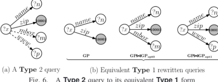
using the GP as its query graph pattern; and (ii) the queries by replacing the left join(s) with inner join(s) betweenGPand each of the GPOPT from the OPTIONAL, i.e., ∪GP ⋊⋉ GPOPT. For example, to strip off the OPTIONALs in theType 2 query in Figure 6(a), applying the above preprocessing will result in a group of threeType 1 rewritings as in Figure 6(b).
name zip mbox www ?x ?n 10001 ?m ?p name zip ?x ?n 10001 name zip mbox ?x ?n 10001 ?m name zip www ?x ?n 10001 ?p
(a) AType2 query (b) EquivalentType1 rewritten queries
GP GP GPopt0 GP GPopt1
| {z }
Fig. 6. AType 2query to its equivalentType 1form
By applying the above transformation to all Type 2 queries in the input and then passing the batch of queries to algorithm in Figure 4 for optimization, we can handle Type 2 queries seamlessly. Finally, the result to the original Type 2 query
can be generated through the union of the results, from the transformedType 1 queries afterMQO.
V. EXPERIMENTALEVALUATION 1 5 10 15 20 25 30 35 40 45 50 10−1 100 101 Selectivity (%) Predicate ID Selective Non−selective
Fig. 7. Predicate selectivity We implemented all algorithms in
C++ and performed an extensive ex-perimental evaluation using a64-bit Linux machine with a 2GHz Intel Xeon(R) CPU and4GB of memory.
Datasets: Our evaluation is based
on LUBM benchmark. The popular benchmark models universities with
students, departments,etc., using only18predicates [11]. This limits the complexity of queries we can evaluate (similar lim-itations in [5], [28]), and results in queries with considerable overlaps (which favors MQO but is not very realistic). Thus, we extended the LUBM data generator, and added a random subset from 50new predicates to each person in the dataset, where predicate selectivity follows the distribution in Figure 7. Therefore, given the number of triples N in a dataset D, the number of times that a predicate appears in D (dubbed its frequency) is precisely its selectivity multiplied by N.
RDF Stores:We experimented with three popularRDFstores:
Jena TDB0.85, OpenLink Virtuoso6.01, and Sesame Native 2.0. Due to space constraints, we analyze mainly the exper-iments with Jena TDB. Results for the other two stores are highly consistent with the results from Jena TDB. For all stores, we created full indexes using the technique in [39]. For Virtuoso, we also built bitmap indexes as reported in [3].
Metrics: For all experiments, we measure the number of
optimized queries and their end-to-end evaluation time, in-cluding query rewriting, execution and result distribution. We compare ourMQOalgorithm with the evaluation without any optimization (i.e.,No-MQO), and the approach with structure-only optimization (i.e.,MQO-S). To realize the latter strategy as a baseline solution, we need to turn off all the cost-based comparisons in Figure 4. Specifically, in line 24of Figure 4, instead of walking through the set ofSubQ(which correspond to different common substructures), structure-based optimiza-tion (i.e., MQO-S) simply returns the the largest clique (i.e., the largest common subquery) for optimization.
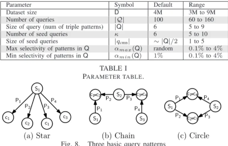
Comparing MQO with MQO-S illustrates the benefits of blending structured-based with the cost-based optimization versus a purely structural approach. In the algorithms, we use the suffix -C to denote the cost by rewriting queries (e.g.,MQO-C) and the suffix-Pto denote the cost by parsing and distributing the query results (e.g., MQO-P). For finding cliques, we customized the Cliquer library [21], which is an efficient implementations for clique detection. For selectivity estimation, we implemented the technique in [33]. All experi-ments are performed using cold caches, and the bootstrapping parameterkin thek-means algorithm is set tok=⌈|Q|/40⌉. Table I provides the summary along with ranges and the default values used for various parameters in our experiments.
Queries:LUBMhas only 14SPARQLqueries, which have
Parameter Symbol Default Range
Dataset size D 4M 3M to 9M
Number of queries |Q| 100 60 to 160
Size of query (num of triple patterns) |Q| 6 5 to 9
Number of seed queries κ 6 5 to 10
Size of seed queries |qcmn| ∼ |Q|/2 1 to 5 Max selectivity of patterns inQ αmax(Q) random 0.1%to4%
Min selectivity of patterns inQ αmin(Q) 1% 0.1%to4% TABLE I PARAMETER TABLE. S1 S1 S3 S2 S1 S2 P1 P2 P3 P4 c1 c2 c1 c3 P1 P2 P3 P4 P1 P2 P3 P4 c1c2 c3c4 c1c4 c2c3
(a) Star (b) Chain (c) Circle
Fig. 8. Three basic query patterns
we created a module to generate query sets Q with varying sizes|Q|, where we generated queries that combinestar,chain, andcircle pattern structures. In addition, we attached to each person (as a subject) in the LUBM data a (random) subset of 50 new predicates P1 ∼ P50. In particular, we customized
the data generator of LUBM in such a way that whenever a triple (s Pici) is added to the data, ci is an integer value
serving as the object of this triple and it is set to the number of predicatePiexisted in the dataset so far. Therefore, triples
with different predicates could join on their subjects or objects, so as the triple patterns in the query, which we will detail next. Our query generator utilizes the aforementioned patterns in the customized data to compose queries. Specifically, we ensure that the queries have reasonably high randomness in structure (such that they are not replicas of limited query templates) and reasonable variances in selectivity (such that any predicate could be part of a query regardless of the structure). To this end, we first show how to compose three basic query patterns: star, chain and circle with a set of four basic triple patterns; see Figure 8 (a) – (c). The star and the chain can be built with any number of triple patterns while the circle can only be built with an even number of triple patterns. To blend the three basic patterns into one query Q with
|Q| triple patterns, the generator first randomly distributes the set of triple patterns into k groups of subqueries (k is a random integer, k∈(0,|Q|)), with each subquery randomly composing one of the three basic patterns, i.e., star, chain and if possible, circle. To ensure Q to be conjunctive, the generator then makes equal the (randomly) chosen pairs of subjects and/or objects from theksubqueries by unifying their variable names or binding them to the same constant. This concludes composing the structure ofQ. Finally, to ensure that
Qconforms to the selectivity requirement posed by a specific experiment (refer to Table I), the generator fills in the structure ofQwith the predicates that would makeQa legitimate query. In the experiments, a group of queries in Qwere rendered to share a common seed sub-query qcmn. The generator first
constructs qcmn and the remaining portion of the queries
independently. Then, by equaling the subjects and/or objects of these two sub-queries, the generator propagates qcmn over
the group such that qcmn joins with each of the sub-queries
in the group. In addition, individual query sizes |Q| can be
varied where the probability of a predicate being part of a query conforms to its frequency in the dataset. We ensure that 90% of the queries inQ are amenable to optimization, while 10%are not. We use a parameterκto determine seed queries that will be used to generate the queries in this 90%. For a givenκ,κ seed-groups are generated, each corresponding to
⌈(90/κ)⌉% of queries in Q. The seed in each seed-group is what our algorithm will (hopefully) discover.
In short, we generated datasets and queries with various size, complexity, and statistics to evaluate the proposedMQO algorithm in a comprehensive way.
A. Experimental Results
The objective of our experiments is to evaluate: (i) how much each step of MQO (from bootstrapping step to cost estimation) contributes to the optimization,i.e.,drop in perfor-mance due to omission of each step; (ii) whether the combi-nation of structure and cost-based optimization consistently outperforms purely structure-based optimizations; (iii) how well Algorithm MQOoptimizes its alternatives, including the comparison with the baseline approach without any optimiza-tion, ineveryexperimental setting; and (iv) whether Algorithm MQOconsistently works acrossRDFstores.
60 80 100 120 140 160 100 101 Time (seconds) MQO−noKM−C MQO−C |Q|
Fig. 9. Clustering time
100 101 102 200 220 240 260 Time (seconds) No−MQO MQO−KM
Number ofk-means clusters
Fig. 10. Evaluation time
Impact of each MQO step:We start with an experiment to
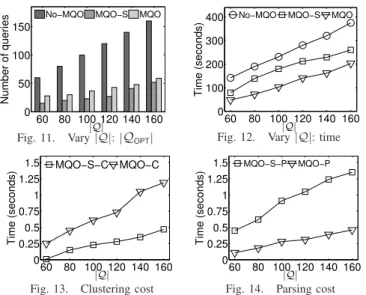
illustrate the benefit of bootstrapping MQO using k-means. Figure 9 shows the cost of hierarchical clustering in Step 2 of MQO with (MQO-C) and without (MQO-noKM-C) boot-strapping. The figure shows an order of magnitude difference between the MQO-C and MQO-noKM-C, since without boot-strapping Step 2 of MQO requires O((|Q| × |Q|)2) pairwise checks between all the queries in the input set Q. The next experiment, in Figure 10, illustrates algorithmMQO-KMwhich after Step 1 ofMQO, it finds the common substructures for the coarse-grained groups that result in from k-means and then performs Step 3 (i.e.,MQO-KMdoes not perform hierarchical clustering in Step 2). The figure shows that the resulting optimization has limited (less than 10%) to no benefits in evaluation time, when compared with the case of having no optimizations (No-MQO). This is because k-means ignores query structures and relies solely on the predicate names to determine groups. Therefore, the fine-grained groups that result in from hierarchical clustering (in Step 2) arenecessary for the considerable savings (as illustrated in the following experiments) in terms of evaluation times.
Varying|Q|:We study scalability w.r.t. the cardinality|Q|of
the query set Q, for which we vary from 60 to160 queries, by an increment of 20. As Figure 11 shows, both MQO and MQO-S are successful in identifying common substructures,
60 80 100 120 140 160 0 50 100 150 Number of queries
No−MQO MQO−S MQO
|Q|
Fig. 11. Vary|Q|:|QOPT|
60 80 100 120 140 160 0 100 200 300 400 Time (seconds)
No−MQO MQO−S MQO
|Q|
Fig. 12. Vary|Q|: time
60 80 100 120 140 160 0 0.25 0.5 0.75 1 1.25 1.5 Time (seconds) MQO−S−C MQO−C |Q|
Fig. 13. Clustering cost
60 80 100 120 140 160 0 0.25 0.5 0.75 1 1.25 1.5 Time (seconds) MQO−S−P MQO−P |Q|
Fig. 14. Parsing cost
the former resulting in up to 60% savings and the latter having up to 80% savings in terms of the number of queries, compared toNo-MQO. However, in terms of evaluation times (see Figure 12), MQO-S results in less savings than MQO, with the former achieving up to 45%, and the latter up to 60%savings in evaluation times, when compared toNo-MQO. SoMQOis more efficient, despite generating a larger number of optimized queries than MQO-S. The following example, along with the example in Figure 3, illustrates this situation. Consider a set of queries Q, such that (i) predicate pcmn is
common to all the queries inQ; (ii) predicatep1 is common to the subsetQ1⊂ Q; and (iii) predicatep2 is common to the subset of queries inQ2⊂ Q, withQ1∩Q2=∅.MQO-Slooks only at the structure and thus it may opt to generate a single optimized query for Q withqcmn=pcmn. If predicate pcmn is
not selective, while predicatesp1 andp2 are highly selective, then MQOwill generate two different optimized queries, one for setQ1and involvingq1, and one for setQ2 and involving p2. As this simple example illustrates, MQO-S can generate fewer but cost-wise less optimized queries when compared withMQO; which is exactly the pattern in Figure 12.
Next, we further analyze the evaluating cost spent on clus-tering/rewriting the queries, and distributing the final results. In Figure 13, we report the clustering time, which includes both the bootstrappingk-means clustering and the hierarchical clustering that relies on finding common substructures. Notice thatMQOrequires more time thanMQO-S. This is because (i) MQO involves an additional check on the selectivity; and (ii) queries with non-selective common subqueries are recycled into the pool of clusters by MQO, leading to more rounds of comparisons and thus a slower convergence. Contrarily, since the common subqueries rewritten by MQO-S are on average less selective, parsing and distributing these results inevitably requires more effort, as in Figure 14. Nevertheless, clustering and parsing times are a small fraction of the total evaluating cost (less than 2% in the worst case). In the remaining experiments, we only report the end-to-end evaluating cost.
Varying|qcmn|:Here, we study the impact on optimization of
the size |qcmn| of the common subquery, i.e., the size of seed
1 2 3 4 5 0 25 50 75 100 Number of queries
No−MQO MQO−S MQO
|qcmn|
Fig. 15. Vary|qcmn|:|QOPT|
1 2 3 4 5 0 100 200 300 400 Time (seconds)
No−MQO MQO−S MQO
|qcmn|
Fig. 16. Vary|qcmn|: time
queries. At iteration i we make sure that for the queries in the same group of Q, we have |qcmn| = i. Figure 15 shows
the number of optimized queries generated by MQO-S and MQO. Notice that the number of optimized queries is reduced (optimization improves) as|qcmn| increases . This is because,
as the maximum size of each query is kept constant, the more|qcmn|increases the more the generated queries become
similar (less randomness in query generation). Therefore, more queries are clustered and optimized together. Like before, MQO-Sis more aggressive and results in less queries compared toMQO. But, like before, Figure 16 shows thatMQOisalways better and results in optimized queries whose evaluation time is half less thanMQO-Sand up to75%less thanNo-MQO. Notice in the figure that for small values of|qcmn|,MQO-Sperforms
worse thanNo-MQO. Intuitively, the more selectiveGPis in a
Type 2optimized query, the lessworkaSPARQLquery engine needs to do to evaluate theGPOPT terms in theOPTIONALof
the query.MQO-Srelies only on the structural similarity, while ignoring predicate selectivity, negatively influences the overall evaluation time for the optimized query to the point that any benefits from the optimization are alleviated by the extra cost of evaluating theOPTIONALterms.
1 2 3 4 5 60 80 100 Percentage (%) MQO−S MQO |qcmn| No−OPTIONAL − − − Fig. 17.Evaluatingqcmn
MQO combines structured and cost optimization and does not suffer from these limitations. This is evident in Figure 17, which plots the percentage of the evalu-ation time of the optimized query that is spent evaluating qcmn. By
carefully selecting the common subqueryqcmn,MQOresults in
optimized queries whose evaluation time goes mostly (more than 90%) into evaluating qcmn (while less than 10% goes
to evaluating OPTIONAL terms). In contrast, MQO-S results in queries whose large extent of evaluation time goes into evaluating OPTIONAL terms (when |qcmn| = 1this is almost
30%). Things improve forMQO-Sas the size ofqcmnincreases,
but stillMQOretains the advantage of selecting substructures not just based on their size, but also on their selectivity, and therefore overall evaluation times are still much better.
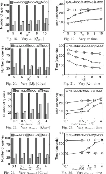
Varyingκ:In Figures 18 and 19, we analyze the impact of the
numberκ of seed queries on the optimization, by varying κ from5to10. Figure 18 shows that asκincreases, less queries can be optimized by bothMQO-SandMQO, which resulted in more rewritten queries. Not surprisingly, a larger κincreases query diversity and reduces the potential for optimization. This affects evaluation times, butMQOis still the best of the three.
5 6 7 8 10 0 25 50 75 100 Number of queries
No−MQO MQO−S MQO
κ
Fig. 18. Varyκ:|QOPT|
5 6 7 8 9 10 0 100 200 300 Time (seconds)
No−MQO MQO−S MQO
κ Fig. 19. Varyκ: time
5 6 7 8 9 0 25 50 75 100 Number of queries
No−MQO MQO−S MQO
|Q|
Fig. 20. Vary|Q|:|QOPT|
5 6 7 8 9 0 100 200 300 Time (seconds)
No−MQO MQO−S MQO
|Q|
Fig. 21. Vary|Q|: time
0.1 0.5 1 2 4 0 25 50 75 100 Number of queries
No−MQO MQO−S MQO
αmin(qcmn) (%)
Fig. 22. Varyαmin:|QOPT|
0.1 0.5 1 2 4 0 100 200 300 Time (seconds)
No−MQO MQO−S MQO
αmin(qcmn) (%)
Fig. 23. Varyαmin: time
0.1 0.5 1 2 4 0 25 50 75 100 Number of queries
No−MQO MQO−S MQO
αmax(Q) (%)
Fig. 24. Varyαmax:|QOPT|
0.1 0.5 1 2 4 0 100 200 300 Time (seconds)
No−MQO MQO−S MQO
αmax(Q) (%)
Fig. 25. Varyαmax: time
query size, which we increase from5to9predicates inGPof a queryQ. For this experiment wekeep the|qcmn|/|Q|a rough
constant and equal to 0.5. So, the increase in query size does not result in a significant change in query overlap (or potential for optimization). Since the size of a query increases, there is higher chance for the query generator to assign it a selective predicate, which in turn affects the evaluation times. As a result, Figure 21 shows that the evaluation time of No-MQO decreases with the query size. Clearly, MQO still provides savings in evaluation time, ranging from40% to70%.
Varying αmin(qcmn): We study the impact of the
mini-mum predicate selectivity in qcmn (seed query), by varying
αmin(qcmn)from0.1%to4%. As Figure 22 shows, selectivity
has minimal impact forMQO-Swhich ignores evaluation costs, but noticeable impact in MQO. As selectivity is reduced, the number of optimized queries increases (less optimization) sinceMQOincreasingly rejects optimizations that lead to more expensive (non-selective) common subqueries. While reduced selectivity increases the evaluation time of queries for all algorithms (Figure 23),MQO still achieves between10%and 50% savings in evaluation times.
Varying αmax(Q):While changing minimum selectivity has
an impact on deciding the sub-structure that forms qcmn,
maximum selectivity mostly affects the cost of evaluating the (non-seed) OPTIONAL terms. Here, we vary the maximum selectivity for predicates in a query, αmax(Q), from 0.1%
to 4%. Like before, Figure 24 shows that the number of optimized queries is almost unaffected for MQO-S. Unlike the previous experiment, this number is also unaffected for algorithm MQO since the change in selectivity concerns OPTIONAL predicates and thus has less of an effect in the generation of optimized queries. Figure 25 shows that both MQO-SandMQO outperformNo-MQO, with MQOachieving aminimumof 50% savings. Again, notice that whenMQO-S chooses non-selective predicates for optimization, evaluation times quickly degrade toNo-MQOas whenαmax(Q)>1%.
2 4 6 8 10
0 100 200 300
Data size (× 106 triples)
Time (seconds)
No−MQO MQO−S MQO
Fig. 26. Varying|D|
Varying |D|: We investigate the
impact of dataset size |D| on the optimization results, by varying|D|
from 3M to 9M triples. While this does not affect the number of rewritings of Q it clearly affects evaluation times, as shown in Fig-ures 26. Notice that MQO
consis-tently has aminimumof 50%(achieving up to 65%) savings.
Effect of our cost model:In Section III, we extrapolate that
the evaluation cost of a Type 2 query is inversely correlated with the estimated cost of GP, i.e., the minimum selectivity of its triple patterns. This is indeed a reasonable approxima-tion in practice. As shown in Figure 23, reduced minimum selectivity in the common subquery GP would incur higher evaluation cost forType 2queries. Similarly, both the number ofOPTIONALs and the cost of the query pattern of eachGPOPT
are indispensable factors in determining the value of ∆, as shown respectively in Figure 19 and Figure 16. However, we observed that when the cost ofGP is small (being selective), ∆ would be a trivial value and Cost(Q) is mostly credited to the evaluation of GP. This is clearly shown in Figure 17 that whenGPis selective, the dominant cost is contributed by evaluating GP (more than 90%) with the rest factors being almost irrelevant. This suggests that when dealing with a selectiveGP, a possibly good approximation of Cost(Q) can set ∆ ≃ 0. This observation also motivates us to choose a selectiveGP in rewriting. In practice, this simple cost model and its approximation give excellent cost estimation inMQO.
Results from other stores: Up to now, all results reported
were performed with Jena TDB. Using the same queries and parameters, we also ran the experiments on Virtuoso and Sesame native, to evaluate the desired property of store inde-pendence. In general, the results from Virtuoso and Sesame are consistent with what we observed in Jena TDB, see Figures 27∼32 when we used the same setup as that in the experiments for Jena TDB, and varied values of one parameter while using default values for all other parameters. The proposed optimization algorithm, MQO, significantly reduces the evaluation time of multipleSPARQLqueries on both stores.
60 80 100 120 140 160 0 30 60 90 120 150 Time (seconds)
No−MQO MQO−S MQO
|Q| (a) Virtuoso 60 80 100 120 140 160 0 40 80 120 160 200 Time (seconds)
No−MQO MQO−S MQO
|Q|
(b) Sesame Fig. 27. Vary|Q|: evaluation time
0.1 0.5 1 2 4 0 30 60 90 120 150 Time (seconds)
No−MQO MQO−S MQO
αmin(qcmn) (%) (a) Virtuoso 0.1 0.5 1 2 4 0 50 100 150 200 Time (seconds)
No−MQO MQO−S MQO
αmin(qcmn) (%)
(b) Sesame Fig. 28. Varyαmin(qcmn): evaluation time
0.1 0.5 1 2 4 0 50 100 150 Time (seconds)
No−MQO MQO−S MQO
αmax(Q) (%) (a) Virtuoso 0.1 0.5 1 2 4 0 50 100 150 200 Time (seconds)
No−MQO MQO−S MQO
αmax(Q) (%)
(b) Sesame Fig. 29. Varyαmax(Q): evaluation time
In particular, we consistently observed that the cost-based op-timization can remarkably improve the performance in almost all experiments, leading to a 40%–75%speedup compared to No-MQO on both Virtuoso and Sesame. For example, using the same setting and optimized queries as Figure 12 where we vary the number of queries in a batch Q, Figures 27(a) and 27(b) report the results from Virtuoso and Sesame. It is clear that MQO consistently outperforms MQO-S and No-MQO, leading to savings of 50%–60% across engines. Similarly, in the experiment that studies the impact of minimum selectivity in qcmn, i.e., Figure 28(a) and Figure 28(b), reducing the
minimum selectivity of qcmn results in increasing evaluation
times for all algorithms. While MQO-S is sensitive to such variance since it does not proactively take cost into account, MQO still achieves 40%–75% savings in evaluation times.
VI. RELATEDWORK
The problem of multi-query optimization has been well studied in relational databases [22], [27], [31], [32], [42]. The main idea is to identify the common sub-expressions in a batch of queries. Global optimized query plans are constructed by reordering the join sequences and sharing the intermediate results within the same group of queries, therefore minimizing the cost for evaluating the common sub-expressions. The same principle was also applied in [27], which proposed a set of heuristics based on dynamic programming to deal with nested sub-expressions. There has also been studies on identifying common expressions [10], [40] with complexity analysis of
1 2 3 4 5 0 50 100 150 Time (seconds)
No−MQO MQO−S MQO
|qcmn| (a) Virtuoso 1 2 3 4 5 0 50 100 150 200 Time (seconds)
No−MQO MQO−S MQO
|qcmn|
(b) Sesame Fig. 30. Vary|qcmn|: evaluation time
5 6 7 8 9 0 50 100 Time (seconds)
No−MQO MQO−S MQO
|Q| (a) Virtuoso 5 6 7 8 9 0 50 100 150 200 Time (seconds)
No−MQO MQO−S MQO
|Q|
(b) Sesame Fig. 31. Vary|Q|: evaluation time
5 6 7 8 9 10 0 25 50 75 100 Time (seconds)
No−MQO MQO−S MQO
κ (a) Virtuoso 5 6 7 8 9 10 0 50 100 150 200 Time (seconds)
No−MQO MQO−S MQO
κ (b) Sesame Fig. 32. Varyκ: evaluation time
MQO; the general MQO problem for relational databases is NP-hard. Even with heuristics, the search space for individual candidate plans and their combinatorial hybrid (i.e.,the global plan) is often astronomical [27]. In light of the hardness, [27] proposed some heuristics which were shown to work well in practice; however, those heuristics were proposed to work inside query optimizers (i.e.,engine dependent), and are only applicable when the query plans are expressible as AND-OR DAGs. Dalvi et al. [7] considered pipelining intermediate results to avoid unnecessary materialization. In addition to pipelining, Diwan et al. [8] studied the issue of scheduling and caching inMQO. A cache-aware heuristics was proposed in [20] to make maximal use of the buffer pool.
All of the above work focus onMQOin the relational case, MQO has also been studied on semi-structured data. Hong et al. [12] considered concurrent XQueryjoin optimization in publish/subscribe systems. Join queries were mapped to a pre-computed tree structure, called query template, for evaluation. Due to the limitation of the pre-computed templates, only basic join structures were supported. Another work by Bruno et al. [6] inXMLstudied navigation and index based pathMQO. Unlike the MQO problem in relational and SPARQL cases, path queries can be encoded into a prefix tree where common prefixes share the same branch from the root. This nature provides an important advantage in optimizing concurrent path queries. Nevertheless, the problem of multi-query join optimization was not addressed. The work of Kementsietsidis et al. [15] considered a level-wise merging of query trees
based on the tree depth of edges in a distributed setting, with the main objective to minimize the communication cost in evaluating tree-based queries in a distributed setting.
In summary, existingMQOtechniques proposed in relational and XML cases cannot be trivially extended to work for SPARQL queries over RDF data (which can be viewed as SPJ queries over generic graphs), since relational techniques need to reside in relational query optimizers, which cannot be assumed in the management of RDF data, and notions like prefix-tree and tree depth do not apply to generic graphs. Also there have been work on query optimization for single SPARQLquery [18], [29], [33], as well assinglegraph query optimization for general graph databases [41]. However, to the best of our knowledge, our work is the first to address MQO for SPARQLqueries over RDFdata.
VII. CONCLUSION
We studied the problem of multi-query optimization in the context of RDF and SPARQL. Our optimization framework, which integrates a novel algorithm to efficiently identify common subqueries with a fine-tuned cost model, partitions input queries into groups and rewrites each group of queries into equivalent queries that are more efficient to evaluate. We showed that our rewriting approach to multi-query optimiza-tion is both sound and complete. Furthermore, our techniques are store-independent and therefore can be deployed on top of any RDFstore without modifying the query optimizer. Useful extensions on handling more generalSPARQLqueries are also discussed. Extensive experiments on differentRDFstores show that the proposed optimizations are effective, efficient and scalable. An interesting future work is to extend our study to generic graph queries over general graph databases.
VIII. ACKNOWLEDGMENT
Wangchao Le and Feifei Li were partially supported by NSF Grant CNS-0831278.
REFERENCES
[1] D. J. Abadi, A. Marcus, S. R. Madden, and K. Hollenbach. Scalable semantic web data management using vertical partitioning. InVLDB, 2007.
[2] R. Angles and C. Gutierrez. The expressive power of SPARQL. In ISWC, 2008.
[3] M. Atre, V. Chaoji, M. J. Zaki, and J. A. Hendler. Matrix ”bit” loaded: A scalable lightweight join query processor for RDF data. InWWW, 2010.
[4] N. Biggs, E. Lloyd, and R. Wilson. Graph Theory. Oxford University Press, 1986.
[5] C. Bizer and A. Schultz. The berlin SPARQL benchmark.International Journal On Semantic Web and Information Systems, 2009.
[6] N. Bruno, L. Gravano, N. Koudas, and D. Srivastava. Navigation- vs. index-based XML multi-query processing. InICDE, 2003.
[7] N. N. Dalvi, S. K. Sanghai, P. Roy, and S. Sudarshan. Pipelining in multi-query optimization. InPODS, 2001.
[8] A. A. Diwan, S. Sudarshan, and D. Thomas. Scheduling and caching in multi-query optimization. InCOMAD, 2006.
[9] S. Duan, A. Kementsietsidis, K. Srinivas, and O. Udrea. Apples and oranges: a comparison of RDF benchmarks and real RDF datasets. In SIGMOD, 2011.
[10] S. Finkelstein. Common expression analysis in database applications. InSIGMOD, 1982.
[11] Y. Guo, Z. Pan, and J. Heflin. LUBM: A benchmark for OWL knowledge base systems. Journal of Web Semantics, 2005.
[12] M. Hong, A. J. Demers, J. Gehrke, C. Koch, M. Riedewald, and W. M. White. Massively multi-query join processing in publish/subscribe systems. InSIGMOD, 2007.
[13] G. Ianni, T. Krennwallner, R. Martello, and A. Polleres. Dynamic querying of mass-storage RDF data with rule-based entailment regimes. InISWC, 2009.
[14] A. K. Jain, M. N. Murty, and P. J. Flynn. Data clustering: a review. ACM Comput. Surv., 1999.
[15] A. Kementsietsidis, F. Neven, D. V. de Craen, and S. Vansummeren. Scalable multi-query optimization for exploratory queries over federated scientific databases. PVLDB, 2008.
[16] I. Koch. Enumerating all connected maximal common subgraphs in two graphs. Theoretical Computer Science, 2001.
[17] W. Le, S. Duan, A. Kementsieditis, F. Li, and M. Wang. Rewriting queries on SPARQL views. InWWW, 2011.
[18] T. Neumann and G. Weikum. RDF-3X: a RISC-style engine for RDF. InPVLDB, 2008.
[19] T. Neumann and G. Weikum. Scalable join processing on very large RDF graphs. InSIGMOD, 2009.
[20] K. O’Gorman, D. Agrawal, and A. E. Abbadi. Multiple query opti-mization by cache-aware middleware using query teamwork. InICDE, 2002.
[21] P. R. ¨Osterg˚ard. A fast algorithm for the maximum clique problem. Discrete Applied Mathematics, pages 195–205, 2002.
[22] J. Park and A. Segev. Using common subexpressions to optimize multiple queries. InICDE, 1988.
[23] A. Polleres. From SPARQL to rules (and back). InWWW, 2007. [24] N. Preda, F. M. Suchanek, G. Kasneci, T. Neumann, W. Yuan, and
G. Weikum. Active knowledge : Dynamically enriching RDF knowledge bases by web services. InSIGMOD, 2010.
[25] J. W. Raymond and P. Willett. Maximum common subgraph isomor-phism algorithms for the matching of chemical structures. Journal of Computer-Aided Molecular Design, 16:521–533, 2002.
[26] Resource Description Framework. http://www.w3.org/RDF/.
[27] P. Roy, S. Seshadri, S. Sudarshan, and S. Bhobe. Efficient and extensible algorithms for multi query optimization. InSIGMOD, 2000.
[28] M. Schmidt, T. Hornung, G. Lausen, and C. Pinkel. SP2Bench: A
SPARQL performance benchmark.ICDE, 2009.
[29] M. Schmidt, M. Meier, and G. Lausen. Foundations of SPARQL query optimization. InICDT, 2010.
[30] T. Sellis and S. Ghosh. On the multiple-query optimization problem. IEEE Trans. Knowl. Data Eng., 2(2):262–266, 1990.
[31] T. K. Sellis. Multiple-query optimization. ACM Trans. Database Syst., 13(1):23–52, 1988.
[32] K. Shim, T. K. Sellis, and D. Nau. Improvements on a heuristic algorithm for multiple-query optimization. Data and Knowledge En-gineering, 12(2):197–222, 1994.
[33] M. Stocker, A. Seaborne, and A. Bernstein. SPARQL basic graph pattern optimization using selectivity estimation. InWWW, 2008.
[34] The TPC Benchmarks. http://www.tpc.org/.
[35] E. Tomita and T. Seki. An efficient branch-and-bound algorithm for finding a maximum clique. Discrete Mathematics and Theoretical Computer Science, LNCS, 2003.
[36] N. Trigoni, Y. Yao, A. J. Demers, J. Gehrke, and R. Rajaraman. Multi-query optimization for sensor networks. In Distributed Computing in Sensor Systems (DCOSS), LNCS.
[37] P. Vismara and B. Valery. Finding maximum common connected subgraphs using clique detection or constraint satisfaction algorithms. Modelling, Computation and Optimization in Information Systems and Management Sciences, pages 358–368, 2008.
[38] W3C Wiki for Currently Alive SPARQL Endpoints. http://www.w3.org/wiki/SparqlEndpoints.
[39] C. Weiss, P. Karras, and A. Bernstein. Hexastore: sextuple indexing for semantic web data management. PVLDB, 2008.
[40] H. Z. Yang and P. Larson. Query transformation for PSJ-queries. PVLDB, 1987.
[41] P. Zhao and J. Han. On graph query optimization in large networks. In PVLDB, 2010.
[42] Y. Zhao, P. Deshpande, J. F. Naughton, and A. Shukla. Simultaneous op-timization and evaluation of multiple dimensional queries. InSIGMOD, 1998.