Metamorphic Testing for Adobe Data Analytics Software

(1)

University of Wollongong

Research Online

Faculty of Engineering and Information

Sciences - Papers: Part B

Faculty of Engineering and Information

Sciences

2017

Metamorphic Testing for Adobe Data Analytics Software

Darryl C. Jarman

Adobe Systems Inc

Zhiquan Zhou

University of Wollongong, [email protected]

Tsong Yueh Chen

Swinburne University of Technology, [email protected]

Follow this and additional works at: https://ro.uow.edu.au/eispapers1

Part of the Engineering Commons, and the Science and Technology Studies Commons

Recommended Citation

Jarman, Darryl C.; Zhou, Zhiquan; and Chen, Tsong Yueh, "Metamorphic Testing for Adobe Data Analytics Software" (2017). Faculty of Engineering and Information Sciences - Papers: Part B. 417.

https://ro.uow.edu.au/eispapers1/417

Research Online is the open access institutional repository for the University of Wollongong. For further information contact the UOW Library: [email protected]

(2)

Metamorphic Testing for Adobe Data Analytics Software

Abstract

It is challenging to test data analytics software because a test oracle might not be available. This study reports our experience of applying metamorphic testing to Adobe's data analytics software that is used for anomaly detection in a set of time series data. We make use of geometric transformations to build metamorphic relations and generate simple time series data as the source test cases. The results of this study show that metamorphic testing is highly effective for both verification and validation purposes. An investigation of the issues detected during metamorphic testing revealed three bugs in the software under test.

Keywords

data, analytics, metamorphic, software, testing, adobe

Disciplines

Engineering | Science and Technology Studies

Publication Details

Jarman, D. C., Zhou, Z. & Chen, T. (2017). Metamorphic Testing for Adobe Data Analytics Software. IEEE/ ACM 2nd International Workshop on Metamorphic Testing (MET) (pp. 21-27).

(3)

Metamorphic Testing for Adobe

Data Analytics Software

Darryl C. Jarman

Adobe Systems Inc 3900 Adobe Way Lehi, UT 84043, USA Email: [email protected]

Zhi Quan Zhou

∗

,

School of Computing and IT

University of Wollongong Wollongong, NSW 2522, Australia

Email: [email protected]

Tsong Yueh Chen

Department of Computer Science

and Software Engineering Swinburne University of Technology

Hawthorn, VIC 3122, Australia E-mail: [email protected]

Abstract—It is challenging to test data analytics software because a test oracle might not be available. This study reports our experience of applying metamorphic testing to Adobe’s data analytics software that is used for anomaly detection in a set of time series data. We make use of geometric transformations to build metamorphic relations and generate simple time series data as the source test cases. The results of this study show that metamorphic testing is highly effective for both verification and validation purposes. An investigation of the issues detected during metamorphic testing revealed three bugs in the software under test.

Keywords: Time series analysis; anomaly detection; metamor-phic testing; metamormetamor-phic relation; geometric transformation; verification and validation.

I. INTRODUCTION

In software testing, anoracleis a mechanism against which testers can decide whether the outcomes of test case executions are correct [1]. In some situations, however, an oracle is not available or is too expensive to apply—a situation known as the oracle problem. For example, big data analytics such as sentiment analysis software is difficult to test because of the lack of a test oracle [2]. Similarly, search engines are also difficult to test [3]. It is not only because of the sheer volume of data on the Internet, but also because the evaluation of the search results such as the relevance of a web page to a query can be very subjective.

Metamorphic testing (MT) [4], [5] is a testing methodology and paradigm that can effectively alleviate the oracle problem. MT is a property-based testing method that looks at the relationships among the inputs and outputs ofmultiple execu-tions of thesoftware under test(SUT)—such relationships are known as metamorphic relations(MRs)—instead of focusing on the verification of each individual output of the SUT, for which an oracle might not be available. Because MRs are necessary properties of the intended program’s functionality, if the SUT is found to violate an MR on certain test cases, the SUT must be at fault. The concept of MT has been investigated by an increasing body of research [6]. In addition to conven-tional types of software, MT has also been applied to software systems dealing with big data [2], [7] and cybersecurity [8].

∗_{Corresponding author.}

In the present study, we apply MT to Adobe’s data ana-lytics software used for anomaly detection in a set of time series data. The software under test will be introduced in Section II. Section III will further introduce some background information of time series analysis. Section IV will explain the difficulties in testing this type of software, and Section V will introduce a metamorphic testing solution. Section VI will describe how the test cases used in this study are generated, and Section VII will present the test results. Section VIII will conclude the paper.

II. THESOFTWAREUNDERTEST: ADOBE’STIMESERIES

ANALYSISAPI

Adobe Marketing Cloud (http://www.adobe.com/ marketing-cloud.html) provides its customers with automatic identification and reporting of anomalies in marketing data. This capability is known as anomaly detection. Anomaly detection is a way of using statistical methods to show what events have changed significantly when compared to previous data. This ability to identify changes that are in fact due to changes in marketing and not noise is very valuable to customers. As such, verifying that anomaly detection is accurate has a high priority.

The internal API that provides access to anomaly detection statistics for all public facing Marketing Cloud reporting is referred to as thetime series analysis service or TSA, which is the software under test in the present study. The concepts of time series and time series analysis will be further explained in Section III.

In order for TSA to produce useful and accurate anomaly detection certain data and parameters must be specified as the input for a TSA request. Required parameters are training data, data to model (commonly referred to as themetric data), granularity and percent confidence. Optional parameters are weekend data, year over year data and special days map among others.

Training data are the values at each point in time that will be used to train the statistical model. After a model has been selected that represents the best fit for the training data this same model is then applied to the metric data. Granularity specifies what time period each value of the training and metric

(4)

data represent. There are four possible values for granularity— Hourly, Daily, Weekly and Monthly. Percent confidence is a percentage between 80% and 99% that represents the certainty that a reported anomaly is indeed a genuine anomaly.

Optional parameter weekend data is only valid for a gran-ularity request of hourly. This provides a way to synchronize weekend data across weeks. Year over year is similar to weekend data but for weekly and monthly requests and the synchronization period of a year. A special days map allows holidays and other significant days, as defined by the customer, to be aligned so as not to be identified as anomalies simply due to calendar shifts.

A successful TSA request returns three data sets—upper bound, lower bound and fitted data. Upper bound data repre-sent the upper boundary such that any metric value that lies above this line will have the specified confidence of being an anomaly. Likewise the lower bound represents the lower boundary such that any metric value that falls below this line has the requested confidence of being an anomaly. The fitted data represents the values that TSA predicts would be expected if the metric data continued to behave as it did during the training period.

There are several statistical techniques, also known as models, used by TSA for anomaly detection. Depending on certain input parameters one of these models is selected and the predicted data are returned to the TSA client. If no appropriate time series model can be found TSA will use an outlier-detection model known as functional filtering.

In general, for time series data, TSA uses the following ETS (error, trend, seasonality) models as described by Hyndman et al. [9]:

1) ANA (Additive error, No trend, Additive seasonality) 2) AAA (Additive error, Additive trend, Additive

season-ality)

3) MNM (Multiplicative error, No trend, Multiplicative seasonality)

4) MNA (Multiplicative error, No trend, Additive season-ality)

5) AAN (Additive error, Additive trend, No seasonality) The TSA software should compute each of the above models and then select the one with the lowestmean absolute percentage error (MAPE). If no model falls below some best fit percentage, functional filtering should be computed and its MAPE should be checked to see if it falls below the best fit percentage. If not then the model with the lowest MAPE should be used.

If optional parameters are set in the TSA request, additional modeling should be applied. The details of these options are not important to the purpose of this paper.

III. TIME-SERIESANALYSISBACKGROUND

In order to understand how MT has been applied to the testing of TSA it is necessary to understand the basics of time series analysis.

A time series is simply a set of values, commonly called

metrics in TSA, measured at some typically uniform interval

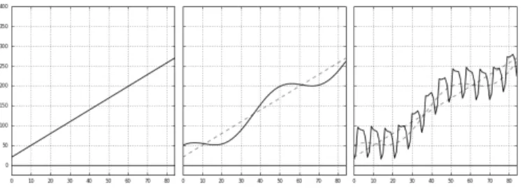
Fig. 1. Components of time series analysis.

of time. For example, we might count the number of visitors to a web site every hour. If we wish to determine when, if any, anomalies occurred over the last 10 days, we would create a TSA request with a granularity of hourly and a metric data array with the number of visitors for each hour over the previous 10 days. The total number of data points to analyze would be24×10or 240 data points.

Time series analysis is the statistical study of time series data [9], [10]. The analysis typically proceeds by decomposing the complex time series data into 4 simpler parts—trend, cyclicity, seasonality and irregular data referred to as error for ETS modeling. Time series analysis separates each of these components and examines them individually for their unique behaviors and characteristics. Once each component is modeled to the given degree of accuracy the individual models are recombined to produce an overall model.

Figure 1 illustrates how a given time series can be de-composed into the above mentioned components. Trend is the longest and most stable component of a time series representing increasing or decreasing aspects of a metric over time (Figure 1 (left)). ETS uses a linear approach to model this trend component. As such, we can think of trend as being identical to the simple linear equation y = mx+b, where m is the slope. Seasonality and cyclicity both represent mostly consistent oscillations over time (Figure 1 (middle)). The difference between cyclicity and seasonality is the time frame over which the oscillations are measured. Seasonality is typically viewed as oscillations with periods less than a year while cyclicity represents longer term oscillations, usually 2 to 5 years at a minimum. Since TSA limits analysis to at most a few years we use seasonality but not cyclicity in modeling time series.

Once trend and seasonality have been removed the remain-ing data consist of some unknown combination of error and valid measurements (Figure 1 (right)). Error can be attributed to a number of causes such as inaccurate measurement of the metric, missing data or unusual and unpredictable events.

TSA uses ETS to identify each of these three components and how they are combined—additive or multiplicative. A general additive model is shown in Equation 1

Y =T+C+S+E (1) whereas a general multiplicative model is

(5)

where T, C, S, and E denote trend, cyclicity, seasonality, and error, respectively. The decision to use the additive or the multiplicative model to decompose and/or recombine data is largely a matter of choice based on the specific application of both to a given time series and selecting the best fit.

IV. DIFFICULTIES INTESTING THETSA SOFTWARE

Automated testing of the TSA software is a crucial require-ment to ensure accuracy of results over the very large space of possible input time series. However, automation is very difficult to achieve due to the lack of a test oracle.

In order to conduct a test, the tester needs to first generate time series data (including the training and metric data) and then supply the remaining necessary parameters—such as granularity, confidence level, special days, etc, to form a valid TSA request, which will be passed to the TSA software. The TSA software will train itself using the training data and then return an output structure containing upper and lower bounds and the fitted data to model the input metric data.

To verify that the returned model is an acceptable fit for the input metric data a graphical representation of the inputs and the outputs is generated. The tester then looks at this graphic and subjectively decides if the results are acceptable or not. This is not always an easy determination to make as we have observed that different examiners will feel that different models reflect a better fit than others.

After the results are determined to be acceptable the tester will save the test case and the output to a testing repository for future regression testing. This entire process is not only time consuming and subjective but also severely limits the number and variety of time series inputs that can be covered.

V. A METAMORPHICTESTING(MT) SOLUTION

In order to automate testing we must be able to determine, for any given input, if the resulting model is an acceptable one without manual inspection. MT allows us to do this. The key to good metamorphic testing is finding useful metamorphic relations (MRs). For TSA testing we observe that a time series can be viewed as a two-dimensional rigid geometric object. By making this observation we are able to take advantage of an appropriate subset of geometric transformations as MRs.

A. Applying 2D Geometric Transformations as MRs

Geometric objects consist of points and lines. Rigid geo-metric objects have the property of maintaining the internal relationships of those points and lines as the object is shifted in the geometric space. For testing TSA we assume that every time series can be treated as a rigid two-dimensional (2D) geometric object. Further we define the 2D space by assigning the x-axis as timet and the y-axis as the metric value for a given time t.

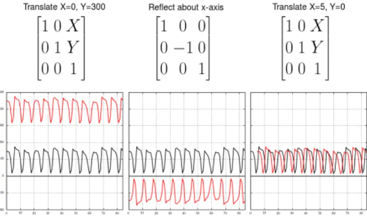
Geometric transformations describe the ways that geometri-cal objects can be moved within a geometric space. Geometric transformations can include the following: vertical translation, horizontal translation, reflection, rotation, scale and shear. Of these, vertical translation, horizontal translation and reflection

Fig. 2. Examples of geometric transformations.

preserve the internal relationships of points and lines without distortions.

If the assumption is made that all statistical models are derived from the internal relationships of the values of the time series and not from their relative or absolute position when represented in the plane we can safely expect that TSA will produce identical models regardless of orientation in space. As such the above mentioned geometric transformations make suitable choices for MRs.

A convenient and common way of applying geometric trans-formations to a given object is by using affine transformation matrices. Affine transformations preserve points, lines and planes. See Figure 2 for how the transformations of interest to TSA testing can be represented by 3x3 matrices, whereX and Y represent the increments in thex- andy-axes, respectively. Equation (3) illustrates how to apply the affine transformation to a time series by using matrix multiplication, wherey is the value of the time series at a given timex, andx0 andy0 are the new translated values.

  x0 y0 1  =   1 0 X 0 1 Y 0 0 1  ×   x y 1   (3) B. Testing Approach

To meet our goal of being able to fully automate TSA testing we needed to find a way to generate and verify arbitrarily complex time series data. Since all time series data can be decomposed into simple component parts—trend, cyclicity, seasonality, and error—our testing strategy began by generating simple time series data for two component parts, trend and seasonality. Trend data can be generated using a linear function y = mx where m is the slope of the line. Seasonal data can be generated using a periodic function y = Asin(Bx) where A (A > 0) is the amplitude and B affects the period. Although we could use more complex functions to construct the input time series data, in this study we only adopted the above simple approaches. We will show that even with such simple input data, MT is highly effective in revealing the defects in the TSA software.

If we represent a time series and its expected model as functionsf(x)andm(f(x)), respectively, then we can apply a

(6)

given geometric transformation to these two functions without changing the internal relationships of the data. Hence, the following conjecture (MR) is posited to hold:

Given a time series, f(x), and its expected TSA model,

m(f(x)), applying a geometric transformation T to f(x), denoted by T(f(x)), should have an expected TSA model

m(T(f(x))) that is equal toT(m(f(x))), that is:

T(m(f(x))) =m(T(f(x))). (4) While the above MR was identified from the users’ perspec-tive to reflect what a user would normally expect (and hence can be used for software validation [7]), the validity of the MR has also been confirmed by Adobe’s Data Science team and, hence, can be used for software verificationas well.1 A metamorphic test involves the executions of asource test case

and afollow-up test case[7]. To generate the source test cases, we create a base time series f(x) using the trend equation f(x) = mx or seasonality equation f(x) = Asin(Bx); to generate the follow-up test cases, we apply an affine transformation T to the base time series, namely, T(f(x)). This pair of f(x) andT(f(x)) are then converted into their respective TSA requests by further applying combinations of granularity, confidence level, training periods, etc. These requests are passed to the TSA service and the returned models are compared against the expected MR, namely, Equation 4.

Theoretically, both models (on the two sides of the above identity) returned by the TSA software could be erroneous in the same waydue to some software bugs—as a result, there is a chance that the above MR could still be satisfied when both models are incorrect. To detect this case, an additional check is done by comparing critical points in the model output against the input metric data, as will be explained in Section V-C.

C. Data Comparison Approaches

Due to the approximate nature of statistical modeling, exact equality is not always a reasonable expectation when conducting data comparison. In the simplest cases, where the time series is linear with no anomalies, mathematical equality to some given decimal point accuracy is a reasonable expectation. We limit the decimal place accuracy to 3 places after the decimal point. For general testing, a relative percent tolerance approach is best. With this method the two values have to agree to some test case supplied percentage. This method uses the formula |(a−b)/a| < v where v is the desired tolerance. A third approach we used is to compare the critical points for each model output—the fitted data, the upper bound, and the lower bound—with its input metric data. Critical points include the extrema (local and global maxima and minima) and inflection points. These critical points are found by calculating the first and second derivatives using Newton’s central difference formula. The derivative locations where there is a value of zero or where there is a change of sign from positive to negative or vice versa are compared. 1_Different _T _{of Equation 4 can result in different MRs. For ease of}

presentation, we will simply call Equation 4 “the expected MR” instead of “the expected group of MRs.”

The term drift has been coined to describe the variance in critical point locations. Drift is calculated using the Hamming distance.

VI. GENERATION OFMT TESTCASES

As explained previously, to generate the source test cases, we created base time series using the trend equation f(x) =

mxand the seasonality equationf(x) =Asin(Bx). After that affine transformations were applied to generate the follow-up time series.

A. Generation of Trend Test Cases

In this study, MT began by creating simple trended time series using y =mxfor x= 0,1, . . . ,99, as the base time series. The slope mis allowed to vary over the set of values

{1,000,100,10,1,0.5,0.1,0.01,0,−0.01,−0.1,−0.5,−1,

−10,−100,−1,000}.

To produce a geometrically transformed time series, the following vertical affine transformation matrix was applied to the base time series:

  1 0 X 0 1 Y 0 0 1  .

This matrix was used with X = 0 and Y taken from the set {1,000,000,000, 1,000, 100, 10,1, 0, −1, −10, −100,

−1,000,−1,000,000,000}.

For each pair of a base time series and one of its geometri-cally transformed time series, TSA requests were created using all combinations of the following TSA parameters:

• Granularity: Hourly, Daily, Weekly, Monthly. • Confidence:80%,85%,90%,95%,99%.

• Training period as a percentage of the time series data:

1%, 10%, 25%, 50%. For example, setting the training period to 10% means that the first 10% data points of the time series will be used as training data, and the remaining90%data points of the time series will be taken as the metric data to be modeled.

As a result, a large number of MT test case pairs (pairs of source and follow-up test cases) were generated for each pair of base and its geometrically transformed time series. In this study, we report on the use of the simplest test data where no anomalies were added to the time series, and the TSA parameters specifying weekend data, year over year data, or special days were not used. It was expected that such simple trend-only time series should result in nearly perfect equality, i.e., the model data in the two sides of Equation 4 should equal to 3 decimal place accuracy.

B. Generation of Seasonal Test Cases

For seasonal testing the equation y = Asin(Bx) for x= 0,1, . . . ,999was used to generate the base time series. A seasonal time series contains 1,000 instead of 100 data points. This is to provide more training data because a seasonal time series is more complex than a simple trended time series introduced in Section VI-A.

(7)

0 20 40 60 80 100 −10.6 −10.4 −10.2 −10.0 −9.8 −9.6 −9.4 metric_data 0 10 20 30 40 50 TC_H_80_0.5_0_-0.01_-10

Fig. 3. Example 1: Violation of MR detected by trend test cases. The right sub-figure shows that the two models (in red and blue) of Equation 4 diverged significantly.

We setAto be values taken from the set{10%×s,20%×s,

50%×s}, wheres is the size of the input time series. This was to make sure that the input time series would have an obvious seasonality and should not be confused with linear time series. The value ofBvaried over the range{1,0.5,0.1,

−0.1,−0.5,−1}.

To produce a geometrically transformed time series, the same type of vertical affine transformation matrix (as used for the trend test cases in Section VI-A) was applied to the base time series with X = 0 and Y taken from the set {1,000,000,000, 1,000, 100, 10, 1, 0, −1, −10, −100,

−1,000, −1,000,000,000}. The other TSA parameter set-tings were the same as for the trend test cases.

VII. TESTRESULTS

After execution of the test cases the log files were scraped to collect the complete TSA requests for any test case that failed to produce equality. This set of failed test case data was then fed to a script that produced graphical representations of the data for visual inspection.

A. Results of Trend Test Cases

Approximately 78% of the trend MT test cases reported an MR violation, hence revealing a failure. In this subsection we present some typical examples of the detected violations (failures).

The first example of MR violation is shown in Figure 3. The lines of Figure 3 (left) correspond to T(f(x))of Equation 4, where the red line corresponds to the training data and the green line corresponds to the metric data (i.e. data to model). The solid green lines of Figure 3 (left) and Figure 3 (right) are essentially the same; their slopes and positions are plotted differently because different scaling was applied to thex-axes, and also because the lines in Figure 3 (right) have been left shifted—since there is no need to show the training data in

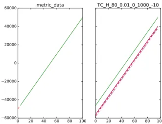
0 20 40 60 80 100 −60000 −40000 −20000 0 20000 40000 60000 metric_data 0 20 40 60 80 100 TC_H_80_0.01_0_1000_-10

Fig. 4. Example 2: Violation of MR detected by trend test cases. The right sub-figure shows that the two models of Equation 4 only differed slightly (as the blue lines are largely covered by their respective red lines) but they shifted away from the input metric data (the green line) quite significantly.

Figure 3 (right)—only the metric data are modeled in the output of the TSA software.

Consider Figure 3 (right), where the red and blue lines correspond to the source output (for the MT source test case) and follow-up output (for the MT follow-up test case), respectively. The solid, dashed, and dotted lines correspond to the upper bound, fitted data, and lower bound, respectively, returned by the TSA software to model the input metric data. According to the MR, the respective red and blue lines should be equal (overlap). But Figure 3 (right) shows that this was not the case. In other words, the MR was violated, as the red lines and blue lines diverged significantly. As a result, a failure was detected.

Figure 4 shows that a minor violation of MR can indicate a significant failure. Automatic numerical comparison to 3 decimal places revealed very small differences between the two models. Despite the small difference the failure was actually quite significant as both models significantly diverged from the input metric data.

Figure 5 (right) shows another example of MR violation where small differences were detected between the two mod-els. It is interesting to observe that the models (in particular the curvatures of the upper bounds) returned by the TSA software were somewhat periodic. This observation revealed a possible root cause of the failure: The TSA software might have applied an inappropriate model, which attempted to calculate seasonality, to the input metric data that were just a straight line.

The last example of MR violation detected with trend test cases is shown in Figure 6, where small differences between the two models were detected. This example differs from that of Figure 5 in that the former returned linear models without periodicity. This observation indicates that the TSA software might have (incorrectly) selected different models for the same

(8)

0 20 40 60 80 100 −60000 −40000 −20000 0 20000 40000 60000 metric_data 0 10 20 30 40 50 60 70 80 TC_D_99_0.25_0_1000_-1000

Fig. 5. Example 3: Violation of MR detected by trend test cases. In the right sub-figure, the two models (in red and blue) of Equation 4 differed slightly and the curvatures (especially the upper bounds) displayed certain periodicity although the input metric data were only a straight line (the green line).

0 20 40 60 80 100 −60000 −40000 −20000 0 20000 40000 60000 metric_data 0 20 40 60 80 100 TC_H_99_0.01_0_1000_-10

Fig. 6. Example 4: Violation of MR detected by trend test cases. In the right sub-figure, the two models (in red and blue) of Equation 4 differed slightly.

type of linear input metric data.

These examples of MR violations were sent to the Data Science team for review. Upon review it was noted that all these failed cases were returning models that were detecting seasonality, ANA or AAA. Since no seasonality was being added to the metric data this was an obvious problem. The reason for this faulty model selection was found to be due to the way the TSA software selected the best-fit model. The best fit was being determined by the comparison of the MAPE of each calculated model to a threshold value. This comparison was done sequentially after each model was returned. This resulted in the algorithmic error where the first model to have a MAPE less than the threshold value was taken as the best fit. That prevented the evaluation of any further models that might well result in an even lower MAPE. Because of this, the

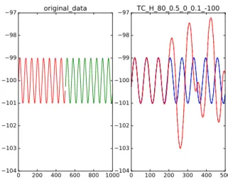
0 200 400 600 800 1000 −104 −103 −102 −101 −100 −99 −98 −97 original_data 0 100 200 300 400 500 −104 −103 −102 −101 −100 −99 −98 −97 TC_H_80_0.5_0_0.1_-100

Fig. 7. Example 5: Violation of MR detected by seasonal test cases. In the right sub-figure, the two models (in red and blue) of Equation 4 diverged significantly. 0 200 400 600 800 1000 −250 −200 −150 −100 −50 0 50 metric_data 0 100 200 300 400 500 TC_H_99_0.5_0_0.1_100_-100

Fig. 8. Example 6: Violation of MR detected by seasonal test cases. In the right sub-figure, the two models (in red and blue) of Equation 4 diverged significantly.

model that best fits trended data, AAN, was never evaluated. The detected bug was fixed by allowing all models to be executed first and then the model with the lowest MAPE was taken as the best fit. For all our trend test cases this resulted in correctly choosing the AAN model which had a MAPE of zero, that is, perfect fit where the upper and lower bounds and fitted data overlapped with the green line and the MR was fully satisfied.

B. Results of Seasonal Test Cases

Approximately 23% of the seasonal test cases returned an MR violation, of which some examples are shown in Figures 7, 8, and 9.

Figure 7 (left) shows the input training data (red) and metric data (green). Figure 7 (right) shows that an MR violation was

(9)

0 200 400 600 800 1000 −5 −4 −3 −2 −1 0 1 2 metric_data 0 100 200 300 400 500 TC_H_80_0.5_0_0.1_-1

Fig. 9. Example 7: Violation of MR detected by seasonal test cases. In the right sub-figure, the two models (in red and blue) of Equation 4 were completely different, revealing a new type of bug.

detected because the two models (in red and blue) diverged very significantly. Another example of MR violation is shown in Figure 8 (right), where differences between the two models (in red and blue) were obvious—this was caused by the bug reported in Section VII-A.

Figure 9 (right) shows a different type of behavior in MR violation, where the follow-up output (the blue lines) was completely different from the source output (where the solid, dashed, and dotted red lines overlapped). The blue lines clearly indicate a case where the TSA software was unable to find what would be considered a good model and defaulted to

functional filtering.

Again samples of the MR violations were passed to the Data Science team, who then confirmed that the violations were caused by multiple bugs in the TSA software. For example, the original design of the TSA algorithm would calculate models until one was found to be below some MAPE threshold value. But for the follow-up MT test case of Figure 9 (right), no model fell below the threshold; as such the TSA algorithm decided that if there was no good fit it would return functional filtering, hence producing the blue lines. The original algorithm has now been redesigned such that, if no model is below the MAPE threshold, functional filtering and its resulting MAPE will be added to the list of models. Then the model that has the lowest MAPE will be returned.

When examining the reported MR violations, another bug was also revealed. This bug caused erroneous modeling in the later parts of the red and blue lines of Figure 7 (right) and in the later parts of the red lines of Figure 9 (right).

After removal of all 3 bugs reported in this paper, the resulting TSA software produced accurate models when tested again, and the MR has been fully satisfied.

VIII. CONCLUSION ANDFUTUREWORK

In this paper we have reported our successful experience of applying MT to Adobe’s anomaly detection (TSA) software. The source test cases were very simple, including trend data generated using the linear functiony=mxand seasonal data generated using the periodic functiony=Asin(Bx). Despite the simplicity of these source test cases, the MR (namely, geometric transformation) has been proven highly effective as shown by the high violation rates. This study also suggests that geometric transformations can be used to identify useful MRs for the testing of other data analysis software of similar nature.

An investigation into the MR violations has revealed 3 bugs in the TSA software under test. These bugs include issues in bothverification(namely, erroneous implementation of the original algorithm) andvalidation(namely, defect in the original algorithm). The results of this study provide further evidence to support the observation that MT is an effective testing approach for both verification and validation [7].

In future work we plan to apply MT to Adobe software projects at a larger scale and further investigate the cost effectiveness of this testing paradigm and its combination with other testing methods.

ACKNOWLEDGMENTS

We would like to thank Dr. Jeff Berry of Adobe’s Data Science Department for his thoughtful input regarding the theoretical validity of the MR used in this study as well as his help with the preparation of the graphics of this paper.

REFERENCES

[1] E. T. Barr, M. Harman, P. McMinn, M. Shahbaz, and S. Yoo, “The oracle problem in software testing: A survey,”IEEE Transactions on Software Engineering, vol. 41, no. 5, pp. 507–525, 2015.

[2] C. E. Otero and A. Peter, “Research directions for engineering big data analytics software,”IEEE Intelligent Systems, vol. 30, no. 1, pp. 13–19, 2015.

[3] Z. Q. Zhou, S. Zhang, M. Hagenbuchner, T. H. Tse, F.-C. Kuo, and T. Y. Chen, “Automated functional testing of online search services,”Software Testing, Verification and Reliability, vol. 22, no. 4, pp. 221–243, 2012. [4] T. Y. Chen, S. C. Cheung, and S. M. Yiu, “Metamorphic testing: A new approach for generating next test cases,” Department of Computer Science, Hong Kong University of Science and Technology, Hong Kong, Tech. Rep. HKUST-CS98-01, 1998.

[5] T. Y. Chen, T. H. Tse, and Z. Q. Zhou, “Fault-based testing without the need of oracles,”Information and Software Technology, vol. 45, no. 1, pp. 1–9, 2003.

[6] S. Segura, G. Fraser, A. B. Sanchez, and A. Ruiz-Cort´es, “A survey on metamorphic testing,”IEEE Transactions on Software Engineering, vol. 42, no. 9, pp. 805–824, 2016.

[7] Z. Q. Zhou, S. Xiang, and T. Y. Chen, “Metamorphic testing for software quality assessment: A study of search engines,”IEEE Transactions on Software Engineering, vol. 42, no. 3, pp. 264–284, 2016.

[8] T. Y. Chen, F.-C. Kuo, W. Ma, W. Susilo, D. Towey, J. Voas, and Z. Q. Zhou, “Metamorphic testing for cybersecurity,”Computer, vol. 49, no. 6, pp. 48–55, 2016.

[9] R. Hyndman, A. B. Koehler, J. K. Ord, and R. D. Snyder,Forecasting with Exponential Smoothing. Springer-Verlag, 2008.

[10] D. C. Montgomery, C. L. Jennings, and M. Kulahci,Introduction to Time Series Analysis and Forecasting (Wiley Series in Probability and Statistics), 2nd ed. Wiley, 2015.