Doctoral Dissertations Student Theses and Dissertations
Fall 2011
Hilbert Transform applications in signal analysis and
Hilbert Transform applications in signal analysis and
non-parametric identification of linear and nonlinear systems
parametric identification of linear and nonlinear systems
Zuocai Wang
Follow this and additional works at: https://scholarsmine.mst.edu/doctoral_dissertations
Part of the Civil Engineering Commons
Department: Civil, Architectural and Environmental Engineering Department: Civil, Architectural and Environmental Engineering
Recommended Citation Recommended Citation
Wang, Zuocai, "Hilbert Transform applications in signal analysis and non-parametric identification of linear and nonlinear systems" (2011). Doctoral Dissertations. 2012.
https://scholarsmine.mst.edu/doctoral_dissertations/2012
This thesis is brought to you by Scholars' Mine, a service of the Missouri S&T Library and Learning Resources. This work is protected by U. S. Copyright Law. Unauthorized use including reproduction for redistribution requires the permission of the copyright holder. For more information, please contact [email protected].
HILBERT TRANSFORM APPLICATIONS IN SIGNAL ANALYSIS AND NON-PARAMETRIC IDENTIFICATION OF LINEAR AND NONLINEAR SYSTEMS
by
ZUOCAI WANG
A DISSERTATION
Presented to the Faculty of the Graduate School of the MISSOURI UNIVERSITY OF SCIENCE AND TECHNOLOGY
In Partial Fulfillment of the Requirements for the Degree
DOCTOR OF PHILOSOPHY in
CIVIL ENGINEERING
2011 Approved Genda Chen, Advisor
William Schonberg Roger A. LaBoube
Ian Prowell Xiaoping Du
2011 Zuocai Wang All Rights Reserved
ABSTRACT
Hilbert Huang Transform faces several challenges in dealing with closely-spaced frequency components, short-time and weak disturbances, and interrelationships between two time-varying modes of nonlinear vibration due to its mixed mode problem associated with empirical mode decomposition (EMD). To address these challenges, analytical mode decomposition (AMD) based on Hilbert Transform is proposed and developed for an adaptive data analysis of both stationary and non-stationary responses. With a suite of predetermined bisecting frequencies, AMD can analytically extract the individual components of a structural response between any two bisecting frequencies and function like an adaptive bandpass filter that can deal with frequency-modulated responses with significant frequency overlapping. It is simple in concept, rigorous in mathematics, and reliable in signal processing.
In this dissertation, AMD is studied for various effects of bisecting frequency selection, response sampling rate, and noise. Its robustness, accuracy, efficiency, and adaptability in signal analysis and system identification of structures are compared with other time-frequency analysis techniques such as EMD and wavelet analysis. Numerical examples and experimental validations are extensively conducted for structures under impulsive, harmonic, and earthquake loads, respectively. They consistently demonstrate AMD’s superiority to other time-frequency analysis techniques. In addition, to identify time-varying structural properties with a narrow band excitation, a recursive Hilbert Huang Transform method is also developed. Its effectiveness and accuracy are illustrated by both numerical examples and shake table tests of a power station structure.
ACKNOWLEDGMENTS
The author would like to express his sincere gratitude to Dr. Genda Chen for his continuing support, constant encouragement and invaluable advice throughout this research work. He would also like to thank Drs. William Schonberg, Roger A. LaBoube, Ian Prowell, and Xiaoping Du for their serving as Ph.D. committee members and for their continuing interest and encouragement.
Financial support to complete this study was provided in part by China Scholarship Council under Award No. NSCIS-2007-3020, by the U.S. National Science Foundation under Award No. CMMI0409420, and by Ameren Corporation. The results and opinions expressed in this dissertation are those of the author only and don’t necessarily represent those of the sponsors.
The author appreciates the opportunity provided by the Department of Civil, Architectural, and Environmental Engineering, Missouri S&T, to conduct and complete his research. He would also like to acknowledge the general support and help of Dr. Chen’s graduate students and visitor scholars in the course of research activities.
The author wishes to express his special and sincere gratitude to his wife, Qing Zhu, for her love, patience, understanding and assistance whenever needed. Last, but not the least, the author thanks his parents, parents-in-laws, sisters, brothers, and the previous academic advisor for their endless encouragement to pursue his degree.
TABLE OF CONTENTS Page ABSTRACT ... iii ACKNOWLEDGMENTS ... iv LIST OF ILLUSTRATIONS ... ix LIST OF TABLES ... xv SECTION 1. INTRODUCTION ...1
1.1. STRUCTURAL HEALTH MONITORING AND DAMAGE DETECTION ..1
1.2. STRUCTURAL PARAMETER IDENTIFICATION ...2
1.2.1. Frequency Domain. ...2
1.2.2. Time Domain...3
1.2.3. Time-Frequency Analysis. ...4
1.3. OBJECTIVES OF THIS STUDY ...6
1.4. RESEARCH SIGNIFICANCE ...7
1.5. DISSERTATION ORGANIZATION ...8
2. LITERATURE REVIEW ... 10
2.1. STRUCTURAL DYNAMICAL PARAMETERS ... 10
2.1.1. Natural Frequency. ... 10
2.1.2. Mode Shape, Mode Shape Curvature, and Modal Strain Energy. ... 11
2.1.3. Damping. ... 12
2.1.4. Nonlinear Feature. ... 12
2.2. PARAMETER IDENTIFICATION WITH CLOSELY-SPACED MODES .. 12
2.3. TIME-VARYING PARAMETER IDENTIFICATION ... 17
2.3.1. Least-Squares Based Method. ... 18
2.3.2. Wavelet Transform Based Method. ... 19
2.3.3. Hilbert Transform Based Method. ... 21
3. ANALYTICAL MODE DECOMPOSITION ... 24
3.1. HILBERT TRANSFORM AND ANALYTIC SIGNAL ... 24
3.2. HILBERT SPECTRAL ANALYSIS ... 25
3.2.2. Hilbert Spectra of Simple Functions... 26
3.3. EMD AND HHT ... 28
3.3.1. EMD. ... 28
3.3.2. HHT. ... 30
3.3.3. HHT Issues. ... 32
3.4. HILBERT VIBRATION DECOMPOSITION ... 34
3.4.1. Instantaneous Frequency of the Largest Energy Component. ... 34
3.4.2. Envelope of the Largest Energy Component. ... 35
3.5. BEDROSIAN THEOREM ... 37
3.5.1. Bedrosian Theorem Derivation. ... 37
3.5.2. Illustrative Examples. ... 38
3.6. A NEW SIGNAL DECOMPOSITION THEOREM ... 40
3.6.1. AMD Theorem and Proof. ... 40
3.6.2. Lowpass and Bandpass Filter Based on AMD Theorem. ... 42
3.6.3. Comparison with a Frequency Filtering Technique. ... 43
3.7. AMD FOR NONSTATIONARY SIGNALS... 46
3.7.1. AMD Theorem for Non-stationary Signals. ... 47
3.7.2. Role of Transform from Time Domain to Phase Domain. ... 49
3.7.3. Adaptive Lowpass and Bandpass Filter for Signals with Time- Varying Frequencies. ... 53
3.8. SUMMARY ... 55
4. PARAMETER IDENTIFICATION OF TIME INVARIANT SYSTEMS WITH AMD-HILBERT SPECTRAL ANALYSIS... 56
4.1. BISECTING FREQUENCY SELECTION ... 56
4.2. SIGNAL DECOMPOSITION IN ENGINEERING APPLICATIONS ... 58
4.2.1. Noise Effects. ... 59
4.2.2. Closely-Spaced Frequency Components. ... 61
4.2.2.1 Long period ocean wave... 61
4.2.2.2 Short period mechanical wave. ... 63
4.2.3. Amplitude Decaying Signals. ... 65
4.2.4. Small Intermittent Fluctuations around a Large Standing Wave. ... 66
4.3. MODAL PARAMETER IDENTIFICATION FROM FREE VIBRATION ... 68
4.3.2. Numerical Simulation. ... 70
4.4. MODAL PARAMETER IDENTIFICATION FROM FORCE VIBRATION 75 4.4.1. Transient Response ... 75
4.4.2. Numerical Examples with Harmonic Excitations. ... 77
4.4.2.1 Single-DOF system. ... 78
4.4.2.2 3-DOF mechanical system. ... 82
4.5. MODAL PARAMETER IDENTIFICATION FROM AMBIENT VIBRATION ... 85
4.5.1. The RDT-AMD Method. ... 86
4.5.2. Parametric Study of RDT-AMD Method. ... 87
4.5.2.1 Frequency space index. ... 87
4.5.2.2 Effect of free vibration time duration... 91
4.5.3. Application of the RDT-AMD Method. ... 94
4.5.3.1 3-DOF mechanical system with closely-spaced modes. ... 94
4.5.3.2 36-story shear building with light appendage... 96
4.6. SHAKE TABLE TEST VALIDATION ... 101
4.7. SUMMARY ... 105
5. IDENTIFICATION OF TIME-VARYING AND WEAKLY NONLINEAR SYSTEMS WITH AMD-HILBERT SPECTRAL ANALYSIS ... 108
5.1. HHT, WAVELET AND AMD-HILBERT SPECTRAL ANALYSIS ... 108
5.1.1. AMD-Hilbert Spectral Analysis. ... 108
5.1.2. Comparative Study on Instantaneous Frequency. ... 108
5.2. PARAMETRIC STUDIES ... 112
5.2.1. Bisecting Frequency Selection. ... 112
5.2.2. End Effect Reduction. ... 114
5.2.3. Sampling Rate Selection and Noise Effect. ... 114
5.3. SIGNAL DECOMPOSITION WITH FREQUENCY AND AMPLITUDE MODULATED COMPONETS ... 118
5.3.1. Frequency Modulated Components. ... 118
5.3.2. Frequency and Amplitude Modulated Components. ... 120
5.4. INSTANTANEOUS FREQUENCY IDENTIFICATION OF WEAKLY NONLINEAR SYSTEMS ... 123
5.4.2. Frequency Traction for Two-Story Shear Building. ... 125
5.4.3. Frequency Traction for a Duffing System. ... 127
5.4.4. Frequency Traction for a Hysteretic Nonlinear System. ... 129
5.4.4.1 Free vibration. ... 129
5.4.4.2 Ambient vibration. ... 133
5.5. SUMMARY ... 136
6. TIME-VARYING SYSTEM IDENTIFICATION UNDER KNOWN EXCITATIONS WITH HHT METHOD... 138
6.1. HHT METHOD FOR TIME-VARYING SYSTEM IDENTIFICATION .... 138
6.1.1. Identification of Parameter Variation. ... 138
6.1.2. A Recursive HHT Method for Multi-Story Shear Buildings. ... 139
6.1.3. Evaluation of Identification Accuracy. ... 142
6.2. APPLICATION OF THE RECURSIVE HHT METHOD ... 143
6.2.1. Single-Story Shear Building. ... 143
6.2.2. Two-Story Shear Building. ... 144
6.2.2.1 Case 1: Abruptly reduction stiffness. ... 145
6.2.2.2 Case 2: Gradually reducing stiffness... 147
6.2.2.3 Case 3: Periodically reducing stiffness. ... 147
6.3. SUMMARY ... 148
7. TIME-VARYING SYSTEM IDENTIFICATION OF HIGH VOLTAGE SWITCHES OF A POWER SUBSTATION ... 149
7.1. INTRODUCTION OF THE SHAKE TABLE TEST ... 149
7.2. TEST SETUP AND INSTRUMENTATION ... 150
7.3. SYSTEM IDENTIFICATION WITH WEAK VIBRATION... 153
7.4. TIME-VARYING PARAMETER IDENTIFICATION WITH THE RECURSIVE HHT METHOD ... 154
7.5. ULTIMATE BEHAVIOR TEST OF THE STRUCTRUE ... 157
7.6. SUMMARY ... 160
8. CONCLUSIONS ... 161
BIBLIOGRAPHY... 164
LIST OF ILLUSTRATIONS
Figure Page
1.1. Relationship between Excitation and Response……….. 2
2.1. A Signal with Closely-Spaced Frequency and Its Fourier Spectrum ... 13
2.2. Decomposed Signals by Bandpass Filtering versus Exact Signals ... 14
2.3. A Dynamic Signal with Sudden Drop Frequency ... 17
3.1. Instantaneous Amplitude, Phase Angle and Frequency in Complex Plane ... 25
3.2. Original Signal and Its Hilbert Transform ... 26
3.3. Fourier and Hilbert Spectra ... 26
3.4. Original Signal and Its Hilbert Transform ... 27
3.5. Fourier and Hilbert Spectra ... 27
3.6. Original Signal with Two Cosine Frequency Modulated Components ... 29
3.7. First Four IMFs of the Original Signal ... 30
3.8. Block Diagram of the HHT Process ... 31
3.9. Hilbert Spectrum of Two Cosine Frequency Modulated Components ... 32
3.10. The First Two IMFs by EMD ... 33
3.11. Two Instantaneous Frequencies by HHT ... 34
3.12. Block Diagram of Hilbert Vibration Decomposition... 36
3.13. Integration Region ... 38
3.14. Hilbert Transform of Product Signals ... 39
3.15. Block Diagram of a Lowpass Filter with a Bisecting Frequency ... 42
3.16. Block Diagram of a Bandpass Filter with Two Bisecting Frequencies ... 43
3.17. Decomposed Signals by AMD ... 44
3.18. Fourier Spectra of the Decomposed Signals by AMD ... 44
3.19. Decomposed Signals by Frequency Filtering and Exact Signals ... 46
3.20. Illustration on Varying Bisecting Frequencies in Time Domain ... 47
3.21. Illustration on Varying Bisecting Frequencies in Phase Domain ... 49
3.22. Component Frequencies and Bisecting Frequency ... 50
3.23. The Decomposed Lowpass and Exact Signal in Time Domain ... 51
3.25. Variation of ∫ - with Bisecting Frequency Selection. ... 52
3.26. Fourier Spectra of Individual Components in Time Domain ... 53
3.27. Fourier Spectra of Individual Components in Phase Domain ... 53
3.28. Block Diagram of an Adptive Lowpass Filter with a Time Varying Bisecting Frequency ... 54
3.29. Block Diagram of an Adaptive Bandpass Filter with Two Time Varying Bisecting Frequencies... 54
4.1. Fourier Spectra of Time Series in Six Cases ... 57
4.2. Effect of Bisecting Frequency Selection on Amplitude Ratio ... 58
4.3. IMF3 and IMF4 by EMD versus Exact Signals ... 59
4.4. Fourier Spectra of IMF3 and IMF4 by EMD ... 60
4.5. Decomposed Signals by AMD versus Exact Signals ... 60
4.6. Fourier Spectra of the Decomposed Signals by AMD versus Exact Signals ... 60
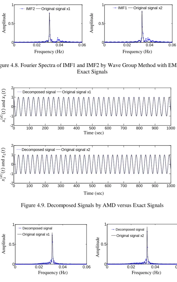
4.7. IMF1 and IMF2 by the Wave Group Method with EMD versus Exact Signals ... 61
4.8. Fourier Spectra of IMF1 and IMF2 by Wave Group Method with EMD and Exact Signals ... 62
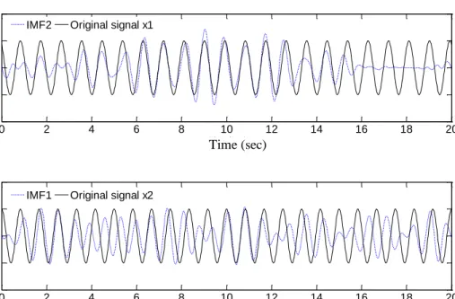
4.9. Decomposed Signals by AMD versus Exact Signals ... 62
4.10. Fourier Spectra of the Decomposed Signals by AMD versus Exact Signals ... 62
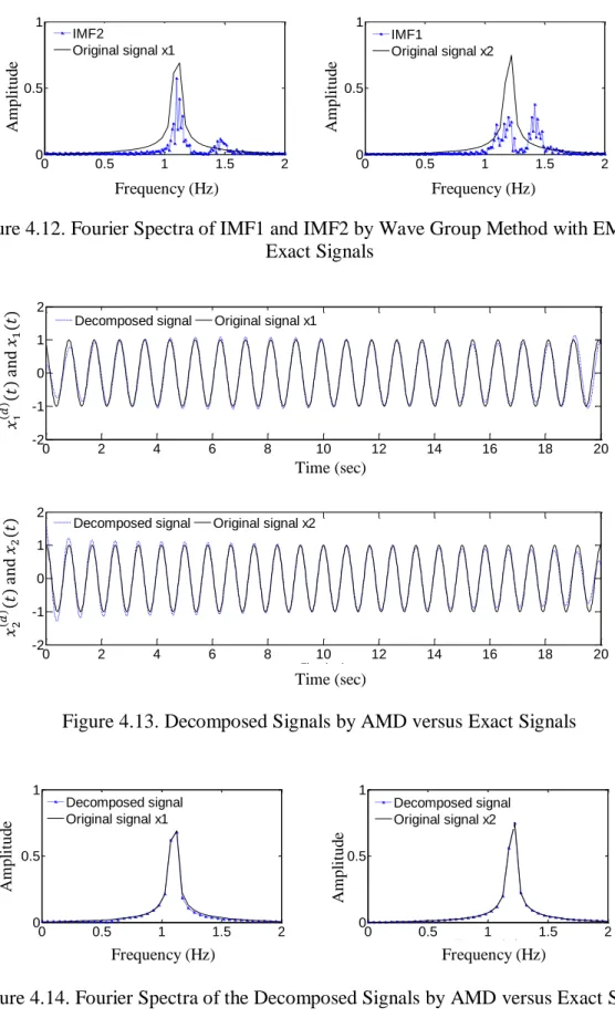
4.11. IMF1 and IMF2 by the Wave Group Method with EMD versus Exact Signals ... 63
4.12. Fourier Spectra of IMF1 and IMF2 by Wave Group Method with EMD and Exact Signals ... 64
4.13. Decomposed Signals by AMD versus Exact Signals ... 64
4.14. Fourier Spectra of the Decomposed Signals by AMD versus Exact Signals ... 64
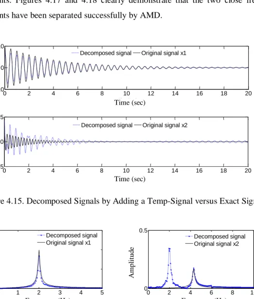
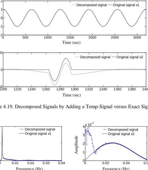
4.15. Decomposed Signals by Adding a Temp-Signal versus Exact Signals ... 65
4.16. Fourier Spectra of the Decomposed Signals by Adding a Temp-Signal versus Exact Signals ... 65
4.17. Decomposed Signals by AMD versus Exact Signals ... 66
4.18. Fourier Spectra of the Decomposed Signals by AMD versus Exact Signals ... 66
4.19. Decomposed Signals by Adding a Temp-Signal versus Exact Signals ... 67
4.20. Fourier Spectra of the Decomposed Signals by Adding a Temp-Signal versus Exact Signals ... 67
4.21. Decomposed Signals by AMD versus Exact Signals ... 68
4.23. Representative Fourier Spectrum of a Structural Response ... 69
4.24. 3-DOF Representation of a Mechanical System ... 71
4.25. Three Modes of Vibration Decomposed by AMD ... 71
4.26. Fourier Spectra of the Decomposed Modes of Vibration by AMD ... 72
4.27. Amplitude and Phase angle of Hilbert Transforms ... 73
4.28. Instantaneous Mode Shapes Identified From the Amplitude of Hilbert Transforms74 4.29. Fourier Transform of Three Modes of Vibration Decomposed by AMD ... 75
4.30. Displacement, Velocity, and Acceleration Responses ... 78
4.31. Fourier Spectra of Displacement, Velocity, and Acceleration Responses ... 79
4.32. Extracted Transient and Steady State Displacement by AMD ... 80
4.33. Fourier Spectra of Transient and Steady State Displacement ... 80
4.34. Amplitude and Phase Angle of Analytic Signal ... 80
4.35. Displacement Response with 10% Gaussian White Noise ... 81
4.36. Extracted Noise Polluted Transient and Steady State Displacement by AMD ... 81
4.37. Fourier Spectra of Noise Polluted Transient and Steady State Displacement ... 82
4.38. Amplitude and Phase Angle of Analytic Signal with 10% Noise ... 82
4.39. Displacement at m3 ... 83
4.40. Fourier Spectrum of Displacement at m3 ... 83
4.41. Extracted Transient and Steady State Displacement using AMD ... 84
4.42. Extracted Modal Responses from the Transient Displacement using AMD ... 84
4.43. Amplitude and Phase Angle of the Modal Responses ... 85
4.44. Two-Story Building Example... 88
4.45. Exact and Decomposed Responses of the First Mode from AMD and Bandpass Filtering Methods ... 89
4.46. Energy Error Indices Associated with AMD and Bandpass Filtering Methods ... 91
4.47. Fourier Spectra of the Exact Responses of Modes 1 and 2 and Their Overlapping . 91 4.48. Fourier Spectra of Ambient Vibration and Free Vibration after RDT... 93
4.49. Energy Error Indices under Free Vibration ... 93
4.50. Decomposed and Exact Mode 1 Response with Time Duration: 1, 5, 10, 15, and 20 sec. ... 93
4.51. Ambient Displacement and Extracted Free Response ... 94
4.53. Decompose Modes from Extracted Free Response using AMD ... 95
4.54. Amplitude and Phase Angle of Hilbert Transform of the Free Response Obtained by RDT ... 96
4.55. Shear Building with Light Appendage... 97
4.56. Simulated Excitation and Response ... 97
4.57. Fourier Spectrum of the Acceleration at the Top of Appendage ... 98
4.58. Closely-Spaced Modal Responses ... 99
4.59. Fourier Spectra of Closely-Spaced Modal Response ... 99
4.60. Extracted Free Response using RDT ... 99
4.61. Amplitude and Phase Angle of the Free Vibration Response Extracted from Ambient Vibration ... 100
4.62. The Shake Table Test Setup ... 102
4.63. Base Motions to the Structure with Various Excitations ... 103
4.64. Measured Top Floor Accelerations of the Structure ... 103
4.65. Fourier Spectra of the Measured Top Floor Accelerations ... 104
4.66. Extracted Free Vibration Responses ... 104
4.67. Amplitude and Phase Angle of the Free Vibration Response Extracted from the Third Floor Acceleration ... 105
5.1. First Two IMFs from EMD ... 109
5.2. Instantaneous Frequency from HHT... 109
5.3. Wavelet Transform Scalograms for Various Center Frequencies ... 111
5.4. Decomposed Signals using AMD ... 111
5.5. Instantaneous Frequency from AMD-Hilbert Spectral Analysis and Wavelet Analysis ... 113
5.6. AMD-Hilbert Spectrum Analysis with Various Bisecting Frequency Selections.... 113
5.7. Contaminated Signal with Noise and the Gaussian White Noise ... 116
5.8. Continuous Wavelet Analysis: Scalogram and Bisecting Frequencies ... 116
5.9. Instantaneous Frequencies with Various Sampling Rates ... 116
5.10. Fourier Spectra of the Gaussian Noise with Different Sampling Rates... 117
5.11. Fourier Spectra of the Decomposed Signals with Different Sampling Frequencies... 117
5.12. Instantaneous Frequencies with Different Noises ... 118
5.14. Continuous Wavelet Transform Scalogram and Bisecting Frequencies ... 119
5.15. Decomposed Signals by AMD ... 120
5.16. Instantaneous Frequencies Obtained from AMD and Wavelet Ridges ... 120
5.17. Original Signal ... 121
5.18. Continuous Wavelet Transform Scalogram and Bisecting Frequencies ... 122
5.19. Decomposed Signals by AMD ... 122
5.20. Instantaneous Frequencies Obtained from AMD and Wavelet Ridges ... 122
5.21. Two-Story Shear Building ... 125
5.22. Decomposed Modal Responses by AMD ... 126
5.23. Instantaneous Frequencies by AMD ... 127
5.24. Free Response and Its Fourier Spectrum of a Duffing System ... 128
5.25. Identified Dynamic Characteristics of the Analytic Signal ... 128
5.26. A One-Story Shear Building with a Tuned Mass Damper ... 129
5.27. Free Vibration Responses of Linear and Nonlinear Systems ... 131
5.28. Fourier Spectra of Free Responses of Linear and Nonlinear Systems ... 131
5.29. Instantaneous Frequencies of Mode 1 and 2 Responses from ... 131
5.30. Bouc-Wen Hysteretic Loops with Various Initial Displacements... 132
5.31. Phases of the Decomposed First Modal Response via AMD ... 132
5.32. Damage Index E from Free Vibration... 133
5.33. Ambient Responses of Nonlinear and Linear Systems ... 134
5.34. Fourier Spectra of Ambient Responses of Nonlinear and Linear Systems ... 134
5.35. Instantaneous Frequencies of the Analytical Signal of Mode 1 and 2 Decomposed from via AMD ... 134
5.36. Bouc-Wen Hysteretic Loops with Various Excitations ... 135
5.37. Phases of the Decomposed First Modal Responses via AMD ... 135
5.38. Damage Index E from Ambient Vibration ... 136
6.1. Multi-Story Shear Building ... 140
6.2. Displacement Time History of the Stiffness-Varying Building ... 144
6.3. Identified Stiffness of the Single-Story Building ... 144
6.4. Two-Story Shear Building ... 145
6.6. Identified Stiffness Based on One IMF ... 146
6.7. Identified Stiffness from the Recursive Method: Case 1 ... 146
6.8. Identified Damping Coefficient from the Recursive Method: Case 1 ... 146
6.9. Identified Stiffness from the Recursive Method: Case 2 ... 147
6.10. Identified Stiffness from the Recursive Method: Case 3 ... 147
7.1. Typical Damage Resulting from Earthquakes... 150
7.2. Test Setup of the High Voltage Switch on Shake Table (all units: mm) ... 151
7.3. Wood Truss System ... 151
7.4. Two Data Acquisition Systems ... 152
7.5. Fundamental Frequency and Damping Ratio Identified from the First Test ... 153
7.6. Fundamental Frequency and Damping Ratio Identified from the Second Test ... 154
7.7. Average Relative Displacement from First and Second Tests ... 154
7.8. Measured Responses and Identified Parameters from the 1st Test ... 156
7.9. Measured Responses and Identified Parameters from the 2nd Test ... 157
7.10. Displacements Measured from LVDT 7 and LVDT 8: First Test at 7.2 Hz ... 158
7.11. Displacements Measured from LVDT 7 and LVDT 8: First Test at 7.0 Hz ... 158
7.12. Displacements Measured from LVDT 7 and LVDT 8: Third Test ... 159
7.13. Overall View of the Failed Structure ... 159
LIST OF TABLES
Table Page
4.1. Identified Natural Frequencies and Damping Ratios by AMD ... 73
4.2. Identified Natural Frequencies and Damping Ratios from Force Vibration ... 85
4.3. Properties of the Two-Story Building ... 88
4.4. Identified Natural Frequencies and Damping Ratios from Ambient Vibration ... 96
4.5. Identified Natural Frequency and Damping Ratio of Building-Appendage System 100 4.6. Modal and Physical Properties of Steel Frame and Damper ... 102
4.7. Identified Natural Frequencies and Damping Ratios from the Top Floor Acceleration ... 105
1.INTRODUCTION
1.1.STRUCTURAL HEALTH MONITORING AND DAMAGE DETECTION
Structural health monitoring has been an active research field since more than ten years ago. Its overall goal is to provide a diagnosis and prognosis tool for structural condition at any moment during the service life of an engineering structure. It includes several main steps such as sensor deployment, data acquisition, feature extraction, and condition evaluation. Techniques in structural health monitoring can be classified into local and global groups, depending upon the space coverage of damage detection. The local group is used to detect any local damage on a small part of the structure. Often referred to as nondestructive evaluation, this group of techniques includes acoustics emission, hardness testing, and thermal field mapping. These methods all require that the vicinity of the damage is known a priori and that the portion of a structure being inspected must be accessible. Due to these limitations, the local techniques are often limited to the damage detection on or near the surface of the structure. The global group of technologies can be applied to assess the system condition of complex structures. They are dominated by the examination of changes in vibration characteristics.
Vibration-based methods for system identification and damage detection have been widely studied as summarized in a comprehensive review by Doebling et al. (1996; 1998). The basic idea is that the modal parameters such as natural frequencies, mode shapes, and modal damping are functions of the physical properties of the structure such as mass, damping, and stiffness. Therefore, changes in physical property will cause changes in the modal properties. The main advantage of vibration-based methods is that measurements at one location are sufficient to assess the condition of the whole structure.
More recently, Sohn et al. (2004) described the vibration-based structural health monitoring in four parts: (1) operational evaluation, (2) data acquisition, fusion, and cleansing, (3) feature extraction and data compression, and (4) statistical model development for feature discrimination. Operational evaluation begins to understand the purposes of structural monitoring, unique aspects of a structure, and unique features of the damage that is to be detected. The data acquisition process involves selecting the types of sensors, sensor locations, the number of sensors, data acquisition, storage, etc.
Then, data fusion means to integrate information from disparate sources and assess threats on the basis of data coming in from different sources (Klein, 1999). Data cleaning is a process of accepting and rejecting data in the feature selection process. For example, filtering has been widely used to filter out the noise component of measurements. Feature extraction is a process of identifying damage sensitive properties from vibration measurements. These properties can be used to distinguish damage from the undamaged structure.
1.2.STRUCTURAL PARAMETER IDENTIFICATION
A critical step for vibration-based structural health monitoring is to extract dynamic features such as natural frequencies, mode shapes, and damping ratios from structural responses. This step is often referred to as structural parameter identification. Structural parameter identification involves various methods in frequency domain such as frequency response method, in time domain such as least-squares estimation method and stochastic subspace method, and in time-frequency domain such as wavelet transform and Hilbert transform based methods. The identified structural parameters can serve as an index in structural damage detection, condition assessment, vibration mitigation, and long-term health monitoring.
1.2.1. Frequency Domain. With the development of digital signal processing
techniques such as Fast Fourier Transform (FFT), modal tests and analysis become competitive in modal property characterization of structures (Alvin et al., 2003). In order to determine modal parameters, the frequency response function of a structure between its excitation and structural response is estimated from the available vibration measurements. It can be readily derived from their Fourier transforms as illustrated in Figure 1.1.
Figure 1.1. Relationship between Excitation and Response Measured Excitation Excitation Noise Actual Excitation Actual Response Response Noise Measured Response FRF(ω) F (ω) Z(ω) M(ω) Y(ω) X(ω) N(ω)
In Figure 1.1, F(ω) and X(ω) represent the Fourier transforms of the measured excitation and the measured response, respectively; Z(ω) = F(ω) - M(ω) is the Fourier transform of the actual excitation and Y(ω) = X(ω) - N(ω) is the Fourier transform of the actual response; M(ω) and N(ω) represent the mechanical and measurement noises to the
input and structural response, respectively; FRF(ω) is the frequency response function of
the structural system. Mathematically, the response Y(ω) can be related to the excitation Z(ω) by:
(1.1)
According to Trendafilova (1998) and Monaco et al. (2000), frequency response functions can be used to quantify and localize minor damage. However, they face difficulties when the input excitation is unknown with ambient vibration of structures. In this case, Brincker et al. (2000; 2001) developed a frequency domain decomposition method under two assumptions: (1) white noise input, and (2) lightly structural damping. Singular value decomposition (SVD) can then be applied to expand the power spectrum density matrix of output responses into the same form as conventional matrix decomposition in modal analysis. Consequently, a first-order linear approximation of the output power spectrum density matrix is used for the estimation of mode shapes and damping coefficient. Although powerful for closed-spaced natural frequency identification, SVD requires the availability of pre-selected natural frequencies and is applicable only when the assumptions are valid.
1.2.2. Time Domain. Structural parameter identification in time domain includes
a number of computationally efficient techniques such as least-squares estimation, Auto-Regressive Moving-Average (ARMA), and natural excitation technique (NExT). Least-squares estimation has been widely applied to system identification (Benedettini et al., 1995; Loh et al., 1995; Smyth et al., 1999; Lin et al., 2001; Yang and Lin, 2005). For example, Smyth et al. (1999) presented an adaptive estimation approach for the on-line identification of hysteretic systems under arbitrary dynamic loading. Yang (2005) introduced a new adaptive tracking technique to identify time-varying structural parameters. These methods placed more weight on the current data point and thus introduced a forgetting factor on the previous data so that their effect is reduced.
Natural frequencies, mode shapes, and damping ratios can be identified from a multivariate ARMA model derived from the equation of motion of a structural system. This model has been extensively studied in the last two decades (Lee and Yun, 1991; He and Roeck, 1997). Without knowing the exact degrees of freedom of the system, it often produces more eigenvalues than the actual number of frequencies (Bodeux and Golinval,
2000).Therefore, only some of the estimated eigenvalues are associated with the modes
of vibration. To distinguish the physical from nonphysical modes, Bodeux and Golinval (2000) presented a prediction error identification scheme to evaluate the model parameters for vibration-based damage detection.
The NExT method was developed by James et al. (1995; 1996) to effectively extract modal parameters from ambient vibration. Under the white noise excitation, a cross-correlation function between the stationary responses at two degrees of freedom of a system resembles the free vibration of the system and can thus be used to identify the system parameters. For mode shapes, one of the degree of freedom must be used as a reference point. In combination with the Eigen-system Realization Algorithm, Caicedo et al. (2004) further applied this method to the IASC-ASCE benchmark problem. However, two significant issues cannot be overlooked for a proper implementation of this technique: (1) a stationary pink noise excitation, and (2) an independent reference signal of the measured responses. In many applications with ambient vibration, a long record of data is required. However, if the record is too long, the assumption for stationary responses may no longer be justifiable.
1.2.3. Time-Frequency Analysis. Most of the structural parameter identification works in time domain or in frequency domain have been focused on time invariant linear systems. In recent years, researchers embarked on the parameter identification of time-varying linear systems or nonlinear systems that are of great interest in the damage detection of engineering structures. In this case, measured responses are typically non-stationary and modal parameters in frequency domain change over time. As such, time-frequency analysis of measured responses has been developed to decompose and analyze non-stationary signals.
During the last two decades, wavelet analysis and Hilbert transform have been attracting wide attention in the structural health monitoring community. The interest to
the topic of time-frequency analysis is still rising as evidenced by the increasing number of papers published in technical journals and conference proceedings.
Wavelet analysis can be viewed as Fourier spectral analysis with adjustable time windows (Chui, 1992; Flandrin, 1999) for a non-stationary data series. Due to the introduction of adjustable windows, wavelet analysis provides multiple levels of details and approximations in time-frequency domain so that transient features of the data series can be retained in the frequency characteristics. As a result, it has been widely applied to non-stationary dynamic signal analysis (Staszewski, 1997; Ruzzene et al., 1997; Gurly and Karrem, 1999; Hou et al., 2000; Kijewski and Kareem, 2002; 2003). Even so, wavelet analysis still has several issues. For example, wavelet analysis is a non-adaptive data analysis tool since the basic wavelet remains unchanged with the signal characteristics. It also has the so-called leakage problem due to limited length of the basic wavelet function. Therefore, in the time-frequency plane, the frequency curves are often smeared in a large range especially at low frequency. To extract distinct time-frequency curves, Wang and Ren (2007) presented a SVD based wavelet ridge extraction method for further signal analysis and reconstruction. However, according to the Heisenberg-Gabor uncertainty principle, a signal cannot be concentrated on an arbitrary small time-frequency region. In other words, it is impossible to achieve high resolution both in time and frequency domain.
More recently, empirical mode decomposition (EMD) was developed by Huang et al. (1998; 1999; 2003) to decompose a stationary and non-stationary data series into a finite number of intrinsic mode functions (IMFs), each having a well-behaved Hilbert transform. The well-known Hilbert-Huang transform (HHT) combines EMD with Hilbert spectral analysis; it is an adaptive data analysis tool for non-stationary signals. Some HHT applications in engineering, biomedical, financial and geophysical data analyses have been presented by Huang and Shen (2005) and Huang and Attoh-Oine (2005). More research about the EMD applications in signal processing can be found in Chen and Feng (2003), Yang et al. (2004), Peng et al. (2005), Shi and Law (2007), Shi et al. (2009), and
Zheng et al. (2009). Although powerful in extracting the properties of non-stationary
signals, EMD still faces several challenges in some engineering applications: 1) difficult to decompose signals with closely-spaced frequency components such as wave groups in
ocean engineering, free vibration and beating responses in structural and mechanical systems, 2) difficult to separate a short time weak signal from a stationary strong response, and 3) impossible to deal with the time-varying feature between two modes of vibration for nonlinear systems. Attempts have been made by a few investigators to address these challenges (Chen and Feng, 2003; Peng et al., 2005; and Zheng et al., 2009). However, it is still quite a challenge to consistently and reliably extract individual components from a non-stationary response when their time-varying frequencies are closely spaced, particularly resulting from a nonlinear structural system.
1.3.OBJECTIVES OF THIS STUDY
To address the above challenges, analytical mode decomposition (AMD) is sought to accurately decompose any signal to physically meaningful components in various engineering applications. Therefore, the main objective of this study is to develop a signal decomposition theorem based on the Hilbert transform of a harmonics multiplicative time series, which will serve as the foundation for AMD in structural health monitoring. It decomposes a time series into many signals whose Fourier spectra are non-vanishing over mutually-exclusive frequency ranges separated by constant bisecting frequencies for stationary and non-stationary signals with no overlapping component frequencies, and by time-varying bisecting frequencies for non-stationary signals with overlapping component frequencies.
The performance of AMD with constant bisecting frequencies in dealing with the closely-spaced modes of vibration of linear structures will be investigated with stationary, transient, and intermittent signals both numerically and experimentally. For structural parameter identification, AMD in combination with Hilbert spectral analysis is demonstrated with the free vibration and harmonic vibration of a three degree-of-freedom (DOF) mechanical system and the ambient vibration of a 36-story building with a 4-story light appendage. AMD will then be applied to identify the modal properties of a ¼-scale 3-story building frame with closely-spaced modes due to the presence of multiple tuned mass dampers based on a series of shake table tests.
The performance of AMD with time-varying bisecting frequencies will be investigated with non-stationary, frequency-modulated signals. In this case, each
frequency modulated individual component between any two bisecting frequencies can be analytically extracted. The signal decomposition theorem developed in this study will be demonstrated to function like an adaptive bandpass filter that allows a complete pass of frequency band between two adjacent bisecting frequencies. Parametric studies will be conducted for bisecting frequencies selection, sampling rate and noise effects. Representative engineering applications will be studied with frequency gradually varied, amplitude and frequency modulated, and nonlinear shear buildings under impulsive, harmonic, white noise and earthquake loads. Unlike EMD, AMD is simple in concept, rigorous in mathematics, efficient in computation, and reliable in signal processing. The time-varying bisecting frequencies will be applied to the parametric identification of nonlinear systems.
The secondary objective of this study is to develop a recursive time-varying parameter identification method under narrow band excitations based on Hilbert transform. To validate the proposed method, time-varying parameters will be identified for 1- and 2-story buildings with three scenarios of time-varying parameters: abrupt, gradual, and periodical stiffness variations under earthquake excitations. Noise effects will be taken into account in numerical simulations. The method will be applied to identify a real-world high voltage switch structure from shake table test data. The high voltage switch includes a friction mechanism for opening and closure of the switch.
1.4.RESEARCH SIGNIFICANCE
The critical issue for parameter identification is to extract useful information from the field measured data sets. This requires a robust and high performance signal analysis methodology. Although vibration-based methodologies have been extensively investigated for time-invariant structural systems during the last two decades, there are still several challenges as mentioned above, particularly for systems with closely-spaced modes of vibration. Therefore, a reliable signal processing method is quite necessary to address these challenges.
Recently, parameter identification for time-varying structures has received considerable attention. Some methods such as least-squares based techniques are accurate but inefficient. Other methods such as HHT are inaccurate for MDOF systems.
Therefore, it is highly important to develop a methodology that can accurately and efficiently identify the parameters of time-varying structural systems.
When subjected to extreme loads such as tornados and earthquakes, a structure may experience damage. One of the important objectives in structural health monitoring of civil infrastructures is to identify the state of the structure and to detect damage as it occurs. The damage of the structure is reflected by a local change of structural parameters. Hence, it is important to develop methodologies that are capable of detecting structural parameter changes.
1.5.DISSERTATION ORGANIZATION
This dissertation consists of eight sections. In Section 1, the concepts of structural health monitoring and structural parameter identification are introduced. The objectives and significance of this study are presented. In Section 2, the state-of-the-art development in system identification is reviewed particularly for time-varying parameters of linear and nonlinear systems. In Section 3, a signal decomposition theorem with Hilbert transform or AMD in structural health monitoring is discovered and demonstrated to have addressed the challenges associated with EMD or those of Hilbert vibration decomposition (HVD).
The theorem is applied to identify the time-invariant parameters of various structures with closely-spaced modes from free, harmonic and ambient vibration in Section 4. In particular, AMD is combined with the conventional random decrement technique (RDT) to develop a new system identification method with ambient vibration, referred to as the RDT-AMD method. The new method is applied to a 3-DOF mechanical system and a 36-story building with 4-story appendage system, both with closely-spaced modal frequencies, demonstrating its effectiveness in practical applications. Finally, its accuracy in modal parameter identification is validated with shake table testing of a 3-story building. Parametric studies are conducted to investigate the bisecting frequency selection and frequency resolution of the new method.
In Section 5, AMD is extended to the time-varying parameter identification of from non-stationary responses of both linear and nonlinear systems. Its aim is to lay a mathematical foundation for the decomposition of amplitude- and frequency-modulated
signals and establish admittance requirements for the selection of time-varying bisecting frequencies, one between any two adjacent modulated frequencies. Parametric studies are conducted to understand and quantify the effects of bisecting frequency selection, signal frequency overlapping, sampling rate, and signal noise. Time-varying modal parameters of a nonlinear shear building under impulsive, white noise and earthquake loads will be tracked using the mathematically rigorous theorem.
In Section 6, in order to track the variation of structural parameters under force vibration, a recursive HHT method is developed. It allows the structural identification of a building story-by–story and thus is computationally efficient in the determination of both stiffness and damping coefficients. The method is validated with one- and two-story buildings with three types of time-varying parameters (abruptly, gradually, and periodically) under earthquake excitations even when a simulated measurement noise up to 5% of the signal intensity was injected to the building responses.
In Section 7, the parameter identification and ultimate behavior of a time-varying power station structure are extensively studied based on shake table test results. A series of harmonic tests with constant amplitude and increasing excitation frequency is conducted. Modal parameters are identified for each excitation frequency based on the proposed recursive HHT approach.
In Section 8, the main findings and conclusions of this study are summarized and further researches on AMD and time-varying system identification are recommended.
2.LITERATURE REVIEW
The focus of this study is to develop an adaptive data analysis method for the parameter identification of structures with closely-spaced modes, time-varying properties, and hysteretic behaviors. Therefore, structural dynamic parameters and their role in structural health monitoring are briefly reviewed.
2.1.STRUCTURAL DYNAMICAL PARAMETERS
The actual implementation of a vibration-based structural health monitoring starts with designing a dynamic experiment. The type and number of sensors, and sensor placement are first decided so that physical quantities of interest can be measured. Then, some damage sensitive properties or structural parameters are extracted from the measured dynamic responses. The critical issue in feature extraction is to identify the appropriate dynamic parameters for a particular application, such as natural frequencies, mode shapes, damping, and nonlinear properties. All these parameters play a significant role in system identification and damage detection.
2.1.1. Natural Frequency. Natural frequency is one of the basic dynamic
properties of structures. The amount of literature related to system identification and damage detection with frequency shifts is quite large (Loland and Dodds, 1976; Vandiver, 1977; Cawley and Adams, 1979; Ismail, et al., 1990; Stubbs and Osegueda, 1990a; 1990b; Skjaerbaek, et al., 1996; Leutenegger et al., 1999).
The observation that changes in structural properties cause changes in vibration natural frequencies was the impetus for the intensive research works in structural health monitoring. For example, Loand and Dodds (1976) used the changes in the resonant frequencies, mode shapes, and response spectra to identify damage of an offshore oil platform. Frequency changes of 10% to 15% were observed when a structural modification was implemented to resemble a structural failure near the waterline. They concluded that change in response spectrum can be used to monitor structural integrity. However, Farrar, et al. (1994) conducted a dynamic test on the I-40 bridge and found that when the cross-section stiffness at the center of a main plate girder had been reduced 96.4%, no significant reduction in the modal frequencies was observed. In general,
natural frequency represents global behavior of a structural system. Depending on the redundancy, the influence of local damage on the change in natural frequency may change. As such, the appropriateness of using frequency shift as a damage indicator must be evaluated case by case.
2.1.2. Mode Shape, Mode Shape Curvature, and Modal Strain Energy. West
(1984) first used the mode shape to locate structural damage without a prior finite element model. The author first used the modal assurance criteria to ensure the level of mode correlation between the conventional test and acoustic test of an undamaged space shuttle orbiter body flap. The mode shapes evaluated from the measured displacements or accelerations of a structure were then used to detect existing damage. Similar approaches have been taken by other researchers such as Stanbridge et al. (1997) and Ettouney (1998). Their research concluded that change in mode shape can be used to detect the location of damage with acceptable accuracy. However, whether this method is applicable for real-world structures is yet to be seen because the number of mode shapes and natural frequencies that can be reliably identified from experiments is quite limited.
Mode shape curvature is basically the second derivative of the mode shape with respect to the location coordinate. Pandey et al. (1991) demonstrated that absolute changes in mode shape curvature can be used for damage detection for beam like structures. It is more sensitive to damage than the mode shape itself. However, the derivative of mode shape is also sensitive to noise. In addition, numerical evaluation on the second derivative of mode shapes sometimes caused unacceptable errors. Therefore, Chance et al. (1994) used the measured strain instead to evaluate curvature directly, improving its accuracy significantly.
Mode strain energy is another potential damage indicator. The ith modal strain
energy in the jth element stiffness is defined by the ith mode shape and element stiffness
kj, which is . Its fraction of the total modal strain energy is defined as the ith modal
strain energy ratio for the jth element. The difference in element modal strain energy ratio
before and after damage can be used to detect the structural damage. The studies based on the modal strain energy for damage detection (Carrasco et al., 1997; Choi and Stubbs, 1997) demonstrated that the modal strain energy method performed very well for damage location in truss, beam, and plate structures. In all cases, the modal strain energy method
needs information from the undamaged structure. Therefore, a baseline model is required to apply this method.
2.1.3. Damping. Damping is another important dynamic property of structures.
Change in damping has been used to detect nonlinear effects caused by cracking (Modena et al., 1999; Adhikari and Woodhouse, 2001). However, damping has not been used as extensively as natural frequencies and mode shapes in structural health monitoring due mainly to its excessive variation. The large variation is likely attributed to the fact that damping effect is a complicated phenomenon in structural dynamics; its mechanism is unclear in many applications. Although viscous or complex damping has been widely considered in structural dynamics textbooks for convenience in mathematical derivation, real-world structures can have significant friction and inelastic deformation effects. Therefore, further research is needed in order to use damping as a damage indicator in structural health monitoring.
2.1.4. Nonlinear Feature. Stiffness and damping force nonlinearities can
introduce dynamic phenomena and behaviors that are dramatically different from those predicted by the linear theory. Brandon (1997; 1999) stated that the nonlinear response of a mechanical system was often overlooked and valuable information was lost when one discarded the time series data and focused on the spectral data. Therefore, the author advocated the use of time-domain system identification techniques such as ARMA model and autocorrelation function to retain the important nonlinear information. Although a few attempts were made to take advantage of nonlinear behaviors (Vakakis et al., 2004; Kershenc et al., 2005), it is still a challenge to identify a nonlinear system due to its highly individualistic nature.
2.2.PARAMETER IDENTIFICATION WITH CLOSELY-SPACED MODES
With the development of signal decomposition techniques, such as fast Fourier transform, wavelet transform, and Hilbert transform, various methods in frequency domain and for time-frequency analysis have become competitive in modal property characterization. Over the past decades, a vast amount of literature based on Fourier transform, wavelet transform, and Hilbert transform can be found for the time-invariant modal parameter identification of linear structures (Doebling et al., 1996; Sohn et al.,
2004). Most of them, however, faced a challenge in identifying the modal parameters of a structure with closely-spaced modes, particularly in the presence of measurement noise. Following is a detailed discussion of such a challenge and research needs to address it.
A classical approach in frequency domain is just to take the discrete Fourier transform of dynamic responses and estimate the well separated modes of vibration directly from the peaks of power spectral density functions (Bendat and Piersol, 1993). In the case of close modes, it is difficult to distinguish two nearby peaks. For example,
consider a 20 second time duration dynamic response signal of
, where , and .
The three frequencies were set to f11.1 Hz, f2 1.2 Hz, and f31.3 Hz with a
frequency spacing of 0.1 Hz. A sampling rate of 50 point per second is used. The original signal and its Fourier spectrum are presented in Figure 2.1.
Figure 2.1. A Signal with Closely-Spaced Frequency and Its Fourier Spectrum
The time series of finite length was first transformed into the frequency domain using the Fourier transform. The Fourier spectrum was then filtered with a bandpass filter to potentially separate the mode information. Finally, the filtered Fourier spectrum was transformed back to the time domain with the inverse Fourier transform. Both in time and
0 2 4 6 8 10 12 14 16 18 20 -4 -2 0 2 4 0 0.5 1 1.5 2 0 0.5 1 0 2 4 6 8 10 12 14 16 18 20 -4 -2 0 2 4 0 0.5 1 1.5 2 0 0.5 1 Time (sec) x ( t ) Frequency (Hz) A m pl it ud e
(a) Original Signal
frequency domains, a finite length signal is equivalent to the application of a rectangular window on its corresponding infinite long signal. Both transforms introduce numerical errors in two ways: signal modification by windowing and end effect due to sharp edges or brick walls of the windows. Applying a rectangular window in the frequency/time domain is equivalent to execute a convolution between a sinc function and the time/frequency function over an infinite range. This means that the time/frequency function is now a distorted signal, therefore, the brick wall with the rectangular window or the sudden change of frequency corresponds to an infinitely long oscillation in the time domain that cannot be represented accurately with the Fourier transform and its inverse transform. An improper selection of the beginning and end of a signal could introduce an artificial oscillation as illustrated in Figure 2.2. In the case of splitting closely-spaced frequency components, there is no space to soften the brick wall by designing two smooth edges of a window.
Figure 2.2. Decomposed Signals by Bandpass Filtering versus Exact Signals
0 2 4 6 8 10 12 14 16 18 20 -2 0 2 0 2 4 6 8 10 12 14 16 18 20 -2 0 2
Decomposed signal Original signal x1
Decomposed signal Original signal x2
0 2 4 6 8 10 12 14 16 18 20 -2 0 2 0 2 4 6 8 10 12 14 16 18 20 -2 0 2
Decomposed signal Original signal x1
Decomposed signal Original signal x2
0 2 4 6 8 10 12 14 16 18 20 -3 -2 -1 0 1 2 3 Time (Sec) D e co m p o se d a n d o ri g in a l si g n a l 0 2 4 6 8 10 12 14 16 18 20 -2 0
2 Decomposed signal Original signal x3
Time (sec) x1 ( t ) Time (sec) x2 ( t ) Time (sec) x3 ( t )
In order to detect closely-spaced modes, Brincker et al. (2001) presented a singular value decomposition method in frequency domain under two assumptions: (1) white noise input, and (2) lightly structural damping. In this case, the output power spectrum density matrix can be separated into the effects of a set of single DOF systems, each corresponding to an individual mode from which the mode shapes and damping can be estimated. By using the decomposition technique, closely-spaced modes were identified with high accuracy even in the case of strong noise contamination of the dynamic measurements.
Wavelet transform as one of the time-frequency analysis tools has attracted wide attention in recent years. This method has been widely applied to structural modal parameter identification (Lardies et al., 2002; Kijewski et al., 2003; Yan et al., 2006; Min et al., 2009). However, for a structure with closely-spaced modes, it is difficult to select appropriate wavelet parameters such as center frequency and bandwidth to distinguish the closely-spaced modes. Attempts have been made by a few investigators to identify close-spaced modes with wavelet transform. Teng and Zhu (2010) used an adaptive genetic algorithm to optimize the parameters of wavelet including the center frequency and its bandwidth. The parameters of wavelet were optimized with the adaptive genetic algorithm, whose objective function is the standard deviation between the wavelet ridge and fitting line. In doing so, their numerical simulations with three closely-spaced modes demonstrated that the wavelet transform in combination with the adaptive genetic algorithm can be used to identify the closely-spaced modes of vibration.
HHT is another time-frequency analysis method developed for stationary and non-stationary signal analysis and has been widely applied in structural parameter identification and damaged detection. However, central to HHT, the EMD sift process is unable to decompose signals with closely-spaced modes. With the HHT method, Chen and Xu (2002) explored the possibility to identify the modal parameters of a structure with closely-spaced modes. For the structure with closely-spaced modes, the cutoff frequencies determined from the power spectrum density of the measured response time history were used in the signal sifting process with the intermittency check. The random decrement technique was further applied to each of the modal responses decomposed by EMD with the cutoff frequency intermittency check to obtain the free modal responses.
Then, the modal parameters such as naturel frequencies and damping ratios can be identified. The results of their research show that damping ratios identified using the HHT method is much more accurate than those from the fast Fourier transform analysis.
Wang (2005) presented another HHT based method to decompose a signal with close frequency components. A temporary complex time series was introduced to shift down the frequencies of its components. This can greatly increase the ratio between the higher and lower frequencies so that individual components can be separated with EMD. The key point of this method is to increase the ratio of the frequencies of two components. Consider a signal with two cosine functions:
(2.1)
in which and is a phase angle. The ratio of the two frequencies is .
It can be increased by subtracting a temporary frequency in the numerator and
denominator simultaneously. The ratio between the two downshifted frequencies
becomes . To achieve this downshifting process, a complex
analytic signal is defined as:
(2.2)
in which, represents Hilbert transform of the function in the bracket and √ is
an imaginary unit. Downshifting in frequency components can be achieved by
multiplying an exponential function, , to yield a new complex signal:
(2.3)
For a proper , can be as large as 1.5, and the new
complex signal can be easily separated by EMD:
∑ (2.4)
in which is the kth decomposed component named as intrinsic mode function, and
is a residual function. The decomposition of the original analytical complex signal can
then be upshifted back by multiplying with both sides of Equation (2.4):
∑
(2.5)
Therefore, the decomposition of original signal can be expressed as:
∑
(2.6)
in which, represents the real part of the complex function in bracket. Although
between two frequencies decreases, particularly for flexible structures such as long-span bridges with very low natural frequencies. Overall, it is still a challenge to consistently and reliably identify the properties of structures with closely-spaced modes.
2.3.TIME-VARYING PARAMETER IDENTIFICATION
The measured dynamic responses in structural and mechanical systems are often irregular in amplitude and frequency over time, which is referred to as amplitude- and frequency-modulated signals. Such responses must be characterized with time-varying features such as instantaneous frequency. For example, consider a dynamic response with
a sudden drop of frequency: { , the original signal and its
Fourier spectrum are presented in Figure 2.3. It can be seen from Figure 2.3 that the Fourier spectrum loses the time essence of frequency drop at 5 sec, which is important in real time structural health monitoring. To enable the identification of damage location and occurrence, least-squares based methods in time domain have recently been applied into time-varying parameter identification. Advanced time-frequency analysis techniques such as wavelet transform and Hilbert transform have also been used as summarized below.
Figure 2.3. A Dynamic Signal with Sudden Drop Frequency
0 1 2 3 4 5 6 7 8 9 10 -2 0 2 0 1 2 3 4 5 6 7 8 9 10 -2 0 2 0 1 2 3 4 5 0 0.5 1 Time (sec) x ( t ) Frequency (Hz) A m pl it ud e
(a) Original Signal
2.3.1. Least-Squares Based Method. Least-squares estimation is a computationally efficient approach in time domain and has been widely applied to structural system identification (Bendedettine et al.; 1995, Bodson, 1995; Loh and Tou, 1995; Smith et al., 1997; Yongkyu, 2002; Ravindra, 2006). A constant forgetting factor is commonly used in the above methods. For example, Smyth et al. (1999; 2002) and Lin et al. (2001) presented a modified least-squares method for the on-line identification of
hysteretic systems under arbitrary dynamic loading. The drawback of the constant
forgetting factor approach is a trade-off between tracking ability and noise sensitivity. A smaller factor allows a more accurate tracking on the variation of structural parameters but makes the approach more sensitive to noise effect.
Yang and Lin (2005) presented a new adaptive tracking technique based on the least-squares estimation approach to identify time-varying structural parameters. Their method is able to track the abrupt changes of structural parameters due to damage. The tracking algorithm is based on the adaptation of the current measure data to determine the parameter variations and the covariance of the residual error is only contributed by measurement noises. Their proposed approach was applied to linear structures, such as the Phase I ASCE structural health monitoring benchmark building and a nonlinear elastic structure. Yang et al. (2006; 2007) further detected damage to structures using the adaptive tracking technique with unknown excitations. Simulation results for a Duffing-type nonlinear ASCE benchmark building demonstrated that the method is quite effective and accurate for tracking the variations of structural parameters due to damage.
Yang et al. (2009) further proposed a new least-squares based method, referred to as the adaptive quadratic sum-squares error, for the online system identification and damage detection of structures. This new technique can be briefly described as follows.
The error vector at time ( is a sampling time) between the observation data
and the theoretical data is a nonlinear function of the unknown parametric vector . The
error vector was linearized for at the previous time step , so that is a
linear function of unknown parametric vector . Consequently, the sum-squares error
becomes a quadratic function of . The analytical recursive solution for the estimate ̂ of
can then be obtained by minimizing the quadratic sum-squares error. The simulation results, including a two-story steel frame finite element model, a plane truss with finite
element model, and a 5-DOF hysteretic shear beam building, demonstrated the accuracy of the method in tracking the variation of structural parameters such as stiffness degradation due to damage. The adaptive quadratic sum-squares error method was further developed by Huang et al. (2010). The advantage of this method is that the unknown parametric vector is directly estimated and the state vector is updated, thus reducing computational efforts. The accuracy and effectiveness of the proposed method was demonstrated by numerical simulations and the experimental data taken from a scaled three-story building model.
More recently, Wang and Chen (2011) developed a moving-window curve fitting method based on the least-squares estimation in each fixed window. Central to the new method is the transformation from a dynamic to static problem by integrating the dynamic measurements and loads over time. This method can be applied to locate and quantify multiple cracks and sudden reductions in stiffness in beam-like structures. It is a computationally efficient, straightforward identification method for multi-span continuous highway bridges.
2.3.2. Wavelet Transform Based Method. Wavelet transform as an advanced
time-frequency analysis technique has been designed for non-stationary time signals of linear systems in the past two decades. Wavelet analysis is essentially an advanced short-time Fourier transform method with adjustable windows at various short-times. Due to its flexibility in window length selection, wavelet analysis reveals the detail and approximation of a time signal at multiple levels and retains the transient characteristics of the data series with time-frequency spectral decomposition. The integral wavelet
transform is the convolution of a signal and the conjugate of a scaled parent wavelet
function with a dilation scale a>0 and translational value b:
√ ∫ (
) (2.7)
in which is inversely proportional to frequency, is the wavelet coefficient that
represents the similitude between the dilated and shifted parent wavelet and the signal at
time b and scale , and * represents an operation of complex conjugate. The distribution
of the wavelet coefficient in time-frequency plane can be used for signal time-frequency analysis. In particular, the extracted ridge lines can be used for signal reconstruction.
Gurly and Kareem (1999) used wavelet transform to decompose a random process into localized orthogonal basis functions, providing a convenient format for the modeling, analysis, and simulation of non-stationary processes. The time-frequency analysis of wavelet transform provided insight into the characteristics of transient signals. The analysis of non-stationary signals including wind, wave and earthquake applications was typically accomplished by the continuous wavelet transform in Equation (2.7).
Staszewski (1997) compared the cross section procedure, impulse response recovery procedure, and ridge detection procedure in damping identification of a dynamic system. The wavelet transform was used to decouple the system into single harmonic modes. The mathematical framework of the decoupling procedure was presented.
Hou et al. (2000) presented a wavelet-based approach for structural health monitoring and damage detection. Both numerical simulation for a simple structural mode with breakage springs and actual recorded data of the building response during an earthquake event were analyzed. The results demonstrated that structural damage or a change in system stiffness can be detected by spikes in the details of the wavelet decomposition of the response data. The locations of the spikes can accurately indicate the time instances when the structural damage occurred.
Kijewski and Kareem (2003) argued that civil engineering structures usually possess long period motions and thus require finer frequency resolution of parent wavelets. Although many parent wavelets are available, the authors focused on the Morlet wavelet due to its unique properties in continuous wavelet transform. The Morlet wavelet is defined by:
(2.8)
It is essentially a Gaussian-windowed Fourier transform with harmonic oscillations at the
central frequency of . In their study, Kijewski and Kareem (2003) demonstrated that a
proper selection of Morlet wavelet central frequencies is required to balance modal separation. In doing so, the instantaneous frequency of a signal can be identified from the wavelet phase or from the ridges of the amplitude.
Although widely used in signal processing, wavelet analysis is non-adaptive to a particular data series. It depends upon the introduction of a predetermined parent wavelet. Therefore, some of the highly transient features in a time signal may be lost in the