package psychomix
Hannah Frick, Carolin Strobl, Friedrich Leisch,
Achim Zeileis
Working Papers in Economics and Statistics
2011-21
University of Innsbruck
http://eeecon.uibk.ac.at/
The series is jointly edited and published by
-Department of Economics
-Department of Public Finance
-Department of Statistics Contact Address:
University of Innsbruck Department of Public Finance Universitaetsstrasse 15 A-6020 Innsbruck Austria Tel: + 43 512 507 7171 Fax: + 43 512 507 2970 e-mail: [email protected]
The most recent version of all working papers can be downloaded at http://eeecon.uibk.ac.at/wopec/
psychomix
Hannah Frick Universit¨at Innsbruck Carolin Strobl Universit¨at Z¨urich Friedrich Leisch Universit¨at f¨ur Bodenkultur Wien Achim Zeileis Universit¨at Innsbruck AbstractMeasurement invariance is an important assumption in the Rasch model and mixture models constitute a flexible way of checking for a violation of this assumption by detecting unobserved heterogeneity in item response data. Here, a general class of Rasch mixture models is established and implemented in R, using conditional maximum likelihood esti-mation of the item parameters (given the raw scores) along with flexible specification of two model building blocks: (1) Mixture weights for the unobserved classes can be treated as model parameters or based on covariates in a concomitant variable model. (2) The distribution of raw score probabilities can be parametrized in two possible ways, either using a saturated model or a specification through mean and variance. The function raschmix() in the R package psychomix provides these models, leveraging the general infrastructure for fitting mixture models in the flexmix package. Usage of the function and its associated methods is illustrated on artificial data as well as empirical data from a study of verbally aggressive behavior.
Keywords: mixed Rasch model, Rost model, mixture model, flexmix,R.
1. Introduction
In item response theory (IRT), latent traits are usually measured by employing probabilis-tic models for responses to sets of items. One of the most prominent examples for such an approach is the Rasch model (Rasch 1960) which captures the difficulty (or equivalently eas-iness) of binary items and the respondent’s trait level on a single common scale. Generally, a central assumption of most IRT models (including the Rasch model) is measurement invari-ance, i.e., that all items measure the latent trait in the same way for all subjects. If violated, measurements obtained from such a model provide no fair comparisons of the subjects. A typical violation of measurement invariance in the Rasch model is differential item functioning (DIF), seeAckerman(1992).
Therefore, assessing the assumption of measurement invariance and checking for DIF is crucial when establishing a Rasch model for measurements of latent traits. Hence, various approaches have been suggested in the literature that try to assess heterogeneity in (groups of) subjects either based on observed covariates or unobserved latent classes. If covariates are available, classical tests like the Wald or likelihood ratio test can be employed to compare model fits between some reference group and one or more focal groups (Fischer and Molenaar 1995). Typically, these groups are defined by the researcher based on categorical covariates or
arbi-trary splits in either numerical covariates or the raw scores (Andersen 1972). More recently, extensions of these classical tests have also been embedded into a mixed model representation (Van den Noortgate and De Boeck 2005). Another recently suggested technique is to recur-sively define and assess groupings in a data-driven way based on all available covariates (both numerical and categorical) in so-called Rasch trees (Strobl, Kopf, and Zeileis 2011).
Heterogeneity occuring in latent classes only (i.e., not observed or captured by covariates), however, is typically addressed by mixtures of IRT models. Specifically,Rost(1990) combined a mixture model approach with the Rasch model. If any covariates are present, they can be used to predict the latent classes (as opposed to the item parameters themselves) in a second step (Cohen and Bolt 2005). More recently, extensions to this mixture model approach have been suggested that encompass this prediction, seeTay, Newman, and Vermunt (2011) for a unifying framework.
In this paper, we introduce thepsychomixpackage for theRsystem for statistical computing (RDevelopment Core Team 2011) that provides software for fitting a general and flexible class of Rasch mixture models along with comprehensive methods for model selection, assessment, and visualization. The package leverages the general and object-oriented infrastructre for fitting mixture models from theflexmix package (Leisch 2004; Gr¨un and Leisch 2008), com-bining it with the functionRaschModel.fit()from the psychotoolspackage (Zeileis, Strobl, and Wickelmaier 2011) for the estimation of Rasch models. All packages are freely available from the ComprehensiveRArchive Network athttp://CRAN.R-project.org/.
The reason for using RaschModel.fit() as opposed to other previously existing (and much more powerful and flexible)Rpackages for Rasch modeling – such asltm(Rizopoulos 2006) or eRm(Mair and Hatzinger 2007) – is reduced computational complexity: RaschModel.fit()is intended to provide a “no frills” implementation of simple Rasch models, useful when refitting a model multiple times in mixtures or recursive partitions (see alsoStroblet al. 2011). Whilepsychomixwas under development, anotherRimplementation of theRost(1990) model became available in packagemRm(Preinerstorfer 2011). As this builds on specialized C++
code, it runs considerably faster than the genericflexmix approach – however, it only covers this one particular type of model and offers fewer methods for specifying, inspecting, and as-sessing (fitted) models. Inpsychomix, both approaches are reconciled by optionally employing themRmsolution as an input to theflexmix routines.
In the following, we first briefly review both Rasch and mixture models and combine them in a general Rasch mixture framework (Section 2). Subsequently, the R implementation in psychomix is introduced (Section 3), illustrated by means of simulated data, and applied in practice to a study of verbally aggressive behavior (Section 4). Concluding remarks are provided in Section5.
2. Rasch mixture models
In the following, we first provide a short introduction to the Rasch model, subsequently outline the basics of mixture models in general, and finally introduce a general class of Rasch mixture models along with the corresponding estimation techniques.
2.1. The Rasch model
Sucess of solving an item or agreeing with it is coded as “1”, while “0” codes the opposite response. The model suggested byRasch(1960) uses the person’s abilityθi(i= 1, . . . , n) and
the item’s difficultyβj (j= 1, . . . , m) to model the response yij of personito itemj:
P(Yij =yij|θi, βj) =
exp{yij(θi−βj)}
1 + exp{θi−βj}
. (1)
Under the assumption of independence – both across persons and items within persons (see
Fischer and Molenaar 1995, Chapter 1) – the likelihood for the whole sample y = (yij)n×m
can be written as the product of the likelihood contributions from Equation 1 for all com-binations of subjects and items. It is parameterized by the vector of all person parameters
θ= (θ1, . . . , θn)> and the vector of all item parameters β = (β1, . . . , βm)> (see Equation 2).
On the basis of the number of correctly solved items, the so-called “raw” scoresri=Pmj=1yij,
it can be factorized into a conditional likelihood of the item parameters h(·) and the score probabilties g(·) (Equation 3). Because the scores r are sufficient statistics for the person parameters θ, the likelihood of the item parameters β conditional on the scores r does not depend on the person parametersθ (Equation4).
L(θ, β) = f(y|θ, β) (2) = h(y|r, θ, β)g(r|θ, β) (3) = h(y|r, β)g(r|θ, β). (4) The conditional likelihood of the item parameters takes the form
h(y|r, β) = n Y i=1 exp{−Pm j=1yijβj} γri(β) (5)
whereγri(·) is the elementary symmetric function of order ri, capturing all possible response
patterns leading to a certain score (seeFischer and Molenaar 1995, Chapter 3, for details). There are several approaches to estimating the Rasch model: Joint maximum likelihood (ML) estimation ofβ andθ is inconsistent, thus two other approaches have been established. Both are two-step approaches but differ in the way the person parameters θ are handled. For marginal ML estimation a distribution for θ is assumed and integrated out in L(θ, β), or equivalently ing(r|θ, β). In theconditional MLapproach only the conditional likelihood of the item parametersh(y|r, β) from Equation 5 is maximized for estimating the item parameters. Technically, this is equivalent to maximizing L(θ, β) with respect to β if one assumes that
g(r|δ) =g(r|θ, β) does not depend on θorβ, but potentially other parameters δ.
In R, the ltm package (Rizopoulos 2006) uses the marginal ML approach while the eRm package (Mair and Hatzinger 2007) employs the conditional ML approach, i.e., uses and reports only the conditional part of the likelihood in the estimation ofβ. The latter approach is also taken by the RaschModel.fit() function in the psychotools package (Zeileis et al.
2011).
2.2. Mixture models
Mixture models are a generic approach for modeling data that is assumed to stem from different groups (or clusters) but group membership is unknown.
The likelihoodf(·) of such a mixture model is a weighted sum (with prior weightsπk) of the
likelihood from several componentsfk(·) representing the different groups:
f(yi) = K X
k=1
πkfk(yi).
Generally, the components fk(·) can be densities or (regression) models. Typically, all
k components fk(·) are assumed to be of the same type f(y|ξk), distinguished through their
component-specific parameter vectorξk.
If variables are present which do not influence the components fk(·) themselves but rather
the prior class membership probabilities πk, they can be incorporated in the model as
so-called concomitant variables (Dayton and Macready 1988). In the psychometric literature, such covariates predicting latent information are also employed, e.g., by Tay et al. (2011) who advocate a unifying IRT framework that also optionally encompasses concomitant infor-mation (labeled MM-IRT-C for mixed-measurement IRT with covariates). To embed such concomitant variablesxi into the general mixture model notation, a model for the component
membership probabilityπ(k|xi, α) with parameters α is employed:
f(yi|xi, α, ξ1, . . . , ξK) = K X
k=1
π(k|xi, α)f(yi|ξk) (6)
where commonly a multinomial logit model is chosen to parametrizeπ(k|xi, α) (see e.g.,Gr¨un and Leisch 2008;Tayet al. 2011). Note that the multinomial model collapses to separateπk
(k= 1, . . . , K) if there is only an intercept and not real concomitants in xi.
2.3. Flavors of Rasch mixture models
When combining the general mixture model framework from Equation6with the Rasch model based on Equation 1, several options are conceivable for two of the building blocks. First, the component weights can be estimated via a separate parameterπk for each component or
via a concomitant variable model π(k|xi, α) with parameters α. Second, the full likelihood
function f(yi|ξk) of the components needs to be defined. If a conditional ML approach is
adopted, it is clear that the conditional likelihoodh(yi|ri, β) from Equation 5 should be one
part, but various choices for modeling the score probabilities are available. One option is to model each score probability with its own parameter g(ri) = ψri, while another (more
parsimonious) option would be to adopt a parametric distribution with fewer parameters (Rost and von Davier 1995). Note that while for a single-component model, the estimates of the item parameters ˆβ are invariant to the choice of the score probabilities (as long as it is independent fromβ), this is no longer the case for a mixture model withK≥2.
Rost’s original parametrization
One of these possible mixtures – the so-called “mixed Rasch model” introduced by Rost
(1990) – is already well-established in the psychometric literature. It models the score proba-bilities through separate parametersg(ri) =ψri (under the restriction that they sum to unity)
be written as f(y|π, ψ, β) = n Y i=1 K X k=1 πkh(yi|ri, βk)ψri,k. (7)
This particular parametrization is implemented in theRpackagemRm(Preinerstorfer 2011). Since subjects who solve either none or all items (i.e., ri = 0 or m, respectively) do not
contribute to the conditional likelihood of the item parameters they cannot be allocated to any of the components in this parametrization. Hence,Rost(1990) proposed to remove those “extreme scorers” from the analysis entirely and fix the corresponding score probabilities ψ0
and ψm at 0. However, if one wishes to include these extreme scorers in the analysis, the
corresponding score probabilities can be estimated through their relative frequency (across all components) and the remaining score probabilites within each component are rescaled to sum to unity together with those extreme score probabilties. Nevertheless, the extreme scorers still do not contribute to the estimation of the mixture itself.
Other score distributions
As noted by Rost and von Davier (1995), the disadvantage of this saturated model for the raw score probabilities is that many parameters need to be estimated (K ×(m −2), not counting potential extreme scorers) that are typically not of interest. To check for DIF, the item parameters are of prime importance while the raw score distribution can be regarded as a nuisance term. This problem can be alleviated by embedding the model from Equation 7
into a more general framework that also encompasses more parsimonious parametrizations. More specifically, a conditional logit model can be established
g(r|δ) = exp{z > rδ} Pm−1 j=1 exp{zj>δ} , (8)
containing some auxiliary regressorszi with coefficientsδ.
The saturatedg(ri) = ψri model is a special case when constructing the auxiliary regressor
from indicator/dummy variables for the raw scores 2, . . . , m−1: zi= (I2(ri), . . . , Im−1(ri))>.
Thenδ= (log(ψ2)−log(ψ1), . . . ,log(ψm−1)−log(ψ1))> is a simple logit transformation ofψ.
As an alternativeRost and von Davier(1995) suggests a specification with only two param-eters that link to mean and variance of the score distribution, respectively. More specifically, the auxiliary regessor is zi = (ri/m,4ri(m−ri)/m2)> so that δ pertains to the vector of
location and dispersion parameters of the score distribution.
General Rasch mixture model
Combining all elements of the likelihood this yields a more general specification of the Rasch mixture model f(y|π, α, β, δ) = n Y i=1 K X k=1 π(k|xi, α) h(yi|ri, βk) g(ri|δk). (9)
with (a) the concomitant model π(k|xi, α) for modeling component membership, (b) the
component-specific conditional likelihood of the item parameters given the scoresh(yi|ri, βk),
2.4. Parameter estimation
Parameter estimation for mixture models is usually done via the expectation-maximization (EM) algorithm (Dempster, Laird, and Rubin 1977). It treats group membership as unknown and optimizes the full likelihood including the group membership on basis of the observed values only. It iterates between two steps until convergence: estimation of group membership (E-step) and estimation of the components (M-step).
In the E-step, the posterior probabilities of each observation for thekcomponents is estimated through: ˆ pik = ˆ πkf(yi|ξˆk) PK g=1πˆgf(yi|ξˆg) (10) using the parameter estimates for π and ξ from the previous iteration. In the case of con-comitant variables, the component weights are ˆπik =π(k|xi,αˆ).
In the M-step, the parameters of the mixture are re-estimated with the posterior probabilites as weights. Thus, observations deemed unlikely to belong to a certain component have lit-tle influence on estimation within this component. For each component, the weighted ML estimation can be written as
ˆ ξk = argmax ξk n X i=1 ˆ piklogf(yi|ξk) (k= 1, . . . , K) (11) = ( argmax βk n X i=1 ˆ piklogh(yi|ri, βk); argmax δk n X i=1 ˆ piklogg(ri|δk) )
which for the Rasch model amounts to separately maximizing the weighted conditional log-likelihood for the item parameters and the weighted score log-log-likelihood.
The concomitant model can be estimated seperately from the posterior probabilities, e.g., for a multinomial model: ˆ α= argmax α n X i=1 K X k=1 ˆ piklog(π(k|xi, α)). (12)
Finally, note that the number of componentsK is not a standard model parameter (because the likelihood regularity conditions do not apply) and thus it is not estimated through the EM algorithm. Either it needs to be chosen by the practitioner or by model selection techniques such as information criteria, as illustrated in the following examples.
3. Implementation in
R
3.1. User interfaceThe functionraschmix()can be used to fit the different flavors of Rasch mixture models de-scribed in Section2.3: with or without concomitant variables inπ(k|xi, α), and with different
score distributions g(ri|δk) (saturated vs. mean/variance parametrization). The function’s
raschmix(formula, data, k, subset, weights, scores = "saturated", nrep = 3, cluster = NULL, control = NULL,
verbose = TRUE, drop = TRUE, unique = FALSE, which = NULL, gradtol = 1e-6, deriv = "sum", hessian = FALSE, ...)
where the lines of arguments pertain to (1) data/model specification processed within
raschmix(), (2) control arguments for fitting a single mixture model, (3) control
argu-ments for iterating across mixtures over a range of numbers of components K, all passed
to stepFlexmix(), and (4) control arguments for fitting each model component within a
mixture (i.e., the M-step) passed toRaschModel.fit(). Details are provided below, focusing on usage in practice first.
A formula interface with the usualformula, data,subset, andweights arguments is used: The left-hand side of the formula sets up the response matrix y and the right-hand side the concomitant variables x (if any). The response may be provided by a single matrix or a set of individual dummy vectors, both of which may be contained in an optional data frame. Example usages are raschmix(resp ~ 1, ...) if the matrixrespis an object in the working environment or raschmix(item1 + item2 + item3 ~ 1, data = d, ...) if the
item*vectors are in the data framed. In both cases,~ 1signals that there are no concomitant
variables – if there were, they could be specified asraschmix(resp ~ conc1 + conc2, ...). As an additional convenience, the formula may be omitted entirely if there are no concomitant variables, i.e.,raschmix(data = resp, ...) or alternativelyraschmix(resp, ...).
The scores of the model can be set to either "saturated" (see Equation 7) or "meanvar"
for the mean/variance specification of Rost and von Davier (1995). Finally, the number of components K of the mixture is specified through k, which may be a vector resulting in a mixture model being fitted for each element.
To control the EM algorithm for fitting the specified mixture models,clustermay optionally specificy starting probabilities ˆpik and control can set certain control arguments through
a named list or an object of class “FLXcontrol”. One of these control arguments named
minpriorsets the minimum prior probability for every component. If in an iteration of the
EM algorithm, any component has a prior probability smaller then minprior, it is removed from the mixture in the next iteration. The default is 0, i.e., avoiding such shrinkage of the model. If cluster is not provided, nrep different random initializations are employed, keeping only the best solution (to avoid local optima). Finally,clustercan be set to "mrm"
in which case the fastC++implementation frommRm(Preinerstorfer 2011) can be leveraged to generate optimized starting values. Again, the best solution ofnrepruns of mrm()is used. Note that as of version 1.0 of mRmonly the model from Equation 7 is supported in mrm(), resulting in suboptimal – but potentially still useful – posterior probabilities ˆpik for any other
model flavor.
Internally, stepFlexmix() is called to fit all individual mixture models and takes control argumentsverbose,drop, andunique. Ifkis a vector, the whole set of models is returned by default but one may choose to select only the best model according to an information criterion. For example, raschmix(resp, k = 1:3, which = "AIC", ...) or raschmix(resp ~ 1,
data = d, k = 1:4, which = "BIC", ...).
The arguments gradtol,deriv and hessian are used to control the estimation of the item parameters in each M-step (Equation11) carried out via RaschModel.fit().
Function Class Description
summary() “raschmix” display information about the posterior
probabili-ties and item parameters; returns an object of class
“summary.raschmix” containing the relevant
sum-mary statistics (which has aprint() method)
parameters() “raschmix” extract estimated parameters of the model for all or
specified components, extact either parameters α of concomitant model or item parametersβ and/or score parametersδ
worth() “raschmix” extract the item parameters β under the restriction
Pm
j=1βj = 0
scoreProbs() “raschmix” extract the score probabilitiesg(r|δ)
plot() “raschmix” base graph of item parameter profiles in all or specified
components
xyplot() “raschmix” lattice graph of item parameter profiles of all or
spec-ified components in a single or multiple panels
histogram() “raschmix” lattice rootogram or histogram of posterior
probabili-ties
print() “stepFlexmix” simple printed display of number of components,
log-likelihoods, and information criteria
plot() “stepFlexmix” plot information criteria against number of
compo-nents
getModel() “stepFlexmix” select model according to either an information
crite-rion or the number of components
print() “flexmix” simple printed display with cluster sizes and
conver-gence
clusters() “flexmix” extract predicted class memberships
posterior() “flexmix” extract posterior class probabilities
logLik() “flexmix” extract fitted log-likelihood
AIC();BIC() “flexmix” compute information criteria AIC, BIC
Table 1: Methods for objects of class “raschmix”.
Function raschmix() returns objects of class “raschmix” or “stepRaschmix”, respectively, depending on whether a single or multiple mixture models are fitted. These classes extend
“flexmix” and “stepFlexmix”, respectively, for more technical details see the next section.
For standard methods for extracting or displaying information, either for “raschmix” directly or by inheritance, see Table 1for an overview.
3.2. Internal structure
As briefly mentioned above, raschmix() leverages the flexmix package (Leisch 2004; Gr¨un and Leisch 2008) and particularly itsstepFlexmix() function for the estimation of (sets of) mixture models.
Theflexmixpackage is designed specifically to provide the infrastructure for flexible mixture modelling via the EM algorithm, where the type of a mixture model is determined through
the model employed in the components. In the estimation process, this component model definition corresponds to the definition of the M-step (Equation11). Consequently, theflexmix package provides the framework for fitting mixture models by leveraging the modular structure of the EM algorithm. Provided with the right M-step,flexmixtakes care of the data handling and iterating estimation through both E-step and M-step.
The M-step needs to be provided in the form of aflexmixdriver inheriting from class “FLXM” (seeGr¨un and Leisch 2008, for details). Thepsychomix package includes such a driver func-tion: FLXMCrasch() relies on the function RaschModel.fit() from thepsychotools package for estimation of the item parameters (i.e., maximization of the conditional likelihood from Equation 5) and adds different estimates of raw score probabilities depending on their pa-rameterization.
The reason for employingRaschModel.fit() rather than one of the more established Rasch model packages such as eRm or ltm is speed: RaschModel.fit() has been designed with reduced flexibility in order to save time when refitted multiple times as in Rasch mixture models or also Rasch trees in thepsychotreepackage (Stroblet al. 2011).
In the flexmix package, two fitting functions are provided. flexmix() is designed for fitting one model once and returns an object of class “flexmix”. stepFlexmix() extends this so that either a single model or several models can be fitted. It also provides the functionality to fit each model repeatedly to avoid local optima.
When fitting models repeatedly, only the solution with the highest likelihood is returned. Thus, if stepFlexmix()is used to repeatedly fit a single model, it returns an object of class
“flexmix”. If stepFlexmix()is used to fit several models (repeatedly or just once), it returns
an object of class “stepFlexmix”.
This principle extends toraschmix(): If it is used to fit a single model, the returned object is of class “raschmix”. If used for fitting multiple models, raschmix() returns an object of class “stepRaschmix”. Both classes extend their flemixcounterparts.
3.3. Illustrations
For illustrating the flexible usage ofraschmix(), we employ an artificial data set drawn from one of the three data generating processes (DGPs) suggested byRost(1990) for the introduc-tion of Rasch mixture models. All three DPGs are provided in the funcintroduc-tion simRaschmix()
setting thedesign to"rost1", "rost2", or "rost3", respectively. The DPGs contain mix-tures of K = 1, and 2, and 3 components, respectively, all withm= 10 items.
The DPG"rost1"is intended to illustrate the model’s capacity to correctly determine when no DIF is present. Thus, it includes only one latent class with item parameters β(1) = (2.7,2.1,1.5,0.9,0.3,−0.3,−0.9,−1.5,−2.1,−2.7)>. (Rost originally used opposite signs to reflect item easiness parameters but since difficulty parameters are estimated byraschmix()
the signs have been reversed.) The DGP"rost2"draws observations from two latent classes of equal sizes with item parameters of opposite signs: β(1) and β(2) = −β(1), respectively (see Figure2for an example). Finally, the DGP "rost3"adds a third component of smaller size with item parameters β(3) = (−0.5,0.5,−0.5,0.5,−0.5,0.5,−0.5,0.5,−0.5,0.5)>. In all three DGPs, the person parameters θ are drawn from a discrete uniform distribution on
{2.7, 0.9,−0.9,−2.7}, except for the third class of DGP "rost3" which uses only one level of ability, {0}. In all DGPs, response vectors for 1800 subjects are initially drawn but the extreme scorers who solved either none or all items are excluded.
Here, a dataset from the second DGP is generated along with two artificial covariates x1
and x2. Covariate x1 is an informative binary variable (i.e., correlated with the true group membership) whilex2 is an uninformative continuous variable.
R> set.seed(1)
R> r2 <- simRaschmix(design = "rost2") R> d <- data.frame(
+ x1 = rbinom(nrow(r2), prob = c(0.4, 0.6)[attr(r2, "group")], size = 1), + x2 = rnorm(nrow(r2))
+ )
R> d$resp <- r2
The Rost(1990) version of the Rasch mixture model – i.e., with a saturated score model and without concomitant variables – is fitted for one to three components. As no concomitants are employed in this model flavor, the matrix r2 can be passed toraschmix()without formula:
R> m1 <- raschmix(r2, k = 1:3) R> m1
Call:
raschmix(formula = r2, k = 1:3)
iter converged k k0 logLik AIC BIC ICL
1 2 TRUE 1 1 -10409.177 20852.35 20944.07 20944.07
2 8 TRUE 2 2 -8738.606 17547.21 17736.04 17809.87
3 105 TRUE 3 3 -8724.237 17554.47 17840.42 18247.37
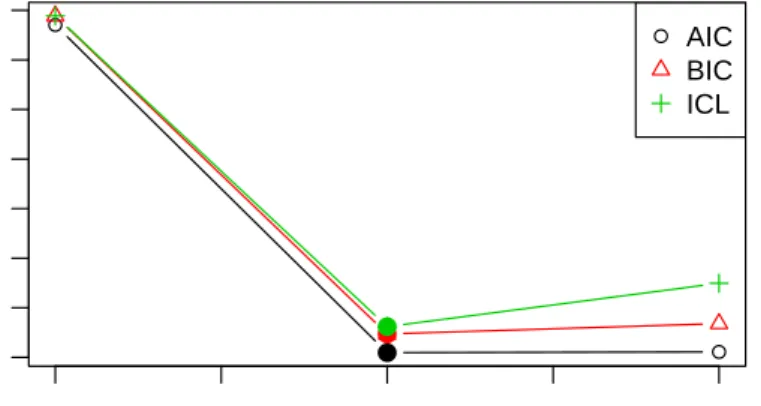
To inspect the results, the returned object can either be printed, as illustrated above, or plotted yielding a visualization of information criteria (see Figure 1). Both printed display and visualization show a big difference in information criteria across numer of componentsK, with the minimum always being assumed for K= 2, thus correctly recovering the two latent classes constructed in the underlying DGP.
The values of the information criteria can also be accessed directly via the functions of the cor-responding names. To select a certain model from a “stepRaschmix” object, thegetModel()
function from the flexmix package can be employed. The specification of whichmodel is to be selected can either be an information criterion, or the number of components as a string, or the index of the model in the original vector k. In this particular case, which = "BIC",
which = "2", and which = 2would all return the model with K= 2 components.
R> BIC(m1)
1 2 3
20944.07 17736.04 17840.42
R> m1b <- getModel(m1, which = "BIC") R> summary(m1b)
● ● ● 1.0 1.5 2.0 2.5 3.0 17500 19000 20500 number of components ● AIC BIC ICL ● ● ●
Figure 1: Information criteria for Rost’s model withK = 1,2,3 components for the artifical scenario 2 data.
Call:
raschmix(formula = r2, k = 2) prior size post>0 ratio
Comp.1 0.498 808 1262 0.640 Comp.2 0.502 820 1264 0.649 Item Parameters: Comp.1 Comp.2 Item01 -2.5574826 2.4538561 Item02 -2.1844001 2.1573277 Item03 -1.4524543 1.6382597 Item04 -1.0042438 0.9254200 Item05 -0.3639643 0.2675059 Item06 0.3074967 -0.3868124 Item07 0.8828234 -0.8563867 Item08 1.5048074 -1.4900729 Item09 2.1186345 -2.0921240 Item10 2.7487831 -2.6169734 'log Lik.' -8738.606 (df=35) AIC: 17547.21 BIC: 17736.04
To inspect the main properties of the model,summary()can be called. The information about the components of the mixture includes a priori component weights πk and sizes as well as
the information criteria AIC and BIC are reported. As one of the item parameters in the Rasch model is not identified, a restriction needs to be applied to the item parameters. In the output of thesummary() function, the item parameters of each component are scaled to sum to zero.
Two other functions, worth()andparameters(), can be used to access the item parameters. The sum restriction employed in the summary() output is also applied by worth(). Addi-tionally, worth() provides the possibilities to select several or just one specific component
and to transform item difficulty parameters to item easiness parameters. The function
parameters() also offers these two options but restricts the first item parameter to be zero
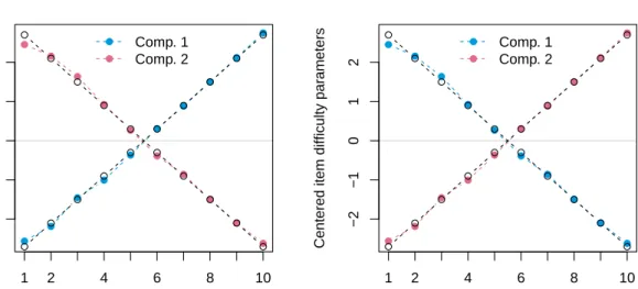
(rather than the sum of item parameters), as this restriction is used in the internal com-putations. Thus, for the illustrative dataset with 10 items, parameters() returns 9 item parameters, leaving out the first item parameter restricted to zero while worth() returns 10 item parameters summing to zero. The latter corresponds to the parametrization employed by Rost (1990) and simRaschmix(). For convenience reasons, the true parameters are at-tached to the simulated dataset as an attribute named"item". These are printed below and visualized in Figure2(left), showing that all item parameters are recovered rather well. Note that the ordering of the components in mixture models is generally arbitrary.
R> parameters(m1b, "item") Comp.1 Comp.2 item.Item02 0.3730825 -0.2965283 item.Item03 1.1050282 -0.8155963 item.Item04 1.5532388 -1.5284360 item.Item05 2.1935182 -2.1863502 item.Item06 2.8649793 -2.8406685 item.Item07 3.4403060 -3.3102427 item.Item08 4.0622900 -3.9439290 item.Item09 4.6761171 -4.5459800 item.Item10 5.3062656 -5.0708294 R> worth(m1b) Comp.1 Comp.2 Item01 -2.5574826 2.4538561 Item02 -2.1844001 2.1573277 Item03 -1.4524543 1.6382597 Item04 -1.0042438 0.9254200 Item05 -0.3639643 0.2675059 Item06 0.3074967 -0.3868124 Item07 0.8828234 -0.8563867 Item08 1.5048074 -1.4900729 Item09 2.1186345 -2.0921240 Item10 2.7487831 -2.6169734 R> attr(r2, "item")
beta1 beta2 1 2.7 -2.7 2 2.1 -2.1 3 1.5 -1.5 4 0.9 -0.9 5 0.3 -0.3 6 -0.3 0.3 7 -0.9 0.9 8 -1.5 1.5 9 -2.1 2.1 10 -2.7 2.7
In addition to the item parameters, theparameters()function can also return the parameters of the "score" model and the "concomitant" model (if any). The type of parameters can be set via the which argument. Per default parameters() returns both item and score parameters.
A comparison between estimated and true class membership can be conducted using the
clusters() function and the corresponding attribute of the data, respectively. As already
noticeable from the item parameters, the first component of the mixture matches the second true group of the data and vice versa. This label-switching property of mixture models in general can also be seen in the cross-table of class memberships. We thus have 38 misclassi-fications among the 1628 observations.
R> table(model = clusters(m1b), true = attr(r2, "group"))
true
model 1 2
1 16 792
2 798 22
For comparison, a Rasch mixture model with mean/variance parametrization for the score probabilites, as introduced in Section2.3, is fitted with one to three components and the best BIC model is selected.
R> m2 <- raschmix(data = r2, k = 1:3, scores = "meanvar")
R> m2
Call:
raschmix(data = r2, k = 1:3, scores = "meanvar")
iter converged k k0 logLik AIC BIC ICL
1 2 TRUE 1 1 -10416.199 20854.40 20913.74 20913.74
2 8 TRUE 2 2 -8747.084 17540.17 17664.25 17737.65
3 60 TRUE 3 3 -8738.314 17546.63 17735.46 17939.80
Items
Centered item difficulty par
ameters −2 −1 0 1 2 ● ● ● ● ● ● ● ● ● ● ● ● ● ● ● ● ● ● ● ● 1 2 4 6 8 10 ● ● Comp. 1 Comp. 2 ● ● ● ● ● ● ● ● ● ● ● ● ● ● ● ● ● ● ● ● Items
Centered item difficulty par
ameters −2 −1 0 1 2 ● ● ● ● ● ● ● ● ● ● ● ● ● ● ● ● ● ● ● ● 1 2 4 6 8 10 ● ● Comp. 1 Comp. 2 ● ● ● ● ● ● ● ● ● ● ● ● ● ● ● ● ● ● ● ●
Figure 2: True (black) and estimated (blue/red) item parameters for the two model specifi-cations,"saturated"(left) and"meanvar" (right), for the artifical scenario 2 data.
As in the saturated version of the Rasch mixture model, all three information criteria prefer the two-component model. Thus, this version of a Rasch mixture model is also capable of recognizing the two latent classes in the data while using a more parsimonious parametrization with 23 instead of 35 parameters.
R> logLik(m2b)
'log Lik.' -8747.084 (df=23)
R> logLik(m1b)
'log Lik.' -8738.606 (df=35)
The estimated parameters of the distribution of the score probabililities can be accessed through parameters() while the full set of score probabilities is returned by scoreProbs(). The estimated score probabilites of the illustrative model are approximately equal across components and roughly uniform.
R> parameters(m2b, which = "score")
Comp.1 Comp.2
score.location -0.10292905 -0.04187548
score.dispersion -0.09456975 -0.07905495
Comp.1 Comp.2 0 0.0000000 0.0000000 1 0.1198694 0.1163454 2 0.1155415 0.1133228 3 0.1122157 0.1110791 4 0.1098133 0.1095705 5 0.1082785 0.1087681 6 0.1075758 0.1086567 7 0.1076895 0.1092340 8 0.1086219 0.1105110 9 0.1103944 0.1125124 10 0.0000000 0.0000000
The resulting item parameters for this particular data set are virtually identical to those from the saturated version, as can be seen in Figure2.
To demonstrate the use of a concomitant variable model for the weights of the mixture, the two artificial variablesx1and x2are employed. They are added on the right-hand side of the formula, yielding a multinomial logit model for the weights (only ifk = 2or more components are specified).
R> cm2 <- raschmix(resp ~ x1 + x2, data = d, k = 2:3, scores = "meanvar")
The BIC is used to compare the models with and without concomitant variables. In both cases, the two true groups are recognized correctly, while the model with concomitants manages to employ the additional information and reaches a somewhat improved model fit.
R> rbind(m2 = BIC(m2), cm2 = c(NA, BIC(cm2)))
1 2 3
m2 20913.74 17664.25 17735.46
cm2 NA 17611.05 17691.59
As mentioned above, the parameters of the concomitant model can be accessed via the
parameters() function, setting which = "concomitant". The influence of the informative
covariatex1is reflected in the large absolute coefficient while the estimated coefficient for the noninformative covariatex2is close to zero.
R> cm2b <- getModel(cm2, which = "BIC") R> parameters(cm2b, which = "concomitant")
1 2
(Intercept) 0 0.43688740
x1 0 -0.85033332
x2 0 0.03043432
The corresponding estimated item parametersparameters(cm2b, "item")are not very dif-ferent from the previous models (and are hence not shown here). This illustrative application
shows that the inclusion of concomitant variables can provide additional information, e.g., thatx1 but notx2is associated with the class membership. Note also that this is picked up although a rather weak association was simulated here.
R> table(x1 = d$x1, clusters = clusters(cm2b))
clusters
x1 1 2
0 320 494 1 486 328
4. Empirical application: Verbal aggression
The verbal aggression dataset (De Boeck and Wilson 2004) contains item response data from 316 first-year psychology students along with gender and trait anger (assessed by the Dutch adaptation of the state-trait anger scale) as covariates (Smits, De Boeck, and Vansteelandt 2004). The 243 women and 73 men responded to 24 items constructed the following way: Following the description of a frustrating situation, subjects are asked to agree or disagree with a possible reaction. The situations are described by the following four sentences:
S1: A bus fails to stop for me.
S2: I miss a train because a clerk gave me faulty information.
S3: The grocery store closes just as I am about to enter.
S4: The operator disconnects me when I had used up my last 10 cents for a call. Each reaction begins with either “I want to” or “I do” and is followed by one of the three verbally aggressive reactions “curse”, “scold”, or “shout”, e.g., “I want to curse”, “I do curse”, “I want to scold”, or “I do scold”.
For our illustration, we use only the first two sentences which describe situations in which the others are to blame. Extreme-scoring subjects agreeing with either none or all responses are removed.
R> data("VerbalAggression", package = "psychotools")
R> VerbalAggression$resp2 <- VerbalAggression$resp2[, 1:12] R> va12 <- subset(VerbalAggression,
+ rowSums(resp2) > 0 & rowSums(resp2) < 12) R> colnames(va12$resp2)
[1] "S1WantCurse" "S1DoCurse" "S1WantScold" "S1DoScold"
[5] "S1WantShout" "S1DoShout" "S2WantCurse" "S2DoCurse"
[9] "S2WantScold" "S2DoScold" "S2WantShout" "S2DoShout"
We fit Rasch mixture models with the mean/variance score model, one to four components, and with and without the two concomitant variables, respectively (the single component model being only fitted without covariates).
Rootogram of posterior probabilities > 1e−04 0 50 100 0.0 0.2 0.4 0.6 0.8 1.0 Comp. 1 0.0 0.2 0.4 0.6 0.8 1.0 Comp. 2 0.0 0.2 0.4 0.6 0.8 1.0 Comp. 3
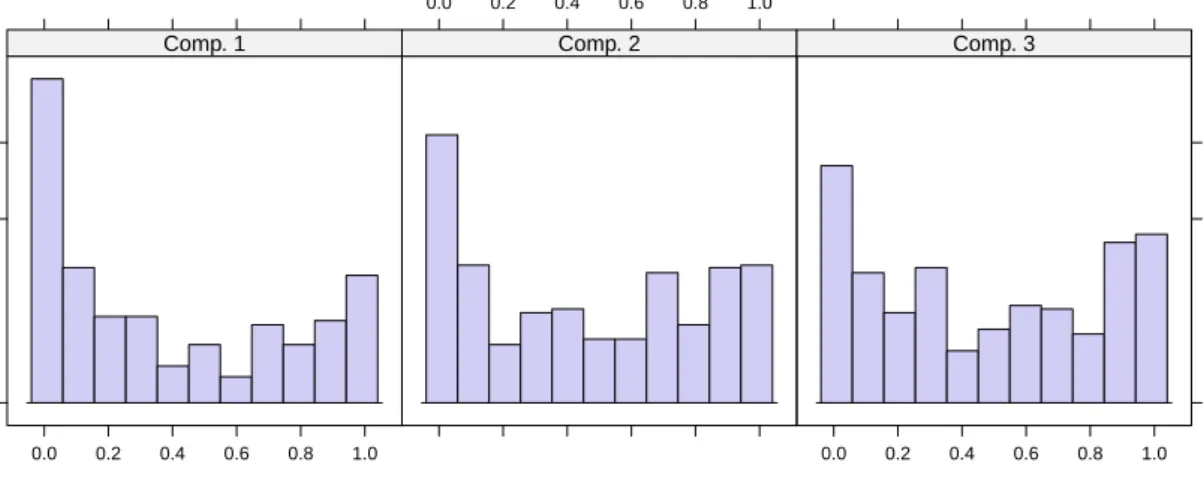
Figure 3: Rootogram of posterior probabilties in the 3-component Rasch mixture model on verbal aggression data.
R> set.seed(1)
R> va12_mix1 <- raschmix(resp2 ~ 1, data = va12, k = 1:4, scores = "meanvar") R> va12_mix2 <- raschmix(resp2 ~ gender + anger, data = va12, k = 2:4,
+ scores = "meanvar")
The correspondig BIC for all considered models can be computed by
R> rbind(BIC(va12_mix1), c(NA, BIC(va12_mix2)))
1 2 3 4
[1,] 3874.632 3857.567 3854.350 3887.361
[2,] NA 3859.119 3854.822 3880.484
R> va12_mix3 <- getModel(va12_mix1, which = "3")
showing that three components are preferred regardless of whether or not concomitant vari-ables are used. In this case, they do not lead to a better model fit, thus the 3-class model without concomitant variables is chosen.
The posterior probabilities for the three components can be visualized via
histogram(va12_mix3)– by default using a square-root scale, yielding a so-called rootogram
– as shown in Figure 3. In the ideal case, posterior probilities of the observations for each component are either high or low, yielding a U-shape in all panels. In this case here, the components are separated acceptably well.
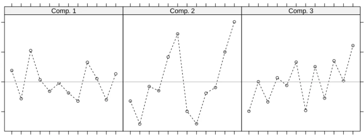
The item profiles in three components can be visualized via plot(va12_mix3) or
xyplot(va12_mix3) with the output of the latter being shown in Figure 4. The first six
items are responses to the first sentence (bus), the remaining six refer to the second sentence (train). The six reactions are grouped in “want”/“do” pairs: first for “curse”, then “scold”, and finally “shout”.
Item
Centered item difficulty par
ameters −2 0 2 4 1 2 3 4 5 6 7 8 9 10 11 12 ● ● ● ● ● ● ● ● ● ● ● ● Comp. 1 1 2 3 4 5 6 7 8 9 10 11 12 ● ● ● ● ● ● ● ● ● ● ● ● Comp. 2 1 2 3 4 5 6 7 8 9 10 11 12 ● ● ● ● ● ● ● ● ● ● ● ● Comp. 3
Figure 4: Item profiles for the 3-component Rasch mixture model on verbal agression data. Items 1–6 pertain to situation S1 (bus), items 7–12 to situation S2 (train), each in the following order: want to curse, do curse, want to scold, do scold, want to shout, do shout.
The third component displays a zigzag pattern which indicates that subjects in this component always find it easier or less extreme to “want to” react a certain way rather than to actually “do” react that way. In the other two components this want/do relationship is reversed, except
for the shouting response (to either situation).
In the first component, there are no big differences in the estimated item parameters. Neither the situation (S1 or S2) nor the type of verbal response (curse, scold, or shout) is particularly hard to agree to for subjects in this component. In components 2 and 3, the situation is also not very relevant but subjects differentiate between the three verbal responses. This is best visible in component 2 where item difficulty is clearly increasing from response “curse” to response “shout”. Thus, shouting is preceived as the most extreme verbal response while cursing is considered a comparably moderate response. In component 3 this pattern is also visible albeit not as prominently as in component 2.
One could also consider the 3-component model with concomitant variables as its BIC was almost equivalent to that of the model without concomitant variables. The estimated item parameters are virtually identical between both models and are hence not shown here. Nev-ertheless, the link between the concomitant variables and the latent classes may still be of interest:
R> parameters(getModel(va12_mix2, which = "3"), which = "concomitant")
1 2 3
(Intercept) 0 -0.76040110 -3.6721134
gendermale 0 1.66471685 1.4177908
anger 0 0.01155322 0.1268023
The absolute sizes of the cofficients reflect that there may be some association with gender but less with the anger score. However, as there is a slight increase in BIC compared to the model
without concomitants, the association with the covariates appears to be relatively weak. In comparison to other approaches exploring the association of class membership with covariates ex post (e.g., as in Cohen and Bolt 2005), the main advantage of the concomitant variables model lies in thesimulataneous estimation of the mixture and the influence of covariates.
5. Summary
Mixtures of Rasch models are a flexible means of checking measurement invariance and testing for differential item functioning. Here, we establish a rather general unifying conceptual framework for Rasch mixture models along with the corresponding computational tools in theRpackagepsychomix. In particular, this includes the original model specification ofRost
(1990) as well as more parsimoneous parameterizations (Rost and von Davier 1995), along with the possibility to incorporate concomitant variables predicting the latent classes (as in
Tayet al. 2011).
The R implementation is based on the infrastructure provided by the flexmix package, al-lowing for convenient model specification and selection. The rich set of methods forflexmix objects is complemented by additional functions specifically designed for Rasch models, e.g., extracting different types of parameters in different transformations and visualizing the esti-mated component-specific item parameters in various ways. Optionally, speed gains can be obtained from utilizing theC++ implementation in the mRm package for selecting optimal starting values. Thus, psychomix provides a comprehensive and convenient toolbox for the application of Rasch mixture models in psychometric research practice.
Acknowledgments
We are thankful to the participants of the “Psychoco 2011” workshop at Universit¨at T¨ubingen for helpful feedback and discussions.
References
Ackerman TA (1992). “A Didactic Explanation of Item Bias, Item Impact, and Item Validity From a Multidimensional Perspective.”Journal of Educational Measurement,29(1), 67–91. Andersen EB (1972). “A Goodness of Fit Test for the Rasch Model.” Psychometrika,38(1),
123–140.
Cohen AS, Bolt DM (2005). “A Mixture Model Analysis of Differential Item Functioning.” Journal of Educational Measurement,42(2), 133–148.
Dayton CM, Macready G (1988). “Concomitant-Variable Latent-Class Models.” Journal of the American Statistical Association,83(401), 173–178.
De Boeck P, Wilson M (eds.) (2004). Explanatory Item Response Models: A Generalized Linear and Nonlinear Approach. Springer-Verlag, New York.
Dempster A, Laird N, Rubin D (1977). “Maximum Likelihood from Incomplete Data via the EM Algorithm.” Journal of the Royal Statistical Society B,39(1), 1–38.
Fischer GH, Molenaar IW (eds.) (1995). Rasch Models: Foundations, Recent Developments, and Applications. Springer-Verlag, New York.
Gr¨un B, Leisch F (2008). “FlexMix Version 2: Finite Mixtures with Concomitant Variables and Varying and Constant Parameters.”Journal of Statistical Software,28(4), 1–35. URL http://www.jstatsoft.org/v28/i04/.
Leisch F (2004). “FlexMix: A General Framework for Finite Mixture Models and Latent Class Regression in R.” Journal of Statistical Software, 11(8), 1–18. URL http://www. jstatsoft.org/v11/i08/.
Mair P, Hatzinger R (2007). “Extended Rasch Modeling: The eRm Package for the Ap-plication of IRT Models in R.” Journal of Statistical Software, 20(9), 1–20. URL http://www.jstatsoft.org/v20/i09/.
Preinerstorfer D (2011). mRm: AnRPackage for Conditional Maximum Likelihood Estima-tion in Mixed Rasch Models. R package version 1.0, URLhttp://CRAN.R-project.org/ package=mRm.
Rasch G (1960). Probabilistic Models for Some Intelligence and Attainment Tests. The University of Chicago Press.
RDevelopment Core Team (2011).R: A Language and Environment for Statistical Computing.
RFoundation for Statistical Computing, Vienna, Austria. ISBN 3-900051-07-0, URLhttp: //www.R-project.org/.
Rizopoulos D (2006). “ltm: An R Package for Latent Variable Modeling and Item Re-sponse Theory Analyses.” Journal of Statistical Software, 17(5), 1–25. URL http: //www.jstatsoft.org/v17/i05/.
Rost J (1990). “Rasch Models in Latent Classes: An Integration of Two Approaches to Item Analysis.”Applied Psychological Measurement,14(3), 271–282.
Rost J, von Davier M (1995). “Mixture Distribution Rasch Models.” In GH Fischer, IW Mole-naar (eds.), Rasch Models: Foundations, Recent Developments, and Applications, chap-ter 14, pp. 257–268. Springer-Verlag, New York.
Smits DJM, De Boeck P, Vansteelandt K (2004). “The Inhibition of Verbally Aggressive Behaviour.”European Journal of Personality,18(7), 537–555.
Strobl C, Kopf J, Zeileis A (2011). “A New Method for Detecting Differential Item Functioning in the Rasch Model.”Working Paper 2011-01, Working Papers in Economics and Statistics, Research Platform Empirical and Experimental Economics, Universit¨at Innsbruck. URL http://EconPapers.RePEc.org/RePEc:inn:wpaper:2011-01.
Tay L, Newman DA, Vermunt JK (2011). “Using Mixed-Measurement Item Response The-ory with Covariates (MM-IRT-C) to Ascertain Observed and Unobserved Measurement Equivalence.”Organizational Research Methods,14(1), 147–176.
Van den Noortgate W, De Boeck P (2005). “Assessing and Explaining Differential Item Func-tioning Using Logistic Mixed Models.” Journal of Educational and Behavioral Statistics, 30(4), 443–464.
Zeileis A, Strobl C, Wickelmaier F (2011). psychotools: Infrastructure for Psychome-tric Modeling. R package version 0.1-1, URL http://CRAN.R-project.org/package= psychotools.
Affiliation:
Hannah Frick, Achim Zeileis Department of Statistics Universit¨at Innsbruck Universit¨atsstr. 15 6020 Innsbruck, Austria
E-mail: [email protected],[email protected]
URL: http://eeecon.uibk.ac.at/~frick/,http://eeecon.uibk.ac.at/~zeileis/ Carolin Strobl Department of Psychology Universit¨at Z¨urich Binzm¨uhlestr. 14 8050 Z¨urich, Switzerland E-mail: [email protected] URL: http://www.psychologie.uzh.ch/fachrichtungen/methoden.html Friedrich Leisch
Institute of Applied Statistics and Computing Universit¨at f¨ur Bodenkultur Wien
Peter Jordan-Str. 82 1180 Wien, Austria
E-mail: [email protected]
http://eeecon.uibk.ac.at/wopec/
2011-21 Hannah Frick, Carolin Strobl, Friedrich Leisch, Achim Zeileis: Flexi-ble Rasch mixture models with package psychomix
2011-20 Thomas Grubinger, Achim Zeileis, Karl-Peter Pfeiffer: evtree: Evolu-tionary learning of globally optimal classification and regression trees in R
2011-19 Wolfgang Rinnergschwentner, Gottfried Tappeiner, Janette Walde: Multivariate stochastic volatility via wishart processes - A continuation
2011-18 Jan Verbesselt, Achim Zeileis, Martin Herold: Near Real-Time Distur-bance Detection in Terrestrial Ecosystems Using Satellite Image Time Series: Drought Detection in Somalia
2011-17 Stefan Borsky, Andrea Leiter, Michael Pfaffermayr: Does going green pay off? The effect of an international environmental agreement on tropical timber trade
2011-16 Pavlo Blavatskyy: Stronger Utility
2011-15 Anita Gantner, Wolfgang H¨ochtl, Rupert Sausgruber:The pivotal me-chanism revisited: Some evidence on group manipulation
2011-14 David J. Cooper, Matthias Sutter: Role selection and team performance
2011-13 Wolfgang H¨ochtl, Rupert Sausgruber, Jean-Robert Tyran:Inequality aversion and voting on redistribution
2011-12 Thomas Windberger, Achim Zeileis: Structural breaks in inflation dyna-mics within the European Monetary Union
2011-11 Loukas Balafoutas, Adrian Beck, Rudolf Kerschbamer, Matthias Sutter: What drives taxi drivers? A field experiment on fraud in a market for credence goods
2011-10 Stefan Borsky, Paul A. Raschky: A spatial econometric analysis of com-pliance with an international environmental agreement on open access re-sources
2011-09 Edgar C. Merkle, Achim Zeileis: Generalized measurement invariance tests with application to factor analysis
American Economic Review
2011-07 Ernst Fehr, Daniela R¨utzler, Matthias Sutter:The development of ega-litarianism, altruism, spite and parochialism in childhood and adolescence
2011-06 Octavio Fern´andez-Amador, Martin G¨achter, Martin Larch, Georg Peter: Monetary policy and its impact on stock market liquidity: Evidence from the euro zone
2011-05 Martin G¨achter, Peter Schwazer, Engelbert Theurl: Entry and exit of physicians in a two-tiered public/private health care system
2011-04 Loukas Balafoutas, Rudolf Kerschbamer, Matthias Sutter: Distribu-tional preferences and competitive behavior forthcoming in
Journal of Economic Behavior and Organization
2011-03 Francesco Feri, Alessandro Innocenti, Paolo Pin:Psychological pressure in competitive environments: Evidence from a randomized natural experiment: Comment
2011-02 Christian Kleiber, Achim Zeileis: Reproducible Econometric Simulations
2011-01 Carolin Strobl, Julia Kopf, Achim Zeileis: A new method for detecting differential item functioning in the Rasch model
2010-29 Matthias Sutter, Martin G. Kocher, Daniela R¨utzler and Stefan T. Trautmann: Impatience and uncertainty: Experimental decisions predict adolescents’ field behavior
2010-28 Peter Martinsson, Katarina Nordblom, Daniela R¨utzler and Matt-hias Sutter: Social preferences during childhood and the role of gender and age - An experiment in Austria and Sweden Revised version forthcoming in Economics Letters
2010-27 Francesco Feri and Anita Gantner: Baragining or searching for a better price? - An experimental study. Revised version accepted for publication in Games and Economic Behavior
2010-26 Loukas Balafoutas, Martin G. Kocher, Louis Putterman and Matt-hias Sutter: Equality, equity and incentives: An experiment
2010-25 Jes´us Crespo-Cuaresma and Octavio Fern´andez Amador: Business cycle convergence in EMU: A second look at the second moment
2010-24 Lorenz Goette, David Huffman, Stephan Meier and Matthias Sutter: Group membership, competition and altruistic versus antisocial punishment: Evidence from randomly assigned army groups
2010-22 Jes´us Crespo-Cuaresma and Octavio Fern´andez Amador: Buiness cycle convergence in the EMU: A first look at the second moment
2010-21 Octavio Fern´andez-Amador, Josef Baumgartner and Jes´us Crespo-Cuaresma: Milking the prices: The role of asymmetries in the price trans-mission mechanism for milk products in Austria
2010-20 Fredrik Carlsson, Haoran He, Peter Martinsson, Ping Qin and Matt-hias Sutter: Household decision making in rural China: Using experiments to estimate the influences of spouses
2010-19 Wolfgang Brunauer, Stefan Lang and Nikolaus Umlauf:Modeling hou-se prices using multilevel structured additive regression
2010-18 Martin G¨achter and Engelbert Theurl:Socioeconomic environment and mortality: A two-level decomposition by sex and cause of death
2010-17 Boris Maciejovsky, Matthias Sutter, David V. Budescu and Patrick Bernau: Teams make you smarter: Learning and knowledge transfer in auc-tions and markets by teams and individuals
2010-16 Martin G¨achter, Peter Schwazer and Engelbert Theurl: Stronger sex but earlier death: A multi-level socioeconomic analysis of gender differences in mortality in Austria
2010-15 Simon Czermak, Francesco Feri, Daniela R¨utzler and Matthias Sut-ter:Strategic sophistication of adolescents - Evidence from experimental normal-form games
2010-14 Matthias Sutter and Daniela R¨utzler: Gender differences in competition emerge early in live
2010-13 Matthias Sutter, Francesco Feri, Martin G. Kocher, Peter Martins-son, Katarina Nordblom and Daniela R¨utzler: Social preferences in childhood and adolescence - A large-scale experiment
2010-12 Loukas Balafoutas and Matthias Sutter: Gender, competition and the efficiency of policy interventions
2010-11 Alexander Strasak, Nikolaus Umlauf, Ruth Pfeifer and Stefan Lang: Comparing penalized splines and fractional polynomials for flexible modeling of the effects of continuous predictor variables
2010-10 Wolfgang A. Brunauer, Sebastian Keiler and Stefan Lang: Trading strategies and trading profits in experimental asset markets with cumulative information
2010-08 Martin G. Kocher, Marc V. Lenz and Matthias Sutter: Psychological pressure in competitive environments: Evidence from a randomized natural experiment: Comment
2010-07 Michael Hanke and Michael Kirchler: Football Championships and Jer-sey sponsors’ stock prices: An empirical investigation
2010-06 Adrian Beck, Rudolf Kerschbamer, Jianying Qiu and Matthias Sut-ter: Guilt from promisebreaking and trust in markets for expert services -Theory and experiment
2010-05 Martin G¨achter, David A. Savage and Benno Torgler: Retaining the thin blue line: What shapes workers’ intentions not to quit the current work environment
2010-04 Martin G¨achter, David A. Savage and Benno Torgler:The relationship between stress, strain and social capital
2010-03 Paul A. Raschky, Reimund Schwarze, Manijeh Schwindt and Fer-dinand Zahn: Uncertainty of governmental relief and the crowding out of insurance
2010-02 Matthias Sutter, Simon Czermak and Francesco Feri: Strategic sophi-stication of individuals and teams in experimental normal-form games
2010-01 Stefan Lang and Nikolaus Umlauf: Applications of multilevel structured additive regression models to insurance data
Working Papers in Economics and Statistics
2011-21
Hannah Frick, Carolin Strobl, Friedrich Leisch, Achim Zeileis Flexible Rasch mixture models with package psychomix
Abstract
Measurement invariance is an important assumption in the Rasch model and mixture models constitute a flexible way of checking for a violation of this assumption by detecting unobserved heterogeneity in item response data. Here, a general class of Rasch mixture models is established and implemented in R, using conditional maximum likelihood estimation of the item parameters (given the raw scores) along with flexible specification of two model building blocks: (1) Mixture weights for the unobserved classes can be treated as model parameters or based on covariates in a concomitant variable model. (2) The distribution of raw score probabilities can be parametrized in two possible ways, either using a saturated model or a specification through mean and variance. The function raschmix() in the R package ”psychomix”provides these models, leveraging the general infrastructure for fitting mixture models in the ”flexmix”package. Usage of the function and its associated methods is illustrated on artificial data as well as empirical data from a study of verbally aggressive behavior.
ISSN 1993-4378 (Print) ISSN 1993-6885 (Online)