Directly Learning Tractable Models for Sequential Inference and DecisionMaking

(1)

Directly Learning Tractable Models for

Sequential Inference and Decision Making

by

Mazen Melibari

A thesis

presented to the University of Waterloo in fulfillment of the

thesis requirement for the degree of Doctor of Philosophy

in

Computer Science

Waterloo, Ontario, Canada, 2016 © Mazen Melibari 2016

(2)

any required final revisions, as accepted by my examiners.

(3)

Abstract

Probabilistic graphical models such as Bayesian networks and Markov networks provide a general framework to represent multivariate distributions while exploiting conditional indepen-dence. Over the years, many approaches have been proposed to learn the structure of those networks Heckerman et al. (1995); Neapolitan (2004). However, even if the resulting network is small, inference may be intractable (e.g., exponential in the size of the network) and practi-tioners must often resort to approximate inference techniques. Recent work has focused on the development of alternative graphical models such as arithmetic circuits (ACs) Darwiche (2003) and sum-product networks (SPNs) Poon and Domingos (2011) for which inference is guaranteed to be tractable (e.g., linear in the size of the network for SPNs and ACs). This means that the networks learned from data can be directly used for inference without any further approxima-tion. So far, previous work has focused on learning models with only random variables and for a fixed number of variables based on fixed-length data Lowd and Domingos (2012); Dennis and Ventura (2012); Gens and Domingos (2013); Peharz et al. (2013); Rooshenas and Lowd (2014). In this thesis, I present two new probabilistic graphical models: Dynamic Sum-Product Networks (DynamicSPNs) and Decision Sum-Product-Max Networks (DecisionSPMNs), where the for-mer is suitable for problems with sequence data of varying length and the latter is for problems with random, decision, and utility variables. Similar to SPNs and ACs,DynamicSPNs and De-cisionSPMNs can be learned directly from data with guaranteed tractable exact inference and decision making in the resulting models. I also present a new online Bayesian discriminative learning algorithm for Selective Sum-Product Networks (SSPNs), which are a special class of SPNs with no latent variables. This new learning algorithm achieves tractability by utilizing a novel idea ofmode matching, where the algorithm chooses a tractable distribution that matches the mode of the exact posterior after processing each training instance. This approach lends it-self naturally to distributed learning since the data can be divided into subsets based on which

(4)

Words cannot express how grateful I am to all the people who made this thesis possible. My deepest appreciation goes to my supervisor, Prof. Pascal Poupart, whose expertise and patience aided me considerably during my PhD journey. I would also like to express my sincere appreciation for my co-supervisor, Prof. Ed-ward Lank, for his support and encouragement. I have been extremely fortunate to have Prof. Poupart and Prof Lank as my supervisors, and without them, I could not have finished this thesis.

I am grateful to Prof. Prashant Doshi for the amazing collaboration, which be-came one of the chapters in this thesis. I am indebted to him for his insightful comments, long discussions, and practical advices.

I am also thankful for all my friends who made this journey much more enjoyable and helped me through difficult times. My special thanks go to Akram Nour, Zuhair Milibari, Ahmad Basalah, Badr Lami, Omar Almahdi, Ayman Alharbi, Han Zhao, Hadi Hosseini, Shehroz Khan, Abdullah Rashwan, and Igor Kiselev for their endless help and support during my PhD journey.

Finally, I want to express my sincere appreciation for my parents and my lovely wife, Nujud. Thank you for all the sacrifices you made to help me to complete this PhD. Nothing I could ever do would repay you for all you have done for me. Without your love and support, this thesis would not have happened.

(5)

Dedication

To my father, for being so generous .. To my mother, for her loving heart .. To my lovely wife, for being beside me ..

(6)

List of Tables

3.1 Mean negative log-likelihood and standard error based on 10-fold cross validation for the synthetic datasets. (#i,length,#oVars) indicates the number of data instances, length of each sequence and number of observed variables. Lower likelihoods are better. . . 45 3.2 Mean negative log-likelihood and standard error based on 10-fold cross validation

for the real world datasets. (#i,length,#oVars) indicates the number of data instances, average length of the sequences and number of observed variables. . . 45 3.3 Comparisons of the learning and inference times of the networks learned by Reveal,

RNN, Search-Score DBN (SS DBN) and DSPN. . . 46 4.1 Statistics of the datasets used in the experiments. . . 62 5.1 Problem, datasets, and learned models statstics. #Dec var is the number of

deci-sions variables in the problem,|ID|is the total representational size of the influ-ence diagram (total clique size + sepsets),|Dataset|is the size of the dataset, and

(10)

The second and third columns are the MEU from the true model and Decision-SPMN, respectively. The optimal decision rule is obtained from the learned Deci-sionSPMNthen plugged into the true model; the resulting EU of the true model is shown in the fourth column. In the case where there is a discrepancy between theID’s MEU (second column) and EU (fourth column), then that means that the DecisionSPMN’s decision rule does not match the one from theID. In such cases, further analysis is performed to obtain the percentage of discrepancy, which is re-ported in the last column. MEU forDecisionSPMNis the mean of 10-fold cross-validation. The largest std. error across the folds among all the datasets was 0.00012. 79 5.3 Learning time forDecisionSPMNs in seconds and a comparison between the MEU

(11)

List of Figures

1.1 A Venn diagram shows the position of Sum-Product Networks within the space of possible functions and distributions. . . 4 2.1 Examples of Bayesian networks Pearl (1995); Koller and Friedman (2009). Each node

is associated with a random variable and a conditional probability distribution. (a) is the burglar alarm Bayesian network. (b) is known as the sprinkler network. . . . 15 2.2 Examples of two Markov network structures, (a) is an example of a Markov network

that encodes conditional independencies that can not be perfectly modeled using a Bayesian network (any Bayesian network will have either less or more conditional independence assertions); (b) is an example of a grid structure that is widely used in many computer vision and image processing applications Wang et al. (2013). . . . 16 2.3 An example Bayesian network withm+ 1variables. Each variable is represented by

a node in the graph and edges correspond to dependencies between the variables. This structure is also known as the Naive Bayes model. . . 17 2.4 The Bayesian network that is used in Example 2.3, (a) shows the structure of the

(12)

2.6 Basic distributions encoded as SPNs. (a) shows an SPN that encodes a univariate distribution over a binary variablex. (b) shows an SPN that encodes factored dis-tribution over three binary variablesx,y, andz. (c) is an SPN that encodes a naive Bayes model over three binary variablesx,y, andz. The root sum node corresponds to a the hidden class variable. . . 27 3.1 An example of a generic template network. Notice the interface nodes in red. . . . 32 3.2 A generic example of a completeDynamicSPNunrolled over 3 time slices.

Tem-plate network is stacked on the bottom network and capped by the top network. . 34 3.3 The SPN of the root product node in (a) is replaced by a product of naive Bayes

models in (b). . . 43 4.1 Experimental results of comparingDiscBaysto generative and (non-Bayesian)

dis-criminative learning algorithms. The X-axis shows the percentage of data used for training and the Y-axis shows the conditional log-likelihood of the testing dataset. 60 5.1 Example DecisionSPMN for one decision and one random variable. Notice the

rectangularmaxnode and the utility nodes (diamonds) in the leaves. . . 67 5.2 Similar to LearnSPN, LearnDecisionSPMN is a recursive algorithm that respects

the partial order and extends it to work with max and utility nodes. . . 72 5.3 An exampleDecisionSPMNlearned from the Computer Diagnostician dataset

us-ing LearnDecisionSPMN. The partial order used is{SysSt} ≺ RDecision ≺

{LogicF ail, IOF ail, ROutcome}. Three different indicators used for ROut-come because it is a ternary random variable. . . 73

(13)

List of Algorithms

2.1 Variable Elimination . . . 19

3.1 LearnDynamicSPN(): Anytime Search-and-Score Framework for DynamicSPNs 38 3.2 Initial Structure . . . 40

3.3 Neighbour . . . 42

3.4 GetPartition . . . 42

4.1 DiscBays(): An online Bayesian Discriminative Learning Algorithm for SSPNs 55 4.2 findMode() . . . 56

4.3 findHeight() . . . 58

4.4 modeMatching() . . . 58

5.1 LearnDecisionSPMN . . . 71

5.2 DecisionSPMNParameter Learning . . . 74

5.3 DecisionSPMNEM Up . . . 76

5.4 DecisionSPMNEM Down . . . 77

(14)

1 Introduction

Modeling and reasoning about uncertainty is at the heart of artificial intelligence (AI). Im-age understanding, speech recognition, robot navigation, and many other tasks in AI can be for-mulated as applications of modeling and reasoning about uncertainty. Uncertainty problems have different properties. For example, the variables of an uncertainty problem can be discrete or continuous, the number of variables can be fixed or dynamic, the relationships between the variables can be in one or two directions, and the variables can be fully or partially observed. These are a few examples of the variety of uncertainty problems. Through the history of AI, sev-eral frameworks have been proposed for modeling and reasoning about uncertainty Domingos (2006). One of the frameworks that proved to be general and suitable for the wide spectrum of uncertainty problems is the probabilistic graphical models (PGMs) framework. PGMs have many properties that make them among the elegant representational formalisms in AI. For one, they compactly represent probabilistic and decision problems. Consider for example a problem withnbinary random variables, the full specification of the joint distributions requiresO(2n)

(15)

able. PGMs also provide a declarative framework with clear semantics, which makes it easy to understand the relationship between the variables and grasp the decision making process in a decision problem. In addition to these, PGMs combine two heavily studied branches of mathe-matics: probability and graph theory, which together provide a sound machinery to reason and interpret the results in these models.

Although compactness, declarativity, and interpretability are appealing properties, what is more important in practice is the ability to answer queries about the uncertainty problem, which in the case of PGMs corresponds to performing inference to answer queries about some of the variables given the values of other variables. Unfortunately, when it comes to performing infer-ence PGMs generally suffer very badly from the curse of intractability. Exact inferinfer-ence in PGMs is known to be #P-Hard. Also, for many PGMs, existing inference algorithms are exponential in thetreewidthof the model’s structure, where the notion oftreewidthis a quantification of the structure resemblance to a tree. Thus, a practitioner who decides to use a PGM would often resort to either restrict himself to models with lowtreewidthor to use approximate inference, for which performance guarantees are also computationally hard to achieve (NP-hard) Dagum and Luby (1993).

There are several active lines of research that try to tackle the problem of tractable exact infer-ence in PGMs. They can, generally, be grouped into two categories. The first group contains the methods that restrict themselves within the space where exact inference is known to be tractable. This is, basically, the space of models that have low treewidth. Algorithms in this group include: Chow-Liu, Thin Junction Trees, and Bounded Treewidth. The main shortcoming of this type of algorithms is that focusing on only low treewidth models severely restricts the expressivity of the resulting models.

(16)

inference in PGMs can be seen as a sequence of sum and product operations. Therefore, the problem of tractable exact inference can be addressed by focusing on learning models that per-form these operations and making sure that the output of the models are correct answers of probabilistic queries that are of interest. Arithmetic Circuits (ACs) and Sum-Product Networks (SPNs) are examples of the models in this category. These two models are closely related. ACs were first proposed as inference machines in Darwiche (2003). The basic idea is that we can per-form inference on a PGM using one of the known inference algorithms and store the sequence of operations in a graph of sum and product nodes. This process is known in the literature as knowledge compilation. This work also introduces a concept of mathematical functions called network polynomialsthat encode probability distributions and can be evaluated to answer prob-abilistic queries.

Sum-Product Networks (SPNs) were proposed in Poon and Domingos (2011). SPNs are semantically equivalent to ACs. Poon and Domingos address two important issues. First, the process of knowledge compilation may blow up exponentially, because its complexity is equiva-lent to the complexity of the inference algorithm that is used in the compilation process. Second, knowledge compilation assumes the existence of a PGM before it starts the compilation process. Decomposability and smoothness are two properties that were originally proposed in Darwiche (2003) and reintroduced in Poon and Domingos (2011) under the name of decomposability and completeness. Poon and Domingo proved that SPNs encode proper joint distributions when they satisfy these two properties. Since SPNs and ACs are semantically equivalent, this result also applies to ACs. An SPN that encodes a proper joint distribution is called a valid SPN (or a valid AC, in the case of ACs). Exact inference in SPNs is always tractable and can be done in a

(17)

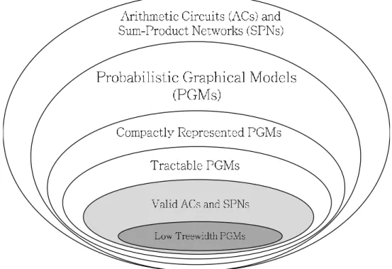
Figure 1.1 – A Venn diagram shows the position of Sum-Product Networks within the space of possible functions and distributions.

The Venn diagram in Figure 1.1 visualizes the relationship between ACs, SPNs, PGMs, com-pactly represented PGMs, tractable PGMs, valid ACs, valid SPNs, and low treewidth PGMs. Compactly represented PGMs are the family of PGMs where the representation size is polyno-mial in the number of variables. Tractable PGMs are the family of PGMs where the time of inference is polynomial in the number of variables. ACs and SPNs can be used to represent any arbitrary function; hence, the space of possible ACs and SPNs is a superset of the space of pos-sible PGMs. Most PGMs can be compactly represented, but only a subset of these are tractable. The notion of valid ACs and valid SPNs refers to subsets of ACs and SPNs that encode proper distributions. Since inference is tractable in low-treewidth PGMs, valid ACs and valid SPNs subsume this type of models and also include other type of PGMs where inference is tractable.

(18)

1.1 Uncertainty in Dynamic Settings

As mentioned above, uncertainty problems have different properties. One of the common properties of uncertainty problems is being dynamic. In a dynamic setting the number of vari-ables is not fixed and not known a priori. Consider for example a model that maps frames of YouTube videos to sequences of labels that describe the frames. Each frame can have a fixed number of variables that describe it (e.g., a variable for each pixel), but the number of frames varies from one YouTube video to another. Textual documents are usually treated as bags of words, but they can also be treated as sequences of words; also here the length of the sequence varies for each document.

A naive approach to deal with this problem is to define an upper bound for the number of variablesN, presumably based on the longest sequence that we have in a training set. Then, learn a fixed model with that number of variables. This approach suffers from two main problems. First, the resulting model will not be suitable for any sequence that is longer thanN. Second, if the sequences in the training set are mostly shorter thanN, we will end up having difficulties learning a correct model for the variables at the end, due to the shortage of data.

The previous approach completely ignores the dynamic nature of the problem and treats it as if it was a static problem. The other way to deal with this type of problems is to focus on captur-ing the dynamics of the problem, i.e., how the variables at each time step interact and how they affect the variables on the next time step. By focusing on these two things, we can effectively and compactly capture the dynamic nature of the problem. The type of PGMs that is designed for dynamic uncertainty problems is called Dynamic PGMs and they are usually defined by spec-ifying the interaction among the variables within each time step and between the time steps.

(19)

1.2. Uncertainty in Online Settings In this thesis, I present a new tractable probabilistic graphical model called Dynamic Sum-Product Networks (DynamicSPN) that tackles the intractability problem in Dynamic PGMs by directly learningtemplate SPNsthat effectively and compactly capture the dynamic nature of a problem from sequence data that can possibly be of varying length. As in the case of SPNs, exact inference inDynamicSPNs is always tractable and can be done in a time that is linear in the size of thetemplate SPNs. As part of theDynamicSPNs’ formulation, I introduced a new property, namedinvariance, that can be used to easily ensure that the DynamicSPNis valid (complete and decomposable). By exploiting this property, I also developed an iterative anytime search-and-score structure learning algorithm forDynamicSPNs that can learn the structure of a template SPN directly from data.

1.2 Uncertainty in Online Settings

Another common property of uncertainty problems that has been gaining even more popu-larity over the past several years is being online. In the online setting, the data is streamed into the model and the model has to update its belief incrementally. It is normal in this setting to assume that the model has only one chance to handle each data instance that appears in the stream. This means that many of the learning algorithms that perform multiple passes over the data during the learning process are not suitable for this type of settings. One paradigm that lends itself nat-urally to online settings is called Bayesian learning. It allows us to express prior knowledge about the model. Then, it updates the model after processing each data instance. Bayesian learning is mathematically elegant and very simple, but in most cases it is computationally hard.

Previous work A. Rashwan (2016) proposes the use of an approximation technique called moment matchingto develop a Bayesian learning algorithm for SPNs, where the focus was on

(20)

learning the joint distribution over random variables. This type of learning that focuses on the joint distribution is calledgenerative learning. In this thesis, I developed a new learning algorithm calledDiscBaysfor a special type of SPNs that has no latent variables.DiscBaysis an online algo-rithm that utilizes the Bayesian learning paradigm. It directly learns a conditional distribution of a target variable given another set of variables. This type of learning is known asdiscriminative learning. Unfortunately, themoment matching technique is not feasible in the discriminative case. Instead, I developed a novel approximation technique based on mode matching that and works nicely for the discriminative case.

1.3 Decision Making under Uncertainty

The notion ofintelligent agentsis yet another concept that is at the heart of AI. Agents are entities that have some perceptions about the environment and they can act upon it, where acting involves making decisions. Besides random variables, decision making problems often require two additional types of variables: decision and utility variables. Decision variables encode the possible actions an agent can take and utility variables encode the desirability of the possible outcomes. A main concern in AI is to develop what is known asrational agents. An agent is considered rational if it follows a set of axioms, namedaxioms of rationality; these axioms impose constraints on how to define the agent’s utility. A rational agent is also defined as an agent that follows themaximum expected utility principle, which states that the agent should always take the actions that maximize its expected utility. Influence diagrams (also known as decision networks) are a class of PGMs that concerns the problem of decision making under uncertainty. They provide a framework to define decision problems using three types of nodes: chance, decision, and utility nodes, where chance nodes correspond to random variables.

(21)

1.4. Summary of the Contributions This thesis presents a new model calledDecisionSPMN, which is an extension of SPNs to the class of decision making problems. To enable this, the new model introduces two new types of nodes:maxnodes to represent the maximization operation over different possible values of a decision variable, andutilitynodes to represent the utility values. The solution of a Decision-SPMNis the set of decisions that maximizes the expected utility and it can be computed in a time that is linear in the size of the network. The semantics of the max node is that its output is the value of the decision that leads to the maximal value among all decisions. Analogously to sum-product networks, I introduce a set of properties that guarantee the validity of the Deci-sionSPMN, such that the solution of aDecisionSPMNwill correspond to the expected utility obtained from a valid embedded probabilistic model and a utility function that are encoded by the network.

1.4 Summary of the Contributions

Using the idea of modeling inference, I developed two new probabilistic graphical models that guarantee tractable exact inference. I also developed a new online discriminative Bayesian parameter learning algorithm for a special class of tractable models called Selective Sum-Product Networks based on the novel idea of Bayesian mode matching. The following list summarizes the contributions made in this thesis:

• Dynamic Sum-Product Networks (DynamicSPNs):

I developed a new tractable exact inference model called: Dynamic Sum-Product Net-works (DynamicSPNs), that is suitable for sequence data of varying length. I introduced the concept of template networks that can be repeated to model data sequences of any

(22)

length. I also introduced a new property:invariance, which can be used to easily ensure that theDynamicSPNis valid (complete and decomposable)

• A Structure Learning Algorithm forDynamicSPNs (LearnDynamicSPN):

I developed an iterative anytime search-and-score structure learning algorithm for Dy-namicSPNs that can learn the structure of a template network directly from data. • A Discriminative Bayesian Learning Algorithm for Selective SPNs (DiscBays):

I developed a new online discriminative Bayesian learning technique for a special class of tractable models called Selective Sum-Product Networks based on the novel idea of Bayesian mode matching. This new technique can be used when data is presented in an online fashion and can easily be extended to a distributed learning setting.

• Decision Sum-Product Networks (DecisionSPMN):

I developed a new tractable model for decision problems, namedDecisionSPMN. This model adds two new types of nodes to SPNs: max nodes and utility nodes. Optimal de-cision strategies can be obtained fromDecisionSPMNin time that is linear in the size of the network.

• Structure and Parameter Learning forDecisionSPMNs (LearnDecisionSPMN):

I developed algorithms to learn both the structure and the parameters of decision prob-lems directly from data. The structure learning algorithm is recursive and respects the constraint imposed by the decision problem’s partial order.

(23)

1.5. Thesis Structure • Chapter 2

The background materials that are needed for the rest of the thesis are presented in this chapter. The chapter introduces two of the traditional probabilistic graphical models (PGMs): Bayesian networks and Markov networks. Then, after introducing the concept ofnetwork polynomialfunctions, the chapter explains SPNs, how to learn them, and how to do inference with them.

• Chapter 3

This chapter presents Dynamic Sum-Product Networks (DynamicSPNs). It also presents an invariance property that is sufficient to ensure that the resultingDynamicSPNis valid (i.e., encodes a joint distribution) by being complete and decomposable. The chapter also presents a general anytime search-and-score framework with a local search technique to learn the structure of a template network that defines aDynamicSPNbased on data se-quences of varying length. The experimental results section in this chapter demonstrates the advantages of DynamicSPNs over static SPNs, Dynamic Bayesian Networks, and Hidden Markov Models on synthetic and real sequence data.

• Chapter 4

This chapter presents a new online discriminative Bayesian learning algorithm called Dis-cBaysfor Selective Sum-Product Networks (SSPNs). After discussing SSPNs and the previous work on discriminative and Bayesian learning for SPNs, the chapter presents DiscBaysand provides a brief discussion of how to use it in a distributed fashion. The experimental section shows the results when comparingDiscBaysto generative and (non-Bayesian) discriminative learning algorithms.

(24)

The new tractable model for decision making,DecisionSPMN, is presented in this chap-ter. The chapter discuss the relationship betweenDecisionSPMNand some other related works. The formulation of DecisionSPMN along with the algorithms for learning the structure and the parameters are presented in this chapter.

• Chapter 6

This concluding chapter provides a summary of the thesis and a discussion of possible future directions.

(25)

Chapter

2 Background

This chapter starts by introducing two of the traditional probabilistic graphical models (PGMs): Bayesian networks and Markov networks. Section 2.2 explains how we can construct a function callednetwork polynomialthat encodes a joint distribution. Section 2.3 presents Sum-Product Networks (SPNs), which emerged recently as a new class of tractable probabilistic graphical mod-els, that are built upon the idea ofnetwork polynomialsand guarantee linear time inference in the size of the network.

2.1 Probabilistic Graphical Models

PGMs are a powerful and an elegant framework for modeling uncertainty by utilizing prob-ability theory and graph theory. Generally, a PGM G over a set of random variables X =

{X1, X2, ..., XN}is defined using a graphG = hV, Eiand a set of non-negative functions F, whereV is a set of nodes,Eis a set of edges such thatE ⊆V ×V; each noden ∈V is asso-ciated with a random variable. The set of functionsFfactorizes the joint distribution according

(26)

to the conditional independence constraints induced by the graphG. Gis called the structure of the PGM andFis its parameterization.

IfGis a directed acyclic graph (DAG), which means that all edges are directed and the graph contains no cycles, and eachf_n ∈Fis a conditional distribution of variableX_ngiven its parents, i.ef_n(X_n, parents(X_n)) = Pr(X_n|parents(X_n)), thenGis called a Bayesian Network (also known as Bayes Net and Belief Network).

Definition 2.1 (Bayesian Networks)

A Bayesian network B over a set of random variables X = {X1, X2, ..., XN} is

a pair B = hG,Fi, where G = hV, Ei is a directed acyclic graph, and F is a set of conditional probability distributions. Each node n ∈ V is associated with a

random variable and each functionfn ∈Fis a conditional distribution of the variable

Xn given its parents fn(Xn, parents(Xn)) = Pr(Xn|parents(Xn)). The joint

distribution ofXis factorized as:

Pr(X0,X1, ...,XN) =

Y

n∈V

Pr(Xn|parents(Xn))

Figure 2.1 shows simple examples of Bayesian networks, (a) is the burglar alarm Bayesian net-work, in which an alarm has a possibility of being set off by either a burglary or an earthquake and there is a possibility of receiving a call from two of the neighbors if they heard the alarm; (b) is known as the sprinkler network and shows the relationship among five random variables: sea-son of the year, state of the sprinkler, whether it is raining, whether the grass is wet, and whether the grass is slippery.

(27)

2.1. Probabilistic Graphical Models formally, letC be the set of all maximal cliques ofGand for each cliqueC ∈ C we associate a non-negative functionf_C ∈F: Val(C)→_R+, whereVal(C)is the Cartesian product of the state spaces of the random variables that are in cliqueC. These functions are calledfactors.

Definition 2.2 (Markov Networks)

A Markov networkMover a set of random variablesX = {X1, X2, ..., XN}is a

pairM=hG,Fi, whereG=hV, Eiis an undirected graph, andFis a set of factors deﬁned over the maximal cliques of the graphfC ∈ F : Val(C) → R+. The joint

distribution ofXis factorized as:

Pr(X0,X1, ...,XN) = 1 Z Y C∈C fC(Xc),

whereZ is a normalization constant.

If a PGM encodes all and only the conditional independence constraints of a distribution, then it is called aperfect mapof that distribution. Bayesian networks and Markov networks can equivalently be perfect maps for some distributions, but there are also distributions that can only be modeled using one of these two representations Koller and Friedman (2009).

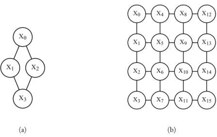
Figure 2.2 shows two Markov networks structures, (a) is an example of a Markov network that encodes conditional independence constraints that can not be perfectly modeled using a Bayesian network (any Bayesian network will have either less or more conditional independence assertions); (b) is an example of a grid structure that is widely used in many computer vision and image processing applications Wang et al. (2013).

(28)

Burglary Alarm JohnCalls MaryCalls Earthquake (a) Season Sprinkler Rain WetGrass Slippery (b)

Figure 2.1 – Examples of Bayesian networks Pearl (1995); Koller and Friedman (2009). Each node is associated with a random variable and a conditional probability distribu-tion. (a) is the burglar alarm Bayesian network. (b) is known as the sprinkler network.

2.1.1 Inference in Probabilistic Graphical Models

Inference in PGMs is the task of answering probabilistic queries, such as the marginal prob-ability of some variablesY, i.e.Pr(Y), or the conditional probability of some variablesYgiven the values of other variablesE, i.e.,Pr(Y|E), whereEis usually called the evidence. Both exact and approximate inference are known to be computationally hard, where the former is #P-Hard and the later is NP-hard Valiant (1979); Dagum and Luby (1993).

Exact inference in PGMs can be done using the variable elimination algorithm. Other ex-act inference algorithms, such as junction trees and the Cutset-conditioning algorithm can be seen as variants of the variable elimination algorithm. The next example demonstrates how the algorithm works using a small concrete example.

(29)

2.1. Probabilistic Graphical Models X0 X1 X2 X3 (a) X0 X1 X4 X2 X5 X3 X6 X7 X8 X9 X10 X11 X12 X13 X14 X15 (b)

Figure 2.2 – Examples of two Markov network structures, (a) is an example of a Markov network that encodes conditional independencies that can not be perfectly modeled us-ing a Bayesian network (any Bayesian network will have either less or more conditional independence assertions); (b) is an example of a grid structure that is widely used in many computer vision and image processing applications Wang et al. (2013).

Example 2.1 (Variable Elimination Algorithm)

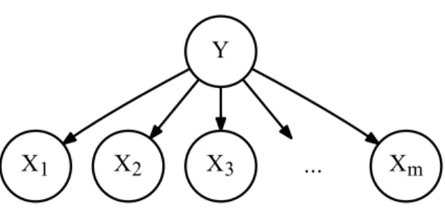
Consider the Bayesian networks in Figure 2.3. The network has m + 1 binary random

variables. Each variable is represented by a node in the graph and edges correspond to depen-dencies between the variables. Assume that we want to compute the marginal probability of

X1 =T rue, i.ePr(X1 = True). One way to compute the marginal is by enumerating the

entire joint distribution and summing the entries that are consistent withX1 =T rue:

Pr(X1 = True) = X Y X X2 X X3 ...X Xm Pr(X1 = True,Y,X2,X3, ...,Xm) | {z } A

(30)

X1 X2 X3 ... Xm

Y

Figure 2.3 – An example Bayesian network withm+ 1variables. Each variable is rep-resented by a node in the graph and edges correspond to dependencies between the variables. This structure is also known as the Naive Bayes model.

a giant table with 2m+1 entries. We can exploit the structure of the Bayesian network to

substitute the termAwith the small factored Conditional Probability Tables (CPTs) that are

associated with the nodes in the Bayesian network:

Pr(X1 = True) = X Y X X2 X X3 ...X Xm

Pr(Y)Pr(X1 = True|Y)Pr(X2|Y)Pr(X3|Y)...Pr(Xm|Y)

=X Y X X2 X X3 ...X Xm

f0(Y)f1(X1 = True,Y)f2(X2,Y)f3(X3,Y)...fm(Xm,Y)

In the second step we used the notationfi(X), whereXcan be a set of variables, to denote a

tabular representation of the CPTs;fi(X)is called a factor andXis its scope. To eﬃciently

compute the previous equation we can utilize the dynamic programming technique by pushing the sums inside the product and store the intermediate results in new temporary factors.

(31)

2.1. Probabilistic Graphical Models Pr(X1 = True) = X Y f0(Y)f1(X1 = True,Y) X X2 f2(X2,Y) X X3 f3(X3,Y)... X Xm fm(Xm,Y) | {z } fm+1(Y) | {z } fj(Y) | {z } fk(Y)

Each new intermediate factor is the result of summing out a variable after multiplying all the factors that include the variable in their scopes. The factor multiplication operation is a binary operation that takes two factorsfi(X)andfj(Y)and returns a new factor that has

a scope ofX∪Y.

The order in which the summations are performed is called theelimination order. In the previous example the order was:X_m, X_m₋₁, ..., X₃, X₂, Y.

The elimination order has a large impact on the efficiency of the variable elimination algo-rithm. This is mainly due to two related facts: 1) the factor multiplication operation returns a new factor with a scope that is the union of its operands’ scopes, 2) a tabular representation for factors is exponential in the size of its scope. So, while one elimination order can be very efficient, another one might produce intractable intermediate factors. In the previous example, each elim-ination step other than the last one produces a new intermediate factor with scope{Y}and each multiplication is between two factors, one with the scope{X_i, Y}, i∈ 1, ..., mand the other with the scope{Y}. Hence, the largest produced factor has a scope of size 2.

Now let us look into an example where an inefficient elimination order is used: Example 2.2 (Inefficient Elimination Order)

(32)

we perform variable elimination using the elimination orderY, Xm, Xm−1, ..., X3, X2 we

will get the following:

Pr(X1 = True) = X X2 X X3 ...X Xm X Y

f0(Y)f1(X1 = True,Y)f2(X2,Y)f3(X3,Y)...fm(Xm,Y)

| {z }

fm+1(X1,X2,X3,...,Xm)

The resulting intermediate factorfm+1 has the scope of X1, X2, X3, ..., Xm and requires

O(2m)space for its representation.

For some special structures the optimal elimination order is known. For example, if the struc-ture is a polytree, an optimal elimination order consists of eliminating singly connected nodes first. However, for arbitrary structures, finding the optimal elimination order is an NP-Hard problem.

The variable elimination algorithm is outlined in Algorithm 2.1. It takes as inputs a set of factorsFand an ordered set O of the variables. The algorithm iterates overO and for each

v ∈ Oit constructs a new factor by multiplying all the factors that involvev, summing out the variablev, then remove all the factors that involvevfromF.

Algorithm 2.1: Variable Elimination

Input:F: Set of local probablistic models

O: Elimination order foreachv ∈ Odo relatedF← {f ∈F:v ∈Scope(f)}; otherF←F−relatedF; newf ←P v Q f∈relatedFf; F←otherF∪ {newf}; returnQ f∈Ff

(33)

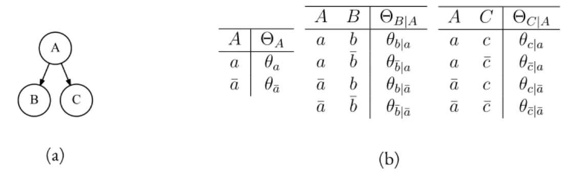
Figure 2.4 – The Bayesian network that is used in Example 2.3, (a) shows the structure of the network, and (b) the conditional probability tables for the variables A, B, and C from left to right.

2.2 Network Polynomials

A network polynomial Darwiche (2000) is a function that encodes a joint distribution such that it can be evaluated in order to answer probabilistic queries. The next example demonstrates this idea by showing a function that encodes the joint distribution of three variables.

Example 2.3 (A Function That Encodes A Joint Distribution)

Consider the Bayesian network in Figure 2.4. The network has three binary random vari-ables. The ﬁgure shows the structure and also shows the conditional probability tables for the three variables. We used the notationxandx¯to denote the true and false values of variable

X, respectively. The joint distribution table is the result of the Cartesian product of the three

(34)

A B C P(A, B, C) a b c θa·θb|a·θc|a a b c¯ θa·θb|a·θ¯c|a a ¯b c θa·θ¯_b|a·θc|a a ¯b c¯ θa·θ¯_b_|_a·θ¯c|a ¯ a b c θ¯a·θb|a¯·θc|¯a ¯ a b c¯ θ¯a·θb|a¯·θ¯c|¯a ¯ a ¯b c θ¯a·θ¯_b_|_a_¯·θc|¯a ¯ a ¯b c¯ θ¯a·θ¯_b_|_a_¯·θ_¯_c|¯a

For each variable we can introduce two indicatorsIxandIx¯, where every indicator can take

either the value of 1 or 0. Using these indicators we can write a function that encodes the joint distribution table as follows:

f =_Ia·Ib ·Ic·θa·θb|a·θc|a +_Ia·Ib ·I¯c·θa·θb|a·θ¯c|a +_Ia·I¯_b ·_Ic·θa·θ¯_b_|_a·θc|a +_Ia·I¯_b ·_I¯c·θa·θ¯_b|a·θ¯c|a +_I¯a·Ib ·Ic·θa¯·θb|¯a·θc|¯a +_I¯a·Ib ·I¯c·θa¯·θb|¯a·θ¯c|¯a +_I¯a·I¯_b ·_Ic·θa¯·θ¯_b_|_¯_a·θc|¯a +_I¯a·I¯_b ·_I¯c·θa¯·θ¯_b_|_¯_a·θ¯c|¯a (2.1)

(35)

2.2. Network Polynomials

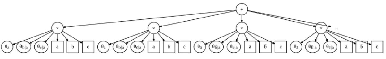
θ_a θ_b|a θ_c|a a b c θ_a θ_b|a θ_c̄|a a b c̄ θ_ā θ_b�|a θ_c|a ā b� c θ_ā θ_b�|a θ_c̄|a ā b� c̄ +

× × × × ...

Figure 2.5 – An arithmetic circuit of the function in Equation 2.1

The previous function was obtained by multiplying each row in the probability table of the joint distribution with the indicators that are consistent with the row. To use the previous function for inference, we can simply replace each indicator with the value of the evidence. For example, if we want to computeP(a, b,c¯)we will set_Ia, Ib, andI¯cto 1 and set all the

other indicators to 0. The result after evaluating the function will beθa·θb|a·θc¯|a, which is the

probability of the assignment according to the Bayesian network. The function in Equation 2.1 can be graphically represented using an arithmetic circuit as shown in Figure 2.5.

A multi-linear function that encodes a joint distribution, similar to the one in Equation. 2.1, is called anetwork polynomialDarwiche (2003). Darwiche shows that many probabilistic queries can be obtained in a time that is linear in the size of the network polynomial by evaluating the network polynomial or evaluating its partial derivatives with respect to the indicators. However, the size of the network polynomial itself will grow exponentially in the number of variables if it was constructed naively as in the previous example. In the same work, Darwiche proposes the use of arithmetic circuits as a graphical representation of the network polynomial. He also proposes the use of the junction tree algorithm as a mean to construct compact arithmetic circuits. This process is known in the literature ascompilation. Although this process can produce arithmetic circuits that are more compact than those obtained by straight forward evaluation, it suffers from two major drawbacks. First, it assumes that the structure and the parameters are known. Second,

(36)

of the junction tree; hence, it is prone to becoming intractable.

A method that focuses on learning arithmetic circuits directly from data was developed in Lowd and Domingos (2012). The method is based on the search-and-score technique, with a score function that prefers compact models by penalizing models that have more edges. The method avoided the need to compile the Bayesian network for each candidate structure by incrementally building the arithmetic circuit.

2.3 Sum-Product Networks

Sum-product networks (SPN) Poon and Domingos (2011) have recently emerged as a new class of tractable probabilistic graphical models. Unlike Bayesian and Markov networks where inference may be exponential in the size of the network as shown above, inference in SPNs is lin-ear in the size of the network. Also, contrary to Bayesian networks and Markov networks where we have separate representations and inference algorithms, SPNs can be seen as both graphi-cal representations and inference machines at the same time. An SPN is defined using a rooted DAG whose internal nodes are either sum or product nodes, and the leaves are indicators of the random variables. Each child of a sum node has an associated weight.

Definition 2.3 (Sum-Product Network Poon and Domingos (2011))

A sum-product network (SPN) overnbinary variablesX1, ..., Xnis a rooted directed

acyclic graph whose leaves are the indicatorsIx1, ..., Ixn and Ix¯1, ..., I¯xn, and whose internal nodes are sums and products. Each edge(i, j)emanating from a sum node

i has a non-negative weight,wij. The value of a product node is the product of the

values of its children. The value of a sum node isP

(37)

2.3. Sum-Product Networks set of children ofiandvj is the value of nodej. The value of an SPN is the value of

its root.

Thescopeof a node is the set of variables that appear in the sub-SPN rooted at that node. The scope of a leaf node is the variable that the indicator refers to and the scope of an interior node is the union of the scopes of its children.

The value of an SPN could be seen as the output of a network polynomial whose variables are the indicator variables and the coefficients are the weights Darwiche (2003). This polyno-mial represents a joint probability distribution over the variables involved if the SPN satisfies the following two properties Poon and Domingos (2011):

Definition 2.4 (Completeness Poon and Domingos (2011))

An SPN is complete iff all children of the same sum node have the same scope, where the scope is the set of variables that are included in a child.

Definition 2.5 (Decomposability Poon and Domingos (2011))

An SPN is decomposable iff no variable appears in more than one child of a product node.

An SPN that is both complete and decomposable isvalid, and it correctly computes a joint distribution over the variables in its scope. The next example shows several basic distributions represented as SPNs.

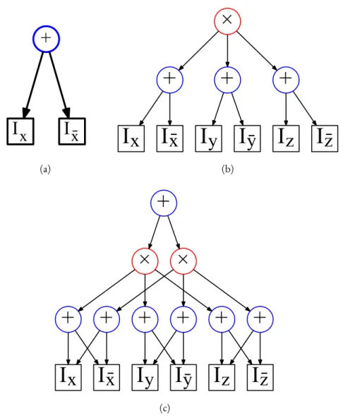
Example 2.4 (Basic distributions encoded as SPNs)

Several basic distributions are encoded by SPNs exhibiting simple structures. For instance, a univariate distribution can be encoded using an SPN whose root node is a sum that is linked to each indicator of a single variableX(see Fig. 2.6(a)). A factored distribution over a set of

(38)

variablesX1, ..., Xnis encoded by a root product node linked to univariate distributions for

each variableXi(see Fig. 2.6(b)). A naive Bayes model is encoded by a root sum node linked

to a set of factored distributions (see Fig. 2.6(c)).

2.3.1 Inference in Sum-Product Networks

Inference about the joint probability of the variables in the scope of an SPNs can be answered by replacing the indicators with either 0 or 1 then perform a bottom up pass. If the value of a variableX = True, then we set the corresponding indicator_I_x = 1and the other indicator

I¯x = 0. IfX = False, then we setIx = 0andIx¯ = 1. If we want to marginalize out a variable

X, then we set_I_x = 1and_I_x_¯ = 1. Conditional inference queriesPr(X = x|Y = y)can be answered by taking the ratio of the values obtained by two bottom up passes of an SPN. In the first pass, we initialize_I_x = 1,_I_x_¯ = 0,_I_y = 1,_I_y_¯ = 0and set all remaining indicators to 1 in order to compute a value proportional to the desired query. In the second pass, we initialize_I_y =

1,_I_y_¯ = 0and set all remaining indicators to 1 in order to compute the normalization constant. The linear complexity of inference in SPNs is an appealing property given that inference for other models such as Bayesian networks is exponential in the size of the network in the worst case.

2.3.2 Learning Sum-Product Networks

Poon and Domingo Poon and Domingos (2011) propose two algorithms to directly learn the parameters of SPNs from data: maximization and gradient descent. The expectation-maximization algorithm relies on interpreting the sum nodes as latent random variables. The gradient descent algorithm uses the partial derivatives of the network polynomial encoded by

(39)

2.3. Sum-Product Networks the SPN. These partial derivatives can easily be obtained by performing a bottom-up pass fol-lowed by a top-down pass, where in the first pass we perform inference as described in the pre-vious subsection and in the second pass we apply the chain rule of derivatives. A discriminative parameter learning algorithm has been proposed in Gens and Domingos (2012) and a Bayesian learning algorithm has also been recently proposed in A. Rashwan (2016). A discussion about these two algorithms is presented in Section 4.2. Several algorithms have been proposed to learn the structure of SPNs Rooshenas and Lowd (2014); Gens and Domingos (2013). In Section 5.4.1 we develop a structure learning algorithm that generalizesLearnSPN()to decision problems.

LearnSPN()is a recursive top-down structure learning algorithm for SPNs. Given a dataset,

LearnSPN()tries first to partition the random variables into independent subsets using an in-dependence statistical test, such asχ2 or G-test. If such a partitioning is found, the algorithm introduces a product node, where each child of the product node correspond to one of the found subsets. If no independent subsets are found, the algorithm introduces a sum node and clusters the dataset into similar instances; each cluster will be associated with one of the sum node’s chil-dren. The algorithm recursively repeats these steps until only one variable is left in the dataset, at which point it introduces a univariate distribution over that variable.

(40)

I

_x

I

_x̄

+

(a)

I

_x

I

_x̄

+

I

_y

I

_ȳ

+

I

_z

I

_z̄

+

×

(b)

I

_x

I

_x̄

I

_y

I

_ȳ

I

_z

I

_z̄

+

×

+

×

+

(c)

Figure 2.6 – Basic distributions encoded as SPNs. (a) shows an SPN that encodes a univariate distribution over a binary variablex. (b) shows an SPN that encodes factored distribution over three binary variablesx,y, andz. (c) is an SPN that encodes a naive Bayes model over three binary variablesx,y, andz. The root sum node corresponds to a the hidden class variable.

(41)

Chapter

3 Dynamic Sum-Product Networks

3.1 Introduction

This chapter presents Dynamic Sum-Product Networks (DynamicSPNs), an extension to SPNs that model sequence data of varying length. The time for inference in DynamicSPNs is guaranteed to always be linear in the size of the network even if some or all the random variables were not observed. Similar to Dynamic Bayesian networks (DBNs) Dean and Kanazawa (1989); Murphy (2002),DynamicSPNs consist of atemplate networkthat repeats as many times as the length of a data sequence. I describe an invariance property for the template network that is suf-ficient to ensure that the resultingDynamicSPNis valid (i.e., encodes a joint distribution) by being complete and decomposable. Since existing structure learning algoritms for SPNs assume a fixed set of variables and fixed-length data, they cannot be used to learn the structure of a Dy-namicSPN. This chapter presents a general anytime search-and-score framework with a specific local search technique to learn the structure of the template network that defines aDynamicSPN based on data sequences of varying length. I demonstrate the advantages ofDynamicSPNs over

(42)

static SPNs, DBNs, and HMMs with synthetic and real sequence data.

3.2 Related Models

3.2.1 Dynamic Arithmetic Circuits

An extension to network polynomials for DBNs was given in Brandherm and Jameson (2004). The proposed procedure compiles a DBN into a recursive network polynomial, where each net-work polynomial for time stept is a function of the network polynomial of time stept −1. The output of each time step’s network polynomial is a table over the Cartesian product of the values of the variables in the belief state (the nodes at time stept−1that are parents of nodes at time stept). The recursive network polynomial can, essentially, be obtained by performing variable elimination with a specified order on the DBN. The recursive network polynomial can be represented with a special AC that has multiple roots and placeholders to plug the roots of the previous time step’s network polynomial. I call this representation Dynamic Arithmetic Cir-cuits (Dynamic ACs). Dynamic ACs are compiled representations, which means that we have to start from a known DBN and then convert it to a Dynamic AC. There is a risk that the compiled Dynamic AC will be intractable because of the the size of the output table or the internal repre-sentation. For the output table, the authors proposed to use the Boyen-Koller Boyen and Koller (1998) method to approximate the large output table with several smaller ones. The internal rep-resentation, on the other hand, may still suffer of an exponential blow up since it depends on the variable elimination order and have the same complexity as the variable elimination algorithm. Thus, compiling a DBN to a Dynamic AC does not reduce the complexity of inference, but only makes it linear in the size of the compiled Dynamic AC, which could be intractable. In this

(43)

3.2. Related Models work I present a model that can be learned directly from data and present a structure learning algorithm that guarantees to find tractable models.

3.2.2 Dynamic Bayesian Networks

As we have seen in Section 2.1, Bayesian networks are defined over a fixed number of vari-ables. Dynamic Bayesian Networks (DBNs) extend Bayesian networks to the dynamic setting by defining a template structure that can be instantiated for sequences of varying lengths Mur-phy (2002); Koller and Friedman (2009). A DBN is defined as a pairhB₁,B_→i, whereB₁is a Bayesian network that defines the initial distribution, andB_→is a two-time-slice Bayesian net-work (2TBN) that defines the conditional distribution of the random variables at time stept given the variables at time stept −1. Parameters learning in DBNs can be done by tying the parameters across time slices. REVEAL Liang et al. (1998) is a greedy search-and-score structure learning algorithm for DBNs that focuses on capturing the dynamics of the variables between the time steps. Given a data instance of lengthT, inference can be done byunrollingthe DBN forT time slices. The unrolled version is a regular Bayesian networks; hence, we can use any of the inference algorithms for Bayesian networks. The problem with this approach is of two folds. First,T can be arbitrarily large, which would make the unrolled Bayesian network large as well. Second, common inference tasks in DBNs require maintaining abelief stateover time, which is a distribution over the variables at time steptgiven all the previous observations. The exact representation of the belief state is exponentially large in the number of hidden variables. Some inference algorithms, such as Boyen-Koller Boyen and Koller (1998) and the factored frontier algorithm Murphy and Weiss (2001), tackle this problem by approximating the belief state using a product of marginals of some cluster of variables.

(44)

3.3 Dynamic Sum-Product Networks

Sequence data such as time series data is typically generated by a dynamic process. Such data is conveniently modeled using structure that may be repeated as many times as the length of the process and a way to model the dependencies between the repeated structure. In this context, we propose dynamic SPNs (DynamicSPNs) as a generalization of SPNs for modeling sequence data of varying length. This is motivated by the fact that if aDynamicSPNis a valid SPN, then inference queries can be answered in linear time thereby providing a way to perform tractable inference on sequence data.

As an example, consider temporal sequence data that is generated bynvariables (or features) overT time steps:

D

hX1, X2, . . . , Xni1,hX1, X2, . . . , Xni2, . . . ,hX1, X2, . . . , XniT

E

whereX_i,i= 1. . . nis a random variable in one time slice andT may vary with each sequence. Note that non-temporal sequence data such as sentences (sequence of words) can also be repre-sented by sequences of repeated features. We will label the set of repeating variables as asliceand we will index slices byteven if the sequence is not temporal, for uniformity.

ADynamicSPNmodels sequences of varying length with a fixed number of parameters by using a template that is repeated at each slice. This is analogous to DBNs where the template corresponds to the network that connects two consecutive slices. We define the template SPN for each slicehX₁, X₂, . . . , X_niT as follows.

(45)

3.3. Dynamic Sum-Product Networks

Definition 3.1 (Template network)

A template network for a slice ofnbinary variables at timet,hX1, X2, . . . , Xnit, is

a directed acyclic graph withkroots andk+ 2nleaf nodes. The2nleaf nodes are the

indicator variables,I_xt

1, Ixt2, . . . , Ixtn, Ix¯1t, Ix¯t2, . . . , Ix¯tn. The remainingkleaves and an equal number of roots are interface nodes to and from the template for the previous and next slices, respectively. The interface and interior nodes are either sum or product nodes. Each edge(i, j)emanating from a sum node ihas a non-negative weight wij

as in a SPN. Furthermore, we deﬁne a bijective mappingf between the input and

output interface nodes.

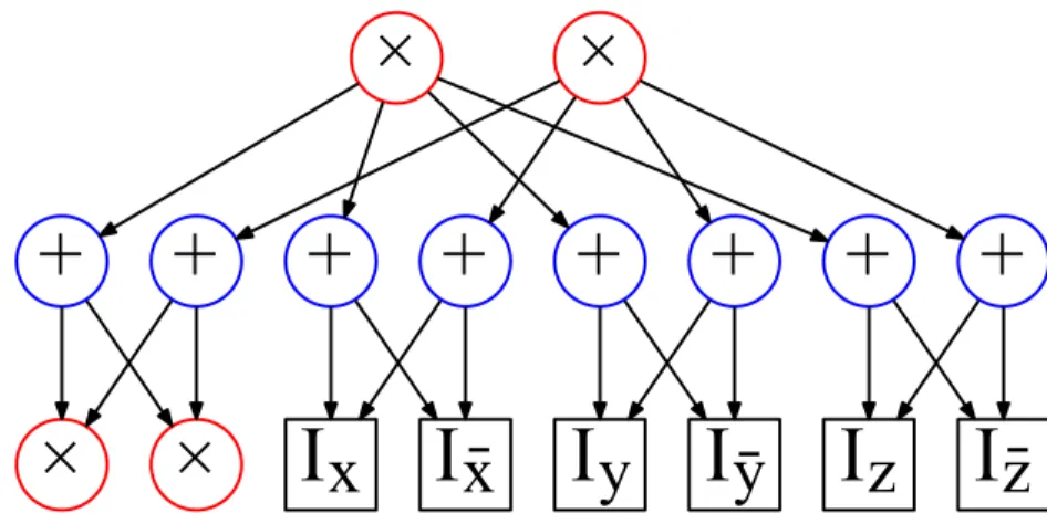
A generic template network is shown in Fig. 3.1.

I

_x

I

_x̄

I

_y

I

_ȳ

I

_z

I

_z̄

×

+

×

+

×

Figure 3.1 – An example of a generic template network. Notice the interface nodes in red.

(46)

Definition 3.2 (Bottom network)

A bottom network for the ﬁrst slice of n binary variables,hX1, X2, . . . , Xni1, is a

directed acyclic graph with k roots and 2n leaf nodes. The 2n leaf nodes are the

indicator variables,I_x1

1, Ix12, . . . , Ix1n, I¯x11, Ix¯12, ..., I¯x1n. Thekroots are interface nodes to the template network for the next slice. The interface and interior nodes are either sum or product nodes. Each edge (i, j) emanating from a sum node i has a

non-negative weightwij as in a SPN.

Definition 3.3 (Top network)

Deﬁne a top network as a rooted directed acyclic graph composed of sum and product nodes withk leaves. The leaves of this network are interface nodes, which were

intro-duced previously. Each edge(i, j)emanating from a sum nodeihas a non-negative

weightwij as in a SPN.

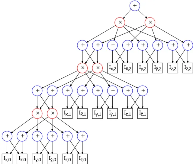
ADynamicSPNis obtained by stacking as many copies of the template network of Def. 3.1 as the number of slices in a sequence less 1 on top of a bottom network. This is capped by a top network. Two copies of the template are stacked by merging the input interface nodes of the up-per copy with the output interface nodes of the lower copy. A template is stacked on a bottom network by merging the output interface nodes of the bottom network with the input inter-face nodes of the template. Analogously, the top network is stacked on a template by merging the input interface nodes of the top network with the output interface nodes of the template. Figure 3.2 shows an example with 3 slices of 2 variables each.

While aDynamicSPNconforms to the structure required of a SPN, we note that the bot-tom, template and top networks are not SPNs when considered separately. The bottom and

(47)

3.3. Dynamic Sum-Product Networks I_x,0 I_x,0 I_y,0 I_ȳ_,0 I_z,0 I_z,0 + + + × + + + × + + I_x,1 I_x,1 I_y,1 I_ȳ_,1 I_z,1 I_z,1 + + + × + + + × + + I_x,2 I_x,2 I_y,2 I_ȳ_,2 I_z,2 I_z,2 + + + × + + + × +

Figure 3.2 – A generic example of a completeDynamicSPNunrolled over 3 time slices. Template network is stacked on the bottom network and capped by the top network. template networks have multiple roots while an SPN has a single root. The template and top networks also have leaves that are not indicator variables while all the leaves of an SPN are indi-cator variables.

As we mentioned previously, completeness and decomposability are sufficient to ensure the validity of an SPN. While one could check that each sum node in theDynamicSPNis complete

(48)

and each product node is decomposable, we provide a simpler way to ensure that any Dynam-icSPNis complete and decomposable. In particular, we describe an invariance property for the template network that can be verified directly in the template without unrolling the Dynamic-SPN. This invariance property is sufficient to ensure that completeness and decomposability are satisfied in theDynamicSPNfor any number of slices.

Definition 3.4 (Invariance)

A template network over hX1, ..., Xnit is invariant when the scope of each input

interface node excludes variables {Xt

1, ..., Xnt} and for all pairs of input interface

nodes,iandj, the following properties hold:

• scope(i) =scope(j)∨scope(i)∩scope(j) = ∅

• scope(i) =scope(j) ⇐⇒ scope(f(i)) =scope(f(j))

• scope(i)∩scope(j) =∅ ⇐⇒ scope(f(i))∩scope(f(j))=∅

• all interior and output sum nodes are complete

• all interior and output product nodes are decomposable

Here f is the bijective mapping that indicates which input nodes correspond to

which output nodes in the interface.

Intuitively, a template network is invariant if we can assign a scope to each input interface node such that each pair of input interface nodes have the same scope or disjoint scopes, and the same relation holds between the scopes of the corresponding output nodes. Scopes of pairs of corre-sponding interface nodes must be the same or disjoint because a product node is decomposable

(49)

3.3. Dynamic Sum-Product Networks when its children have disjoint scopes and a sum node is complete when its children have iden-tical scope. Hence, verifying the identity or disjoint relation of the scopes for every pair of input interface nodes helps us in verifying the completeness and decomposability of the remaining nodes in the template. Note that the invariance property is only concerned with the validity of the resulting unrolled SPNs and it does not imply that the process is stationarity. Theorem 3.1 below shows that the invariance property of Def. .1 can be used to ensure that the corresponding DynamicSPNis complete and decomposable.

Theorem 3.1

If (a) the bottom network is complete and decomposable, (b) the scopes of all pairs of output interface nodes of the bottom network are either identical or disjoint, (c) the scopes of the output interface nodes of the bottom network can be used to assign scopes to the input interface nodes of the template and top networks in such a way that the template network is invariant and the top network is complete and decomposable, then the correspondingDynamicSPNis complete and decomposable.

Proof. Below, I sketch a proof by induction (see Appendix A for more details). For the base case, consider a single-sliceDynamicSPNthat contains the bottom and top networks only. The bot-tom network is complete and decomposable by assumption. Since the interface output nodes of the bottom network are merged with the input interface nodes of the top network, they are assigned the same scope, which ensures that the top network is also complete and decompos-able. Hence a single-sliceDynamicSPNis complete and decomposable. For the induction step, assume that aDynamicSPNofT slices is complete and decomposable. Consider a Dynamic-SPNofT + 1slices that shares the same bottom network and the same firstT −1copies of

(50)

T −1copies of the template network in theDynamicSPNofT + 1slices are complete and decomposable. Since the next copy of the template network is invariant when its input interface nodes are assigned the scopes with the same identity and disjoint relations as the scopes of the output interface nodes of the bottom network, it is also complete and decomposable. Similarly the top network is complete and decomposable since its interface nodes inherit the scopes of the interface nodes of the template network which have the same identity and disjoint relations as the output interface nodes of the bottom network. HenceDynamicSPNs of any length are complete and decomposable.

In summary, aDynamicSPNis an SPN with a repeated structure and tied parameters spec-ified by the template. The likelihood of a data sequence can be computed by instantiating the indicator variables accordingly and propagating the values to the root. Hence inference can be performed in linear time with respect to the size of the network.

3.4 Structure Learning of DynamicSPNs

As aDynamicSPNis an SPN, we could ignore the repeated structure and learn an SPN for the number of variables corresponding to the longest sequence. Shorter sequences could be treated as sequences with missing data for the unobserved slices. Unfortunately, this is in-tractable for very long sequences because the inability to model the repeated structure implies that the SPN will be very large and the learning computationally intensive. This approach may be feasible for datasets that contain only short sequences, nevertheless the amount of data needed may be prohibitively large because in the absence of a repeating structure the number of param-eters is much higher. Furthermore, the SPN could be asked to perform inference on a sequence

(51)

3.4. Structure Learning of DynamicSPNs Alternately, it is tempting to apply existing algorithms to learn the repeated structure of the DynamicSPN. Unfortunately, this is not possible. As existing algorithms assume a fixed set of variables, one could break data sequences into fixed-length segments corresponding to each slice. An SPN can be learned from this dataset of segments. However, it is not clear how to use the resulting SPN to construct a template network because a regular SPN has a single root while the template network has multiple roots and an equal number of input leaves that are not indicator variables. One would have to treat each segment as independent data instances and could not answer queries about the probability of some variables in one slice given the values of other variables in other slices.

This section presents ananytime search-and-scoreframework to learn the structure of the template SPN in aDynamicSPN. Algorithm 3.1 outlines the local search technique that itera-tively refines the structure of the template SPN. It starts with an arbitrary structure and then generates several neighbouring structures. It ranks the neighbouring structures according to a scoring function and selects the best neighbour. These steps are repeated until a stopping crite-rion is met. This framework can be instantiated in multiple ways based on the choice for the ini-tial structure, the neighbour-generation process, the scoring function and the stopping criterion. We proceed with the description of a specific instantiation below, although other instantiations are possible.

Without loss of generality, we propose to use product nodes as the interface nodes for both the input and output of the template network.1 I also propose to use a bottom network that is identical to the template network after removing the nodes that do not have any indicator

1

WLOG assume that theDynamicSPNalternates between layers of sum and product nodes. Since a

Dynam-icSPNconsists of a repeated structure, there is flexibility in choosing the interfaces of the template. I chose the interfaces to be at layers of product nodes, but the interfaces could be shifted by one level to layers of sum nodes or even traverse several layers to obtain a mixture of product and sum nodes. These boundaries are all equivalent

(52)

Algorithm 3.1: LearnDynamicSPN(): Anytime Search-and-Score Framework for Dy-namicSPNs

Input: data,

hX1, ..., Xni: set of variables for a slice

Output:templN et: template network

templN et←initialStructure(data,hX1, ..., Xni); repeat

templN et←neighbour(templN et, data); untilstopping criterion is met;

variable as descendent. This way we can design a single algorithm to learn the structure of the template network since the bottom network will be automatically determined from the learned template. I also propose to fix the top network to a root sum node directly linked to all the input product nodes. For the template network, we initialize the SPN rooted at each output product node to a factored model of univariate distributions. Figure 3.1 shows an example of this ini-tial structure with two interface nodes and three variables. Each output product node has four children where each child is a sum node corresponding to a univariate distribution. Three of those children are univariate distributions linked to the indicators of the three variables, while the fourth sum node is a distribution over the interface input nodes. On merging the interface nodes for repeated instantiations of the template, we obtain a hierarchical mixture model. We begin with a single interface node and iteratively increase their number until the score produced by the scoring function stops improving. Algorithm 3.2 summarizes the steps to compute the initial structure. It is worth noting that any template network that satisfies the invariant prop-erty can be used as an initial structure. Hence, one can easily develop a version of the structure learning algorithm with random restarts by having different initial structures and wrapping Al-gorithm 3.1 inside a loop for the restarts.

Directly Learning Tractable Models for Sequential Inference and DecisionMaking