1
Accuracy, Scalability, and Efficiency of Mixed-Element
USM3D for Benchmark Three-Dimensional Flows
Mohagna J. Pandya1
NASA Langley Research Center, Hampton, Virginia 23681, USA
Dennis C. Jespersen2
NASA Ames Research Center, Moffett Field, California 94035, USA
Boris Diskin3
National Institute of Aerospace, Hampton, Virginia 23666, USA and
James L. Thomas4, Neal T. Frink5
NASA Langley Research Center, Hampton, Virginia 23681, USA
The unstructured, mixed-element, cell-centered, finite-volume flow solver USM3D is enhanced with new capabilities including parallelization, line generation for general unstructured grids, improved discretization scheme, and optimized iterative solver. The paper reports on the new developments to the flow solver and assesses the accuracy, scalability, and efficiency. The USM3D assessments are conducted using a baseline method and the recent hierarchical adaptive nonlinear iteration method framework. Two benchmark turbulent flows, namely, a subsonic separated flow around a three-dimensional hemisphere-cylinder configuration and a transonic flow around the ONERA M6 wing are considered.
I. Introduction
Government agencies and industry rely heavily on computational aerodynamic analysis and design tools for conducting fundamental and applied aerodynamic research, and for cost-effective modification/development of air vehicles. Computational Fluid Dynamic (CFD) methods have led to a more strategic utilization of wind-tunnel and flight-test resources. CFD methods play an important role for the attached-flow design conditions. However, it is broadly recognized that large solution uncertainties exist in CFD solutions for the massively-separated turbulent flows encountered at off-design conditions. A recent NASA-sponsored CFD Vision 2030 study recognizes this limitation and provides several recommendations for the development of a comprehensive roadmap to address CFD grand challenge problems [1].
The NASA Revolutionary Computational Aerosciences (RCA) subproject under the Transformational Tools and Technologies project is engaged in foundational research focused on identifying and down-selecting critical turbulence, transition, and numerical method technologies for challenging turbulent separated flows, evolution of free shear flows, and shock-boundary layer interactions. The separated flow regime has proved to be challenging for the traditional turbulence models based on the Reynolds Averaged Navier-Stokes (RANS) approach. The quest for increased accuracy for massively-separated flows has evoked interest in alternative paradigms such as Large Eddy Simulation (LES) and hybrid RANS-LES approaches. These alternative approaches require long duration time-accurate simulations on higher resolution grids and thereby demand tremendous computational resources. The accurate approaches need to be accompanied by new robust and efficient solution methodologies such that a
1Research Aerospace Engineer, Configuration Aerodynamics Branch, Mail Stop 499, Senior Member AIAA. 2Computer Scientist, Advanced Computing Branch, NASA Advanced Supercomputing Division, Mail Stop 258-5. 3NIA Research Fellow, Associate Fellow AIAA.
4Distinguished Research Associate, Computational Aerosciences Branch, Mail Stop 399, Fellow AIAA. 5Senior Aerospace Engineer, Configuration Aerodynamics Branch, Mail Stop 499, Associate Fellow AIAA.
2
substantial reduction in the time-to-solution can be achieved for routine and increasingly-multidisciplinary analysis and design simulations. The algorithms of the new solution methodologies should be able to adapt to and exploit emerging computer architectures.
Toward this end, a sustained multiyear effort is underway to advance our knowledge and understanding of how to improve the accuracy and efficiency of unstructured cell-centered RANS solver methodology. These advancements are being investigated in a prominent NASA cell-centered Navier-Stokes flow solver, USM3D, which is a part of the NASA Tetrahedral Unstructured Software System (TetrUSS) [2]. This tool set has endured the multiyear rigor of extensive configuration aerodynamic research within NASA [2]-[4], and for product development within major airframe companies [5]-[7]. An overriding attribute of the USM3D flow solver has been its speed and robustness in providing solutions for a broad class of vehicles, which makes it a good candidate for further upgrades.
The current focus is to address RCA’s three pillars of research, namely, accuracy, efficiency, and robustness, keeping in mind the critical role of automation in the CFD solution process. Time reduction of at least two orders of magnitude achieved through algorithmic advancements is the goal for USM3D simulation of complex flows around complex geometries. Encouraging initial strides have been made in this direction already. USM3D has been extended to support the solutions on mixed-element grids [8] that provide improved numerical simulation using flow-aligned anisotropic hexahedral or prismatic cells in a boundary layer and isotropic tetrahedral cells away from a boundary layer. A new solution methodology named as Hierarchical Adaptive Nonlinear Iteration Method (HANIM) [9] has been implemented in the mixed-element USM3D. HANIM is a strong nonlinear solver that improves the robustness, efficiency, and automation of the RANS solutions. HANIM provides two additional hierarchies around a simple preconditioner of USM3D, which is based on a linearization of a simplified discrete formulation and a point-implicit Gauss-Seidel (G-S) relaxation scheme. The HANIM hierarchies are a matrix-free linear solver for the exact linearization of RANS equations and a nonlinear control of the solution update. The goal of these hierarchies is to enhance the iterative scheme with a mechanism for an automatic adaption of the operational pseudotime step to increase convergence rates and overcome transitional instabilities and limit cycles. The matrix-free linear solver [10]-[14] uses the Fréchet derivatives and a Generalized Conjugate Residual (GCR) method [11]. The nonlinear update methodology is close to the one discussed in [14]. The USM3D HANIM methodology using a point-implicit preconditioner was assessed [9] on four turbulent flow benchmark cases, namely, a two-dimensional (2D) zero pressure gradient flat plate, a 2D bump-in-channel configuration, the 2D NACA0012 airfoil, and a three-dimensional (3D) NASA Common Research Model configuration. In that study, the Spalart-Allmaras (SA) eddy viscosity turbulence model [15], [16] was used. The convergence acceleration factor ranging from 1.4 to 13 was demonstrated relative to the USM3D’s baseline preconditioner-alone (PA) solver.
A further enhancement to the efficiency of mixed-element USM3D HANIM was achieved by implementing a line-implicit preconditioner [17]. The line generator used in that study was limited to only prismatic and/or hexahedral cells and imposed restriction that cells must be of the same topology within a given line. Line-implicit iterations simultaneously update a preconditioner solution at all cells of a grid line. An assessment of the iterative convergence of point- and line-implicit preconditioners within the HANIM framework was conducted [17] on two benchmark 3D configurations. The configurations were a bump in a channel and a hemisphere cylinder (H-C). For each configuration, a family of consistently refined grids was used. The study demonstrated that only line-implicit HANIM met convergence targets on all grids. An assessment of time to solution normalized by degrees of freedom showed that the case-to-case variation in the performance of the line-implicit HANIM is significantly less than the corresponding variation in the performance of the point-implicit HANIM. The performance of the line-implicit HANIM is also less sensitive to an increase in degrees of freedom.
The aforementioned studies were performed using a sequential version of the mixed-element USM3D. The current effort is focused on the efficient parallelization of the flow solver. Several additional enhancements in the discretization and linear solver are made to improve the accuracy and efficiency of USM3D. In this paper, the accuracy, scalability, and efficiency of the parallel mixed-element USM3D are assessed on two benchmark 3D configurations, namely, an H-C configuration and the ONERA M6 (OM6) wing. Grids as large as 629 million cells are used for the present assessments. The choice of these two configurations is motivated by the following two factors: (1) Grid generation and coarsening programs [18] that can generate families of uniformly-refined grids and provide adequate and easy control over the grid size, topology of grid elements, and distribution of grid nodes are available, (2) USM3D results can be compared with the results of several other CFD solvers on the same configurations using identical grids available at the NASA Turbulence Modeling Resource (TMR) website [19], [20].
The current paper provides the following new contributions: (1) development and assessment of parallel mixed-element USM3D are described in detail, including parallelization strategy for line-implicit iterations, modifications for nodal averaging scheme, and both scalability and verification studies; (2) a line-generation algorithm suitable for general unstructured grids is presented and assessed; (3) assessment of solution accuracy through grid refinement
3
studies that include the effects of second-order accuracy of the SA model advection; and (4) a detailed solver efficiency study is presented, including assessments of the effects of a grid topology, grid resolution, and convergence criteria.
The material in this paper is organized in the following order. Section II overviews the principal elements of the preceding versions of mixed-element USM3D [8], [9], [17], including HANIM. Section III provides a detailed description of the newly implemented features of USM3D. The computational results are reported in Section IV. Concluding remarks are presented in Section V.
II. Review of the Preceding Mixed-Element USM3D
The salient features of the preceding versions of mixed-element USM3D [8], [9], [17] are described here. USM3D solves a system of nonlinear flow equations that can be formally represented as
𝑹(𝑸) = 0. (1)
The discrete nonlinear operator, 𝑹(𝑸), represents a cell-centered discretization of the steady-state RANS equations. The term “cell-centered” means that the independent variables used by the governing equations are the flow variables defined at the centroid of each cell. The solution variables at the grid nodes and boundary faces as well as the cell and face gradients are computed solely from the current solution variables defined at the cell centers.
A reconstruction process based on solution gradients computed within cells accomplishes the USM3D second-order spatial discretization of inviscid fluxes. The cell gradients for inviscid fluxes are computed by a Green-Gauss integration procedure that uses a nodal solution. Inviscid fluxes are computed at each cell face using various upwind schemes, such as Roe’s Flux Difference Splitting (FDS) [21], van Leer’s Flux Vector Splitting (FVS) [22], Harten, Lax, van Leer, Einfeldt (HLLE) [23], or Harten, Lax, van Leer – Contact (HLLC) [24] schemes, among others. The standard [15] and negative variants [16] of the SA one-equation turbulence model are available. The convective term of the SA turbulence-model equation can be approximated with either second- or first-order accuracy. Face gradients are needed for the diffusion fluxes of the meanflow and turbulence-model equations. A face gradient is evaluated from Mitchell’s stencil [25], [26]. A face-area weighted average of the face velocity gradients provides the cell-based gradients for the SA source term.
The cell-centered solution values are required to satisfy realizability constraints, such as positive density and pressure. For second-order spatial accuracy, a realizability check is implemented for the reconstructed solution to avoid a catastrophic failure (an underflow condition associated with a square root of a negative number) in computing meanflow inviscid fluxes. If a realizability violation is detected at a face during any nonlinear iteration, the face is temporarily designated as “first-order”. The “first-order” designation for a face is removed after the second-order reconstruction values have been realizable for 20 consecutive nonlinear iterations.
A preconditioner is the central component of USM3D’s nonlinear iteration strategies. The USM3D preconditioner computes a solution correction, ∆𝑸, using a defect correction scheme
𝑉 ∆𝜏∆𝑸 + 𝜕𝑹 𝜕𝑸 0 ∆𝑸 = −𝑹(𝑸2), (2) 𝑸245 = 𝑸2+ ∆𝑸. (3)
Here, 𝑸2 and 𝑸245 are the solutions at iterations 𝑛 and 𝑛 + 1, respectively. The term 𝝏𝑹 𝝏𝑸
9 approximates the Jacobian𝝏𝑹 𝝏𝑸,
𝑉 is a control volume and ∆𝜏 is a pseudotime step, which is set through a Courant-Friedrichs-Lewy (CFL) number specification. The meanflow and turbulence-model preconditioner equations are loosely coupled. The approximate Jacobian for the meanflow equations is formed using the linearization of the first-order FVS or FDS inviscid fluxes and a thin-layer approximation for the viscous fluxes. The approximate Jacobian for a turbulence-model equation includes the contributions from the advection, diffusion, and source terms. The advection term is linearized with a first-order approximation. A thin-layer approximation is used for the diffusion term. The entire contribution from the linearized source term is added to the diagonal. A positivity check for the diagonal values is conducted before adding the pseudotime term. Negative diagonal values are substituted by their absolute values. An option to use single precision for the approximate Jacobian off-diagonal terms and for the solution updates is available to reduce the memory footprint.
The preconditioner equation (Eq. (2)) is solved using either point- or line-implicit Gauss-Seidel (G-S) iterations. For the prismatic and hexahedral grids, cell-based grid lines can be generated within USM3D using a simple line generation algorithm. For general unstructured grids, lines need to be generated externally and provided as input. For the line-implicit G-S iterations, a multicolor order is followed. Cells that belong to a specific line are assigned the same color. Cells within neighboring lines cannot have the same color. Same-color cells are updated simultaneously. The multicolor order limits the topological distance (to the number of colors) by which a solution perturbation at a cell can affect solutions at other cells within one preconditioner iteration. For example, Jacobi iteration corresponds
4
to the one-color order and limits the propagation of a perturbation to immediate neighbors. A two-color linear iteration scheme can propagate a perturbation to a neighbor’s neighbor. This localization is important to prevent instabilities in the line-implicit iterations. For example, if implicit lines have an unsuitable grid orientation (i.e., long dimensions of anisotropic cells are aligned with line directions) and solution updates are conducted in a lexicographical order (implying the number of colors equals the number of lines), then line-implicit iterations applied to the linearized inviscid-flow equations can become unstable. Point-implicit iterations do not suffer from this type of instability and can update cell solutions in any order.
USM3D offers two iteration methodologies to advance a nonlinear solution. In the baseline methodology, designated as Preconditioner-Alone (PA) solver, the correction computed by the preconditioner is directly applied to update the current nonlinear solution. The preconditioner uses a fixed number of linear iterations. The CFL variation is specified a priori. The CFL is often ramped over several nonlinear iterations to a maximum value of 150 and then kept unchanged. The other solution methodology is HANIM. HANIM prescribes the residual reduction targets for the preconditioner, GCR, and nonlinear solution updates and specifies the maximum number of linear iterations allowed in the preconditioner and the maximum number of search directions allowed in GCR. Unlike in the PA method, the HANIM CFL update strategy is solution-adaptive. HANIM increases CFL if all the HANIM hierarchies have reported success. On the other hand, if preconditioner, GCR, or nonlinear solution update fails, HANIM discards the suggested correction and aggressively reduces CFL. The preceding mixed-element USM3D was not parallelized, therefore, solutions could only be computed by serial computations using a single Central Processing Unit (CPU).
III. New Developments
This section reports on the recent USM3D developments. The developments include an efficient flow solver parallelization and improvements to the discretization, line-generation capability, and iterative solver.
A. Modification to the Nodal Averaging Method
The nodal averaging method of the preceding mixed-element USM3D is modified for amenability with the flow solver parallelization. Solution at a node is computed as the weighted average of the corresponding solutions defined at the centers of the cells that constitute the nodal stencil. A pseudo-Laplacian method is used to compute weights [27]-[30]. The method is equivalent to a least-squares interpolation [31]. The stencil weights depend on the position vectors (coordinates) of the cell centers relative to the node. In the present code, a revised nodal averaging procedure is implemented that is exclusively based on the natural stencil. For a given node, the natural stencil is composed of the cells that share the specific node. At least four distinct stencil points (cells) are needed for the 3D pseudo-Laplacian procedure. A natural stencil may be degenerate, i.e., not suitable to support a least-squares system for a 3D linear fit. For example, a stencil is degenerate if there are fewer than four points (cells) in the stencil or if all stencil points (cell centers) are located on the same linear subspace (e.g., a 2D plane).
The current procedure to compute the weights for a degenerate natural stencil differs from the treatment of a degenerate natural stencil in the previous version of USM3D [17], where the stencil was augmented (expanded) to render it amenable to a 3D pseudo-Laplacian procedure. An augmented stencil includes cells that do not share the node under consideration. While shown to be efficient in a single-CPU serial implementation, an augmented stencil is inefficient for a parallel implementation based on domain decomposition. In an efficient parallel implementation, each processor should be able to interpolate a solution at all nodes within its partition, including the nodes at the partition interfaces. The augmented stencil may become significantly larger than the natural stencil, dramatically increasing interpartition communication and reducing scalability. Instead of expanding a degenerate natural stencil, the current procedure suitably reduces the dimension of the pseudo-Laplacian method for the node with a degenerate natural stencil. This approach is suitable for parallel computations as it does not increase the interpartition communication. See Section III.C for details of USM3D’s parallelization strategy.
USM3D constructs nodal stencils internally in a preprocessing stage. To identify a degenerate stencil, a global threshold parameter, 𝜀, is used that defines the minimum recognizable distance. For example, if the distance between a plane and a point is less than 𝜀, the point is considered as located on the plane. In the current implementation, ε is 90% of the shortest distance from any cell center to a viscous boundary surface in the global grid. Several conditions are checked to identify the largest dimension of the pseudo-Laplacian procedure for which the natural stencil is not degenerate. If all stencil points are within the distance ε from each other, then all stencil weights are set to unity. If there are two stencil points that are at a distance greater than ε from each other, then these two points can define a line. If all other stencil points are located on this line, then the node is projected onto the line, and the 1D pseudo-Laplacian method is used to compute the weights. If there is a third point in the stencil that is located farther than ε
5
on this plane, then the node is projected onto the plane, and the 2D pseudo-Laplacian method is used to compute the weights. If there is a fourth point in the stencil that is located farther than ε from the plane, then the stencil is not degenerate, and the standard 3D pseudo-Laplacian method is used to compute the weights.
USM3D treats the symmetry boundary nodes differently from the rest of the nodes in the nodal averaging procedure. A lower dimensional (maximum dimension is 2) pseudo-Laplacian procedure defines the nodal averaging weights for the symmetry boundary patch nodes. The implementation relies on certain properties of symmetry patches. In 3D, at most, three distinct symmetry patches can intersect. All faces of a symmetry patch must have the same unit normal (the normalized directed area). This property is strictly enforced and checked within USM3D during the preprocessing stage. To ascertain the dimensionality of the pseudo-Laplacian procedure, all nodes are grouped in four types. Type 0 nodes are all the nodes that are not on a symmetry boundary, type 1 nodes are on a single symmetry boundary patch, type 2 nodes are at the intersection of two symmetry boundary patches, and type 3 nodes are at the intersection of three symmetry boundary patches. Correct identification of a boundary node type in the USM3D parallel framework requires additional interpartition communication that is described in Section III.C.
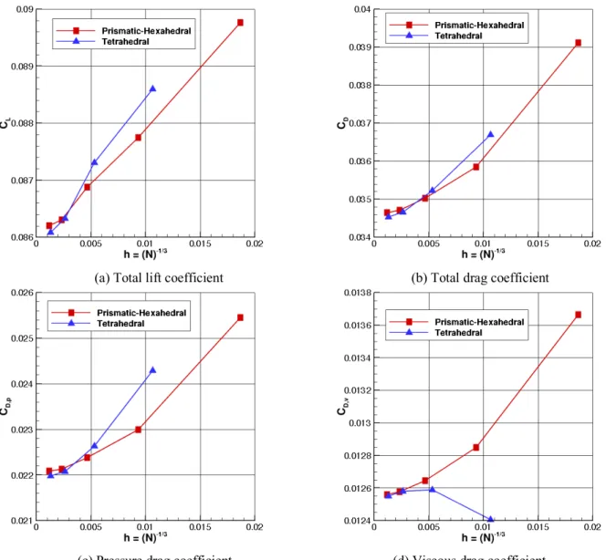
Most of the degenerate-natural-stencil nodes are located on computational boundaries. In the interior of the computational grid, nodes with a degenerate stencil are rare. Tetrahedral elements and boundary curvature lead to a reduction in the number of nodes with a degenerate stencil. This reduction is because with tetrahedral grids, a node has a greater number of stencil points, and boundary curvature often prevents stencil points from being located on a linear subspace. In general, the proportion of the degenerate-stencil nodes relative to the total number of grid nodes is low and decreases on finer grids. To assess the impact of the revised nodal averaging method on nonlinear iterative convergence, three computational cases have been considered: (1) a separated subsonic flow at 19° angle of attack over an H-C configuration, (2) a transonic flow at 3.06° angle of attack over the OM6 wing, and (3) a transonic flow at 2° angle of attack over a NASA Common Research Model (CRM) wing-body-tail configuration that was used for the fourth AIAA Drag Prediction Workshop. The mixed-element grids around the H-C configuration and OM6 wing consist of prismatic and hexahedral cells. The mixed-element grid around the NASA CRM configuration is composed of prismatic, pyramidal, and tetrahedral cells. Table 1 shows the proportion of the degenerate stencil nodes needing various reductions in the dimension of the pseudo-Laplacian procedure, relative to the total number of nodes and cells in the grids.
Table 1 Statistics related to grid density and nodes with degenerate stencil.
Case Grid type Cells Nodes Nodes with
degenerate stencil
Nodes with dimension reduction
1 2 3
H-C Prismatic-Hexahedral 1,228,800 1,143,081 21,925 21,827 98 0
OM6 wing Prismatic-Hexahedral 1,081,344 960,225 6,646 6,646 0 0
NASA CRM Prismatic-Tetrahedral 1,524,325 685,981 2,054 2,046 7 1
For most of the degenerate-stencil nodes, a reduction of just one dimension is sufficient for the application of the pseudo-Laplacian procedure. Nodes that require a greater reduction in the dimensionality are typically located at the intersections of nonsymmetry boundary patches, where the natural stencil has fewer points. The H-C and OM6-wing grids are both composed of prismatic and hexahedral cells. In spite of the fact that the grids have a similar number of nodes, the numbers of nodes with a degenerate stencil differ significantly. This difference is related to the topology of various boundary intersections. The H-C grid has intersections of the outflow-boundary patch with two other nonsymmetry boundary patches, namely, the aerodynamic surface patch and the farfield boundary patch. The OM6-wing grid has no intersections between nonsymmetry boundary patches. The NASA CRM grid is composed of prismatic and tetrahedral cells. The presence of tetrahedral cells substantially reduces the number of nodes with a degenerate stencil. In this grid, there is one node that requires the reduction of three dimensions for the pseudo-Laplacian procedure. This node is one of the farfield-boundary corner nodes that has a single cell attached to it.
To assess the impact of the revised nodal averaging procedure on the solution accuracy and iterative convergence, fully-converged solutions are computed for the three cases represented in Table 1. For each case, two solutions are computed starting from the freestream initialization. One solution applies the preceding 3D pseudo-Laplacian nodal averaging procedure using an augmented stencil. Another solution uses the adaptive-dimensional pseudo-Laplacian nodal averaging procedure. Single-CPU serial computations generated these solutions. The solution accuracy is unaffected by the revision to the nodal-averaging procedure. The largest difference in the force coefficients in the corresponding solutions of all three cases is 0.02%.
6
Table 2 summarizes the required number of nonlinear iterations and the computational CPU time (in hours) to reduce the solution residuals to a machine-zero level. Two nonlinear iteration methods are considered: (1) PA and (2) HANIM-1 with GCR tolerance of 0.92. HANIM-1 indicates that the GCR method uses a single search direction. For both methods, a point-implicit preconditioner is used. The preconditioner tolerance is set to 0.1. The PA method shows no sensitivity to the specific nodal averaging procedure. Some deterioration in time to solution is empirically observed for HANIM-1 solutions that use natural stencil and adaptively reduce the dimension of the pseudo-Laplacian nodal averaging procedure. It is hypothesized that HANIM solutions’ iterative convergence sensitivity may come from the degenerate stencil nodes at the farfield boundary. In practice, very large cells are commonly observed in many grids in the proximity of the farfield boundary. In this region, solution smoothness may be affected by seemingly small changes in the nodal averaging procedure. Solution variations in combination with large grid metrics may generate spurious residual fluctuations near the farfield boundary. HANIM scales the preconditioner correction to optimize the reduction in the root-mean-square (rms) norm of the residual. Spurious residual fluctuations may lead to unnecessary underscaling of the solution correction resulting in slower iterative convergence. An augmented stencil is larger than the natural one and may produce a smoother nodal solution.
Table 2 Assessment of the iterative convergence using two different nodal averaging procedures.
Case 3D pseudo-Laplacian, augmented stencil Adaptive-dimensional pseudo-Laplacian, natural stencil PA HANIM-1 PA HANIM-1 Nonlinear
iterations CPU time, hours Nonlinear iterations CPU time, hours Nonlinear iterations CPU time, hours Nonlinear iterations CPU time, hours
H-C 11,864 26.63 661 6.64 11,865 26.64 763 8.03
OM6 wing 9,237 18.52 304 2.21 9,240 18.18 300 2.26
NASA CRM 11,804 30.39 912 7.47 11,798 30.28 1,461 11.45
B. Line Generation for General Unstructured Grids
A line generation algorithm for general unstructured grids has been developed and implemented in USM3D. The line construction is based solely on local grid connectivity, no geometrical data (for example, grid coordinates, normal direction, face area, or cell volume) are used. Grid lines are typically constructed beginning from the grid faces on aerodynamic surfaces. The line generation procedure aims to generate long lines by identifying an inherent advancing layer structure within a grid.
By definition, each grid line is an ordered sequence of connected cells. An interior cell within a line is face-connected to two neighboring cells of the same line, one is the preceding cell and another is the succeeding cell. The first and last cells in a line are face-connected to only one cell in the line. One can also view a grid line as advancing layers of faces. Each line starts from a bottom face and ends with a terminal face. Each face of a line belongs to a different layer and does not intersect with faces of the same line. The cells between two consecutive line faces form a cell layer. A cell layer can be composed of a single cell or several face-connected cells. All cells of a cell layer have all their nodes on the two line faces that bound the cell layer. A collection of line faces of the same layer from different lines forms the global face layer. A collection of line cells of the same layer from different lines forms the global cell layer. A global node layer consists of the nodes of the faces that define a specific global face layer.
The guidelines for developing the USM3D line-generation algorithm are noted below: • Premature line termination should be avoided.
• A line that is attached to a physical (not symmetry) boundary at the current layer, should preferably remain attached to the same physical boundary at the next layer as well.
• The gaps among various lines should be minimized. Lines that are attached at the current layer should preferably be attached at the next layer as well.
USM3D generates lines using a recursive advancing face-layer algorithm. The core procedure of the algorithm is to pair faces that are located at the current and next layers. The procedure inputs the faces of the current layer and outputs the faces of the next layer. A next layer face must satisfy three conditions, (1) the face belongs to a cell that has at least one node on a current-layer face, (2) the face has no nodes on any layer preceding the current layer, and (3) the face is paired with a current-layer face. After face-pairing, the cells between the paired faces are added to the corresponding lines, and the next-layer faces are designated as the current-layer faces for the advancement of lines. In general, the next layer may have fewer faces than the current layer; there are current-layer faces that cannot be paired with any next-layer face; and those faces become line terminal faces.
7
At the beginning of the core procedure, the following preliminary steps are performed: Step 1. Using the current-layer faces, all the current-layer nodes are defined.
Step 2. A pool of potential next-layer line cells is established by identifying all cells attached to a current-layer node. The pool does not accept any cell that has nodes on any layer prior to the current layer. This condition helps exclude cells that have already been assigned to a line.
Step 3. A pool of potential next-layer faces is established by examining the faces of the potential next-layer cells. The potential next-layer faces cannot have any node that has been assigned to either the current layer or any prior layer.
Step 4. All nodes of the potential next-layer faces make up a pool of prospective next-layer nodes.
Step 5. A face-neighbor data structure is defined that identifies for each potential next-layer face all the faces in the pool of potential next-layer faces that share an edge with the face under consideration. A similar face-neighbor data structure for the current-layer faces is preexisting due to the recursive nature of the algorithm.
In the core procedure, nonpaired current-layer faces are visited one by one in an attempt to find a unique pair with a nonpaired face in the pool of potential next-layer faces defined in Step 3 above. An advancing-front algorithm defines the specific order in which nonpaired current-layer faces are visited. The details of the advancing-front algorithm are presented later. The face-pairing procedure for a given nonpaired current-layer face, 𝑓@ is described next.
First, the unique potential next-layer cell that is attached to the current-layer face is identified. This cell is a member of the pool of cells defined in Step 2 above. All potential next-layer nodes of this cell are identified. These nodes form a subset of the pool of nodes defined in Step 4. The nonpaired potential next-layer faces attached to the subset of nodes are designated as candidate faces, i.e., these potential next-layer faces are the candidates to pair with 𝑓@. The faces that
do not have the same number of nodes as the 𝑓@ are removed from the set of candidate faces. Next, candidate faces are
evaluated one by one. For each candidate next-layer face, 𝑓2, an ordered sequence of potential next-layer cells (e.g., a
single hexahedral or prismatic cell, two side prisms, or three tetrahedral cells) is sought. The sequence has to satisfy the following four conditions:
1. The first cell in the sequence is attached to 𝑓@.
2. The last cell in the sequence is attached to 𝑓2.
3. If the sequence has two cells, then the first cell will be a face neighbor to the last cell.
4. If the sequence has three cells, then the middle cell in the sequence is a face neighbor to the first cell and to the last cell.
Only those candidate faces for which such a sequence can be found are retained as candidate faces. If after evaluating all candidate faces, the set of candidate faces is empty, 𝑓@ is declared as the terminal face for the
corresponding line. If there is exactly one candidate face, then the face is paired with 𝑓@. Several different sequences
satisfying the four conditions may exist and be associated with one or more candidate faces. If sequences of different lengths exist, then the shortest sequence is chosen. If several candidate faces are left that have identical-length shortest sequences, then the following rules govern the selection of the candidate face that is chosen for pairing with the candidate face, 𝑓@. The rules are applied in the order listed next. (1) If 𝑓@ touches physical boundary patches, then the
preference is given to a candidate face that touches the same physical boundary patches. If no candidate face touches all the boundary patches associated with 𝑓@, then the candidate that touches the most patches is chosen. (2) If 𝑓@ has a
paired current-layer neighbor, 𝑓@A, then the preference is given to the candidate face that neighbors 𝑓2A, the next-layer
face that has been paired with 𝑓@A. (3) If preferences (1) and (2) cannot uniquely resolve pairing for 𝑓@, then a candidate
face is randomly chosen to pair with the face 𝑓@. When 𝑓@ is successfully paired with 𝑓2, the sequence cells between 𝑓@
and 𝑓2 are added to the cells of the line in the order in which they connect 𝑓@ and 𝑓2. Only one set of sequence cells
that connect 𝑓@ and 𝑓2 is added. No cells are added to the line, if 𝑓@ is designated as a terminal face.
For the description of the advancing front algorithm used to assign the order in which current layer faces are considered for pairing, the 2D manifold concept is introduced. All current-layer faces, that have neither been paired nor defined as terminal, form a 2D manifold. The 2D manifold can be simply-connected or composed of disjoint segments. The faces forming the 2D manifold are treated in an advancing-front algorithm. The advancing front is composed of so-called perimeter faces, which are the nonpaired faces attached to the perimeter of the 2D manifold. That is, the front includes those current-layer nonpaired faces that neighbor either a paired or terminal current-layer face or have an edge on the circumference of the 2D manifold. The face-neighbor data structure defined in Step 5 earlier is used for the identification of perimeter faces. Formally, the perimeter faces include nonpaired current-layer
8
triangular faces with fewer than three nonpaired current-layer face neighbors and nonpaired current-layer quadrilateral faces with fewer than four nonpaired current-layer face neighbors.
To minimize random-choice pairing, the faces with the fewest nonpaired neighbors are paired first. For this purpose, the perimeter faces are placed in the front in an ascending order, as per the number of nonpaired face-neighbors. An additional advantage of such an ordering is that it allows face-pairing in one pass through the front. If the front is not empty, then the first face in the front is chosen for pairing. The front is continuously updated. After the first front face has been resolved (that is, either paired or defined as terminal), it is removed from the front, and all its nonpaired current-layer face neighbors are promoted in the front as they have one less nonpaired current-layer neighbors than before.
USM3D’s grid lines can emanate from different boundaries. Lines associated with a boundary may be grouped into a family. Different families of lines are formed independently, one after another. A face can be assigned to one and only one line across all families. A cell can be assigned to one line in a family, but can be shared by lines from different families. USM3D can also modify the cell solution gradient using a suitable line structure. The modified cell gradient may improve the accuracy of a cell gradient on highly deformed high-aspect-ratio grids for which some common gradient-computation methods are known to suffer from a degraded accuracy [32].
The formation of a global advancing layer of faces is a fundamental step of the present line-generation algorithm. In parallel computations, each grid partition may contain only a part of a viscous surface and it may lack the information about the grid connectivity in the other partitions. Therefore, identification of global layers is a formidable task in any parallel framework. In the present work, the line generation is accomplished in a sequential preprocessing step, and the grid lines for the entire global grid are written to a file. The Section III.C describes the use of grid lines in the parallel computations.
To demonstrate the performance of the USM3D line-generation algorithm, three grids around the H-C and a NASA CRM configuration have been considered. Table 3 shows the grid statistics. Table 4 shows grid-line statistics and the computational time required to generate these lines. Both grids around the H-C configuration are entirely composed of advancing layers. The line generation algorithm follows the advancing layers and generates lines that include all cells in both the H-C grids. The number of lines equals the number of faces on the surface of the hemisphere cylinder. All lines have the same number of cells. Each line of the mixed-element H-C grid has tetrahedral and prismatic cells. The line generation procedure takes about 68 seconds on the tetrahedral H-C grid and about 650 seconds on the mixed-element H-C grid. The NASA CRM mixed-mixed-element grid is more representative of practical grids. Line generation on this grid takes about 24 seconds. Approximately 88% of the cells are included in lines. The lines include prismatic and tetrahedral cells. Lines vary significantly in length, where the shortest line includes 13 cells, and the longest line includes 98 cells.
Table 3 Grid statistics.
Configuration Tetrahedra Pyramids Prisms Hexahedra Total cells Total Nodes
H-C, tetrahedral 6,635,520 0 0 0 6,635,520 1,143,081
H-C, mixed 34,753,536 0 6,110,208 0 40,863,744 8,995,153
NASA CRM, mixed 271,331 26,728 1,226,266 0 1,524,325 685,941
Table 4 Line statistics.
Configuration Lines Line cells Cells per line CPU time, sec min max
H-C, tetrahedral 6,912 6,635,520 960 960 67.66
H-C, mixed 27,648 40,863,744 1,478 1,478 650.45
NASA CRM, mixed 38,979 1,345,695 13 98 24.48
C. Elements of Flow Solver Parallelization
The parallel USM3D supports general mixed-element grids that can have any combination of tetrahedral, prismatic, pyramidal, and hexahedral cells. Currently, only the AFLR3 grid format is supported. USM3D uses coarse-grained parallelism and relies on domain decomposition and a Message Passing Interface (MPI) implementation to communicate across different domains/partitions. The grid is read and partitioned in parallel within USM3D using ParMETIS. All MPI ranks read a portion of the grid and none of the ranks has the global image of volume grid at any time. However, all partitions store the global image of the boundary grid, to facilitate the computation of the distance from cell centers to an aerodynamic surface. In computing the cell distance, both inviscid and viscous boundary surfaces are considered [16].
9
The partitions provided by ParMETIS are nonoverlapping. Each cell uniquely belongs to a grid partition. Adjacent partitions are separated by an interpartition boundary. For parallelization, USM3D enlarges all grid partitions such that a given partition includes not only the cells it owns but also the images of certain cells that are owned by other partitions. The added cells are customarily identified as fringe cells. A synchronization step is required to reconcile solution quantities in fringe cells and the corresponding cells owned by other partitions. A cell from any other partition that shares a node with any cell owned by a given partition is added as a fringe cell for the partition under consideration. The fringe cells may have a node, edge, or face on an interpartition boundary. Figure 1a presents a schematic view of USM3D fringe cells using a 2D grid. The shaded cells belong to the partition under consideration, say partition P1. Cells A, B, C, D, E, F, G, and H belong to various other partitions. A partition interface delineated by the edges connecting nodes n1, n2, n3, n4, and n5 is the focus of the present discussion. For the partition P1, the cells A through H are the fringe cells as they belong to other partitions but share at least one node with a cell that the partition P1 owns. Fringe cells A, B, and C have at least one face on the partition interface, whereas, fringe cells D, E, F, G, and H have only nodes (but not a face) on the partition interface.
(a) Schematic view of fringe cells (b) Schematic representation of a general partition Fig. 1 Illustration of USM3D’s parallelization approach.
All fringe cells (cells A through H in Figure 1a) carry primary solution variables. In addition, a subset of fringe cells that have faces on the interpartition boundary (cells A, B, and C) also carry additional quantities, such as solution gradient and solution updates. The mechanism to synchronize fringe-cell solution quantities is illustrated next.
As stated before, fringe cells are replicants of cells that are owned by other partitions. Solution variables, solution gradients, and solution updates are communicated from cells in other partitions to their image in a given partition using the MPI communication paradigm. Two separate data structures are developed during USM3D’s internal preprocessing phase to facilitate MPI communication. One data structure is used for the communication of solution variables. Another data structure is used for the communication of solution gradients and solution updates.
It is recalled that USM3D uses the natural stencil based customized nodal averaging procedure that is described in Section III.A. The customized procedure has ramifications for the flow solver parallelization. The customized procedure treats nodes on the symmetry boundary patches differently from the rest of the nodes. Furthermore, among the symmetry nodes, a different procedure is applied depending on whether a node is associated with just one symmetry patch or it is at the intersection of two or three symmetry patches. A general cell-based grid partition may touch a node of a specific boundary patch, but it may not have a face on this patch, as illustrated in Figure 1b. Observe that the boundary nodes n1, n2, and n3 are on a symmetry patch. Consider a specific partition P2 that has cells that are shaded for an easy identification. The cells A, B, and C belong to some other partitions. The partition P2 has a node n2 on a symmetry patch, however, it does not have a face on this patch. For proper application of customized nodal averaging procedure, it is necessary for each partition to identify all boundary faces that surround a boundary node in the global grid. This requirement is fulfilled by constructing a fringe boundary face data structure. Fringe boundary faces are the boundary faces owned by other partitions that share a boundary node with a specific partition at the partition interface. The fringe boundary faces are identified by examining boundary faces of fringe cells. In the 2D sketch of Figure 1b, partition P2 will have fringe boundary faces that are defined by the edges connecting node n2 with nodes n1 and n3. Fringe boundary faces carry certain data essential to USM3D’s current and projected needs, such as boundary condition type and face directed area. The fringe boundary face identification and transfer of essential data is performed during USM3D’s internal preprocessing phase.
10
For the line-implicit preconditioner, the grid partitioning procedure is enhanced such that an entire grid line is fully contained within a partition, i.e., all cells within a grid line are owned by a single partition. Currently, grid lines are read externally from a file. First, preliminary grid partitions are heuristically defined. Then, using the global line data, cells are exchanged among preliminary partitions to ensure that each line is entirely contained within a single partition. Subsequently, each grid line is contracted into a supercell. The supercells preserve the external connections of original constituent cells. Each supercell is assigned a weight that is equal to the number of original constituent cells in the corresponding line. The modified preliminary grid partitions are provided to ParMETIS as input. After obtaining final grid partitions from ParMETIS, the super cells are expanded to recover original grid cells.
D. Revised GCR Implementation
USM3D’s original GCR implementation has been revised to reduce the CPU time to solution. The revisions are pertinent when multiple search directions are used within GCR. The revisions pertain to an early termination of multiple search direction loops when either stall or an unsatisfactory rate of convergence is detected. An outline of HANIM-n GCR method is presented here to introduce new developments. A HANIM-n notation is used to indicate that n is the maximum number of search directions for the GCR method. A detailed description of the GCR method is provided in Ref. [9]. The GCR method approximately solves the linear equations
𝑉 ∆𝜏∆𝑸 +
𝜕𝑹
𝜕𝑸∆𝑸 = −𝑹(𝑸2). (1)
Here, B𝑹B𝑸 is the exact linearization of the nonlinear residual operator around the current solution, 𝑸2. The matrix-vector
product in Eq. (1) is approximated by the Fréchet derivative
𝜕𝑹 𝜕𝑸∆𝑸 ≈
𝑹 D𝑸2+ 𝜖 ∆𝑸
|∆𝑸|G − 𝑹(𝑸2)
𝜖 |∆𝑸|. (2)
Here 𝜖 is a small factor, and |∙| denotes the 𝑙J norm of a vector, respectively.
The initial solution is set as ∆𝑸 = 0, thus the initial GCR residual is
𝒓L= −𝑹(𝑸2). (3)
For the 𝑘-th search direction (𝑘 = 1, … , 𝑁), a solution correction, ∆𝑸P, is computed as described below. The initial
correction is typically provided by a preconditioner. The new search direction, 𝒃P, is computed and normalized as
𝒃P = 𝑉 ∆𝜏∆𝑸P+ 𝑹 D𝑸2+ 𝜖 ∆𝑸P |∆𝑸P|G − 𝑹(𝑸 2) 𝜖 |∆𝑸P|; ∆𝑸P= ∆𝑸P |𝒃P|, 𝒃P = 𝒃P |𝒃P|. (4)
Then the 𝒃Pvector is orthonormalized against previously stored search directions, 𝒃T, 1 ≤ 𝑗 < 𝑘, simultaneously
updating ∆𝑸P. For each 𝒃T (𝑗 < 𝑘),
𝜇 = 𝒃PY𝒃T, 𝒃P = 𝒃P− 𝜇𝒃T, ∆𝑸P = ∆𝑸P− 𝜇∆𝑸T, ∆𝑸P =
∆𝑸P
|𝒃P|, 𝒃P=
𝒃P
|𝒃P|. (5)
After completing the orthonormalization procedure, the projection, 𝛾P, of the current residual on the 𝑘th search
direction is computed, and the GCR correction and the linear residual are updated as
𝛾P= 𝒃PY𝒓P\5, ∆𝑸 = ∆𝑸 + 𝛾P∆𝑸P, 𝒓P = 𝒓P\5− 𝛾P𝒃P. (6)
The GCR method repeats until either the target residual reduction, 𝜇]@^, has been achieved (i.e., ‖𝒓P‖ ‖𝒓⁄ L‖< 𝜇]@^,
‖∙‖ denotes the rms norm) or the specified maximum number of search directions has been used. The GCR method is deemed to have failed, if at the end, the residual reduction target is not achieved.
As results reported in Section IV show, HANIM often provides the best efficiency (smallest time to solution) when only one search direction is specified for the GCR method. However, there are problems where multiple search directions are needed. In such cases, it is important to avoid wasteful computations that may be incurred in the stall condition or when the GCR method appears to have no reasonable chance to meet the residual reduction target. The stall condition occurs when vectors 𝒃P and 𝒓P\5are (nearly) orthogonal, implying 𝛾P≪ |𝒓P\5|. Under this condition,
solution update is negligible (almost none). The stall detection condition compares the maximum linear residual reduction within a computational domain with a representative value of the previous residual. The GCR stall sensor is defined as
max(|𝛾P𝒃P|) < ‖𝒓P\5‖, (7)
where 𝛾P𝒃P is the residual correction applied in Eq. (6), and the maximum is computed over all vector components.
Even when stall is not detected, the residual reduction from a new search direction may be too small to attain an eventual residual reduction target. Typically, for a given preconditioner, initial search directions provide better residual reduction than the later ones. Therefore, the decision for an early termination of multiple search direction
11
loops is based on the reduction rate of the current linear residuals. Formally, the early termination occurs if
‖𝒓P‖ ‖𝒓⁄ P\5‖< 𝜇]@^5 (f\P)⁄ , where 𝑁 is the specified maximum number of search directions, and 𝒓P\5 and 𝒓P are the
linear residuals before and after the 𝑘th search direction, respectively.
To assess the benefits of the revised GCR implementation, computations have been performed using two different tetrahedral grids around the OM6 wing configuration. Both grids are generated exclusively using advancing layers. The coarse and fine grids have 5,677,056 and 45,416,448 cells, respectively. For each grid, three variants of the HANIM solver are applied, namely, HANIM-1, HANIM-30_org, and HANIM-30. For HANIM-1, GCR can use only one search direction. For HANIM-30_org, a maximum of 30 search directions are allowed for the GCR. As the name implies, this is USM3D’s original implementation that can potentially use all 30 search directions, if a linear residual reduction target is not achieved. HANIM-30 employs a revised GCR. It also can use a maximum of 30 search directions. However, the loop over the multiple search directions can terminate early, even when the linear residual reduction target is not achieved, under the conditions described previously. The HANIM variants that use a maximum of 30 search directions have a significantly larger memory footprint than HANIM-1, because the memory for storing all 30 search directions needs to be allocated statically. The specified linear residual reduction target within GCR is
𝜇]@^= 0.92 for the HANIM-1 solver, and 𝜇]@^= 0.5 for the HANIM-30_org and HANIM-30 solvers.
The coarse grid computations use 24 grid partitions and a hybrid point- and line-implicit preconditioner. In the 30% of the layers around the wing, the line-implicit preconditioner is applied and for the rest of the grids, the point-implicit preconditioner is applied. The fine grid computations are based on 2,560 grid partitions and the point-point-implicit preconditioner. When the rms value of the combined meanflow and SA turbulence-model residuals is reduced to a level of 10\5g, the nonlinear solution is declared as converged.
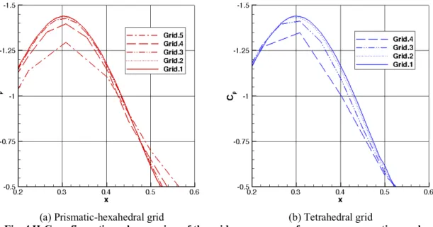
Table 5 summarizes various aspects of solution convergence on both grids, such as, the number of nonlinear iterations and the CPU time needed to achieve nonlinear solution convergence. Additionally, the table also shows the total number of search directions and the total number of preconditioner G-S iterations en route to the nonlinear solution convergence. For both grids, the HANIM-30_org solver converges in the least number of nonlinear iterations and encounters the fewest GCR failures, as expected. However, it also uses the greatest number of search directions, and preconditioner G-S iterations resulting in the consumption of the highest CPU time. Comparatively, the HANIM-30 solver needs an increased number of nonlinear iterations and encounters more GCR failures, but uses a significantly smaller number of search directions, as well as preconditioner G-S iterations. The HANIM-30 solver needs the least amount of time to solution. The HANIM-30 CPU time is half of the HANIM-30_org CPU time. Relative to the two HANIM solvers with a maximum of 30 search directions, HANIM-1 uses many more nonlinear iterations and encounters many more GCR failures.
For HANIM-1, the total number of preconditioner G-S iterations is comparable or less than that for HANIM-30. Conversely, the HANIM-1 CPU time to solution is slightly higher than the corresponding time for HANIM-30. For the fine grid, HANIM-1 uses about five million fewer meanflow G-S iterations (and 2.7 million fewer SA G-S iterations), but requires about 16,000 more CPU hours to achieve nonlinear solution convergence, as compared to the corresponding time for the HANIM-30 solver. The preconditioner is the innermost kernel of the solution methodology and generally the total number of G-S iterations provides a good measure of the solution efficiency from the CPU time standpoint. The apparent discrepancy between the CPU time and the number of preconditioner G-S iterations observed on the fine grid can be reconciled if the computational expense related to the evaluation of the nonlinear residuals and Jacobian is accounted for. The total number of nonlinear residual evaluations in a HANIM solver can be estimated as the sum of nonlinear iterations and search directions. This estimate assumes that the nonlinear control seldom fails. The number of Jacobian evaluations is estimated to be equal to the number of nonlinear iterations. Using these estimates, we can deduce from Table 5 that for the fine grid, HANIM-1 performs about 500,000 more nonlinear residual and Jacobian evaluations each, as compared to HANIM-30.
Table 5 Solution convergence statistics for two tetrahedral grids around the OM6 wing. Grid Nonlinear iterations CPU time, hours GCR search directions GCR failures G-S iterations, meanflow G-S iterations, SA model HANIM-1 coarse 40,010 860 52,051 12,039 875,845 295,765 HANIM-30_org 13,542 1,110 58,281 512 1,382,915 1,041,805 HANIM-30 16,157 581 35,944 4,692 734,595 340,800 HANIM-1 fine 707,288 126,834 920,187 212,833 9,223,710 8,549,755 HANIM-30_org 161,807 215,766 1,532,221 2,800 32,222,795 49,707,575 HANIM-30 264,513 110,986 843,645 79,384 14,342,390 12,287,850
12
IV. Results A. Benchmark Turbulent Flow Cases and GridsThe accuracy, scalability, and efficiency of the parallel mixed-element USM3D are assessed on two benchmark 3D configurations, namely, an H-C configuration and the OM6 wing. For a 3D H-C configuration, two families of prismatic-hexahedral and tetrahedral grids have been generated using a set of Fortran programs available at the TMR website under the “Cases and Grids for Turbulence Model Numerical Analysis” section, “3D Hemisphere Cylinder (new)” subsection. The grid-generation program is described in Ref. [18]. Both grid families have cylinder and hemisphere diameters of unity. The outflow boundary condition is assigned at a plane that is orthogonal to the cylinder axis and contains the cylinder base located at 𝑥 = 10. The symmetry boundary condition is assigned at the vertical plane corresponding to 𝑦 = 0. The farfield boundary is a quadrant of a sphere ((𝑥 − 10)J+ 𝑦J+ 𝑧J= 𝑟J, 𝑥 ≤ 10,
𝑦 ≥ 0) with the radius 𝑟 = 100. The finest-grid target near-wall spacing corresponds to y+ = 0.5, for the Reynolds number of 0.35´106 based on the sphere diameter. The finest prismatic-hexahedral grid in the family has been generated using the following input parameters [18]: 512 elements along the cylinder axis, 128 elements from the hemisphere apex to its base, and 2,560 elements in the radial direction. This grid has eight times more cells then the finest prismatic-hexahedral grid used in the previous study [33]. The finest grid in the tetrahedral-grid family consists of 256 elements along the cylinder axis, 64 elements from the hemisphere apex to its base, and 1,280 elements in the radial direction. A grid-coarsening program (also available at the TMR website and described in Ref. [18]) is used to extract six nested coarser grids for each grid family. The coarsening program applies an isotropic coarsening in the extraction of coarser grids. The grid-generation and grid-coarsening programs provide some grid quality characteristics including minimum planarity of quadrilateral faces. There are two ways to divide a quadrilateral face into two triangular faces by inserting a diagonal edge. The quadrilateral face planarity is defined as the cosine of the maximum of the two angles between outward normals of the triangular faces from two different diagonal edges. The unit planarity corresponds to a perfectly planar quadrilateral face; negative planarity indicates a significantly folded quadrilateral face. Tables 6 and 7 provide statistics related to the H-C configuration prismatic-hexahedral and tetrahedral grids, respectively.
Table 6 Statistics for a family of prismatic-hexahedral grids for an H-C configuration.
Grid Tetrahedra Prisms Hexahedra Total cells Total nodes Face planarity (minimum value) 1 0 125,829,120 503,316,480 629,145,600 568,585,537 0.9999 2 0 15,728,640 62,914,560 78,643,200 71,368,353 0.9999 3 0 1,966,080 7,864,320 9,830,400 8,995,153 0.9999 4 0 245,760 983,040 1,228,800 1,143,081 0.9999 5 0 30,720 122,880 153,600 147,637 0.9999 6 0 3,840 15,360 19,200 19,683 0.9998 7 0 480 1,920 2,400 2,788 0.9998
Table 7 Statistics for a family of tetrahedral grids for an H-C configuration.
Grid Tetrahedra Prisms Hexahedra Total cells Total nodes Face planarity (minimum value) 1 424,673,280 0 0 424,673,280 71,368,353 N/A 2 53,084,160 0 0 53,084,160 8,995,153 N/A 3 6,635,520 0 0 6,635,520 1,143,081 N/A 4 829,440 0 0 829,440 147,637 N/A 5 103,680 0 0 103,680 19,683 N/A 6 12,960 0 0 12,960 2,788 N/A 7 1,620 0 0 1,620 441 N/A
For the OM6 wing, two families of prismatic-hexahedral and tetrahedral grids have been generated using a set of Fortran programs available at the TMR website under the “Cases and Grids for Turbulence Model Numerical Analysis” section, “3D ONERA M6 Wing” subsection. In both grid families, the root chord is 1.0, the approximate values for semispan is 1.47602, and the mean aerodynamic chord is 0.80167. The farfield boundary is a hemisphere
(𝑥J+ 𝑦J+ 𝑧J= 𝑟J, 𝑦 ≥ 0) with the radius 𝑟 = 100. The symmetry boundary condition is assigned at the
13
family, the finest grid target near-wall spacing corresponds to y+ = 0.5, for the Reynolds number of 14.6´106 based on unit root chord. The grid consists of 192 elements along the wing semispan, 64 elements across the rounded tip, and 704 elements in the radial direction. Using a grid-coarsening program (available at the TMR website) six nested isotropically-coarsened grids are extracted within each family. Tables 8 and 9 provide statistics for the OM6 wing prismatic-hexahedral and tetrahedral grids, respectively.
Table 8 Statistics for a family of prismatic-hexahedral grids for the OM6 wing.
Grid Tetrahedra Prisms Hexahedra Total cells Total nodes Face planarity (minimum value) 1 0 17,301,504 51,904,512 69,206,016 60,777,345 0.08675 2 0 2,162,688 6,488,064 8,650,752 7,625,153 0.06641 3 0 270,336 811,008 1,081,344 960,225 0.05549 4 0 33,792 101,376 135,168 121,841 0.04918 5 0 4,224 12,672 16,896 15,705 0.04319 6 0 528 1,584 2,112 2,093 0.20020 7 0 66 198 264 300 0.43877
Table 9 Statistics for a family of tetrahedral grids for the OM6 wing.
Grid Tetrahedra Prisms Hexahedra Total cells Total nodes Face planarity (minimum value) 1 363,331,584 0 0 363,331,584 60,777,345 N/A 2 45,416,448 0 0 45,416,448 7,625,153 N/A 3 5,677,056 0 0 5,677,056 960,225 N/A 4 709,632 0 0 709,632 121,841 N/A 5 88,704 0 0 88,704 15,705 N/A 6 11,088 0 0 11,088 2,093 N/A 7 1,386 0 0 1,386 300 N/A B. Accuracy
The mixed-element USM3D provides NASA TMR website reference solutions for several benchmark flows. The accuracy of a serial mixed-element USM3D has been previously verified for 2D benchmark flows [8]. In this section, the parallel mixed-element USM3D solutions are verified and validated based on grid convergence studies for two benchmark 3D flows around the H-C configuration and the OM6 wing. Reference [33] also includes accuracy assessment of an interim parallel mixed-element version for the same benchmark flows. New aspects reported here are: (1) an increased grid resolution for the H-C configuration provided by a new family of prismatic-hexahedral grids with the finest grid of 629 million cells, (2) new OM6 wing USM3D solutions on prismatic-hexahedral grids, and (3) OM6 wing skin-friction verification data.
1. Hemisphere-Cylinder (H-C) Configuration
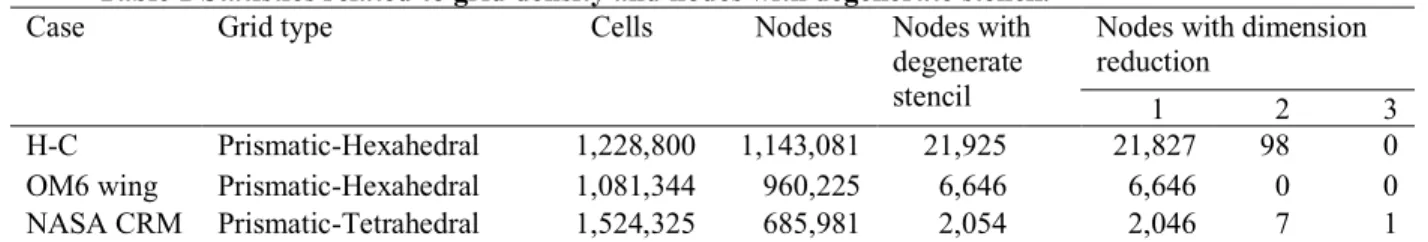
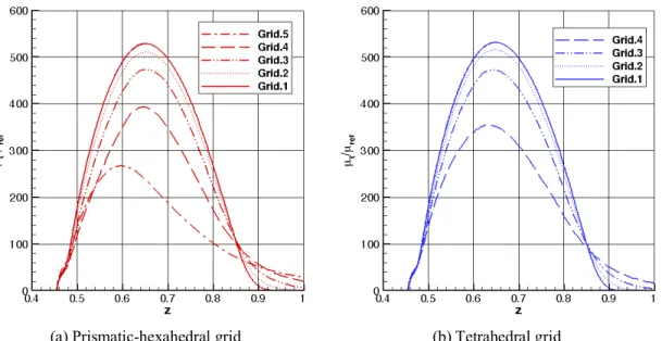
The 3D H-C solutions have been computed for a freestream Mach number of 0.6, an angle of attack of 19 degrees, and a Reynolds number of 0.35´106 based on the sphere diameter. Solutions are computed on the five finest prismatic-hexahedral grids (Grids 1-5 in Table 6) and the four finest tetrahedral grids (Grids 1-4 in Table 7). Grid convergence plots of lift, drag, and pitching-moment coefficients as well as the maximum eddy viscosity are presented in Fig. 2. The maximum eddy viscosity is nondimensionalized by 𝜇^mn, which is the laminar viscosity of the freestream flow.
In the plots, the abscissa represents a characteristic grid spacing, ℎ, that is computed as ℎ = 𝑁\5/g, where 𝑁 is the
number of cells in a given grid. All solution quantities converge in grid refinement for prismatic-hexahedral and tetrahedral grid families. Table 10 shows the aerodynamic coefficients and the maximum eddy viscosity in the finest grid solutions from the two grid families. Differences in various quantities are small. For the force coefficients, the maximum variation relative to the mean value is 0.25%. The variation relative to the mean value is 0.15% for the pitching moment and 0.57% for the maximum eddy viscosity.
In spite of the apparent monotonic convergence of aerodynamic coefficients in grid refinement (the only exception is the viscous-drag coefficient on the tetrahedral Grid 4) and close agreement of the aerodynamic quantities computed on the finest grids of the two families, extrapolation to the infinite-grid limit is problematic because no reliable order of convergence can be established. The convergence curves corresponding to the two different grid families cross and exhibit variability in the convexity on fine grids.
14
Table 10 H-C configuration: aerodynamic coefficients computed on the finest grids.
Family Total
lift Total drag Pressure drag Viscous drag Pitching moment eddy viscosity Maximum Prismatic-hexahedral 0.08620776 0.03465206 0.02209324 0.01255882 -0.02581175 1499.2611 Tetrahedral 0.08608755 0.03453019 0.02197932 0.01255087 -0.02573428 1516.3647
Grid convergence studies are based on a fundamental property that the accuracy of a RANS solution is determined by degrees of freedom. Thus, USM3D solutions on grids with a similar number of cells should be similar. In the present computations, a tetrahedral grid has 1.5 times fewer cells than the prismatic-hexahedral grid of the same level. The same tetrahedral grid has about 5 times more cells than the preceding-level prismatic-hexahedral grid (see Tables 6 and 7). Consequently, for an adequately grid-resolved solution, the difference between the aerodynamic coefficients computed on a tetrahedral grid and the prismatic-hexahedral grid of the same level should be significantly smaller than the difference between the aerodynamic coefficients computed on the tetrahedral grid and the preceding-level prismatic-hexahedral grid. This property seems to be satisfied for all grids and all quantities in Fig. 2.
(a) Total lift coefficient (b) Total drag coefficient
(c) Pressure drag coefficient (d) Viscous drag coefficient
15
(e) Pitching moment coefficient (f) Maximum eddy viscosity Fig. 2 Concluded.
To assess the grid topology effect on the accuracy of local solution characteristics, the solutions on the finest prismatic-hexahedral and tetrahedral grids (Grid 1) are compared. The global views of the surface pressure, skin-friction, and off-body solution distributions are presented in Fig. 3. Figure 3(a) shows the streamwise pressure distribution in the symmetry plane corresponding to 𝑦 = 0 and Fig. 3(b) shows the circumferential pressure distribution in the 𝑥 = 5.0 plane. The azimuth angle, 𝜑, is the abscissa in Fig. 3(b), that is computed as 𝜑 = cos\5u𝑧 v𝑦⁄ J+ 𝑥Jw. In the present computations, 𝜑 = 0° corresponds to the leeside (𝑦 = 0, 𝑧 > 0), 𝜑 = 90°
corresponds to the horizontal plane (𝑦 > 0, 𝑧 = 0), and 𝜑 = 180° corresponds to the windside, (𝑦 = 0, 𝑧 < 0). In the global views, the finest prismatic-hexahedral and tetrahedral grid solutions are indistinguishable. The computed pressure distributions qualitatively agree with the experimental data [34].
The tangential component of the skin friction, shown in Fig. 3(c), is computed as the projection of the skin friction vector on the tangential direction, which is defined on the hemisphere-cylinder surface as a unit vector tangential to the surface, normal to the x-direction, and pointing up (having a positive z-component). The tangential direction is uniquely defined almost everywhere on the surface, except at the symmetry plane. The tangential component of the skin friction is expected to change its sign at the crossflow-vortex separation and reattachment locations. The tangential skin-friction component in the 𝑥 = 5.0 plane indicates two crossflow vortices: the primary vortex rotating in the counterclockwise direction separates at 𝜑 ≈ 65°, the secondary vortex rotating clockwise separates at 𝜑 ≈ 30°
and reattaches at 𝜑 ≈ 42°. The tangential skin-friction distributions from the finest prismatic-hexahedral and tetrahedral grid solutions are almost indistinguishable in the global view of Fig. 3(c). A small difference is observed in the magnitude of the global minimum near 𝜑 = 15°. The minimum in the prismatic-hexahedral grid solution is somewhat deeper than the minimum computed in the tetrahedral grid solution.
A larger discrepancy is observed in the streamwise component of the skin friction shown in Fig. 3(d), especially downstream of the hemisphere-cylinder junction at 𝑥 ≈ 0.5 and on the leeside at 𝑥 ≈ 6.5, where the skin friction reflects the 3D effects of the crossflow vortices. Accurate representation of skin friction at these locations has been recognized as one of the challenges in the previous CFD code verification study [33]. Figures 3(e) and 3(f) show the off-body profiles of the horizontal crossstream velocity component and the eddy viscosity from the finest-grid solutions of the two grid families. The solution quantities are plotted along a vertical line attached to the upper surface of the cylinder at 𝑥 = 5.0 and 𝑦 = 0.21. The view is chosen to show the solution variation across the core of the primary crossflow vortex. The global views of the off-body solution profiles indicate that both grid families provide accurate solutions on the finest grids.
16
(a) Surface pressure in plane y=0 (b) Surface pressure in plane x=5.0
(c) Tangential skin friction in plane x=5.0 (d) Streamwise skin friction in plane y=0.0
(e) v-velocity along vertical line at x=5.0, y=0.21 (f) Eddy viscosity along vertical line at x=5.0, y=0.21 Fig. 3 H-C configuration: surface-pressure, skin-friction, and off-body solution components computed on the finest grids.
17
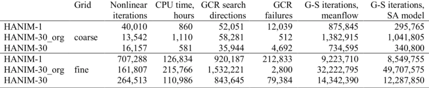
Closeup views are presented in Figs. 4-7 to examine the grid convergence of solutions in the vicinity of nontrivial flow features and in the region where the largest differences are observed in the finest-grid solutions presented in Fig. 3. Figure 4 illustrates local grid convergence of the leeside surface pressure around the suction peak. For both grid families, the pressure profiles computed on coarse grids are qualitatively similar to those computed on fine grids. The suction-peak location is accurately identified within the grid resolution. The relative difference between the minimum-pressure values from the coarsest- and the finest-grid solutions is less than 20%. The minimum-pressure profiles on the two finest grids (Grid 1 and Grid 2) are almost identical in the closeup view, especially for the prismatic-hexahedral grid family.
(a) Prismatic-hexahedral grid (b) Tetrahedral grid
Fig. 4 H-C configuration: closeup view of the grid convergence of pressure near suction peak.
Figure 5 shows a closeup view of the grid convergence of the streamwise component of the leeside skin friction coefficient at 𝑥 ≈ 6.5, the location where the largest discrepancy between the finest-grid (Grid 1) solutions is observed in the global view (see Fig. 3(d)). Large differences are observed between the coarse- and fine-grid solutions. The two coarsest-grid solutions in each family do not show any local minimum, whereas, finer-grid solutions show a progressively-pronounced local minimum. The significant differences between the solutions on the finest grids of the two families indicate that a better grid resolution is needed to accurately predict the 3D effects of crossflow vortices in the skin-friction variations for the region examined.
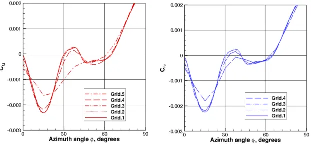
Figure 6 presents a closeup view for the grid convergence of the tangential component of the skin friction in the
𝑥 = 5.0 plane. Only the leeside surface is shown, 0° ≤ 𝜑 ≤ 90°, because solutions from all grids overplot on the windside surface, 90° < 𝜑 ≤ 180°. In the plots, two coarsest-grid curves are clearly distinguishable from the finer grid curves. Two finest grid curves are hardly distinguishable. Solutions on all grids indicate the primary vortex separation in the range of 𝜑 ≈ 60° to 𝜑 ≈ 70°. Only the coarsest grid solutions fail to recognize the separation and the reattachment of the secondary vortex, solutions on all other grids predict similar separation and reattachment locations.