Implied Volatility String Dynamics
∗
Matthias R. Fengler
†, Wolfgang K. H¨
ardle
CASE – Center for Applied Statistics and EconomicsHumboldt-Universit¨at zu Berlin, Spandauer Straße 1, 10178 Berlin, Germany
Enno Mammen
Department of Economics, University of Mannheim L 7, 3–5, 68131 Mannheim, Germany
December 8, 2003
∗We gratefully acknowledge financial support by the Deutsche Forschungsgemeinschaft and the
Sonder-forschungsbereich 373 “Quantifikation und Simulation ¨okonomischer Prozesse”.
Implied Volatility String Dynamics
Abstract
A primary goal in modelling the dynamics of implied volatility surfaces (IVS) aims at reducing complexity. For this purpose one fits the IVS each day and applies a prin-cipal component analysis using a functional norm. This approach, however, neglects the degenerated string structure of the implied volatility data and may result in a severe modelling bias. We propose a dynamic semiparametric factor model, which ap-proximates the IVS in a finite dimensional function space. The key feature is that we
only fit in thelocalneighborhood of the design points. Our approach is a combination
of methods from functional principal component analysis and backfitting techniques for additive models. The model is found to have an approximate 10% better perfor-mance than the typical na¨ıve trader models. The model can be a backbone in risk management serving for value at risk computations and scenario analysis.
JEL classification codes: C14, G12
Keywords: Implied Volatility Surface, Smile, Generalized Additive Models, Backfitting, Functional Principal Component Analysis
1
Introduction
Successful trading, hedging and risk managing of option portfolios crucially depends on the accuracy of the underlying pricing models. Departing from the pioneering foundations of op-tion theory laid by Black and Scholes (1973), Merton (1973) and Harrison and Kreps (1979), new valuation approaches are continuously developed and existing models are refined. How-ever, despite these pervasive developments, the model of Black and Scholes (1973) remains the pivot in modern financial theory and the benchmark for sophisticated models, be it from a theoretical or practical point of view.
The popularity of the Black and Scholes (BS) model is likely due to its clear and easy-to-communicate set of assumptions. Based on the geometric Brownian motion for the under-lying asset price dynamics, and continuous trading in a complete and frictionless market, simple closed form solutions for plain vanilla calls and puts are derived: given the current underlying price St at time t, the option’s strike price K, its expiry date T the prevailing
riskless interest rate rt, and an estimate of the (expected) market volatilityσ, option prices
are straightforward to compute.
The crucial parameter in option valuation by BS is the market volatility σ. Since it is unknown, one studies implied volatility ˆσ. Implied volatility is derived by inverting the BS formula for a cross section of options with different strikes and maturities traded at the same point in time. As is visible in the left panel of Figure 1 for May 2, 2000 (i.e. 20000502, a notation we will use from now on), implied volatilities display a remarkable curvature across the rescaled strike dimension moneynessκ, which is also called ‘smile’ or ‘smirk’, and – albeit to a lesser degree – a term structure across time to maturity τ, which fluctuates through time t. This dependence, captured by the function ˆσt : (κ, τ) →σˆt(κ, τ), is called
implied volatility surface (IVS). Apparently, it is in contrast with the BS framework in which volatility is assumed to be a constant across strikes, time to maturity and time.
There is a considerable amount of literature which aims at reconciling this empirical antag-onism with financial theory. Generally, this may be achieved by including another degree of freedom into option pricing models. Well known examples are stochastic volatility models, (Hull and White; 1987; Stein and Stein; 1991; Heston; 1993), models with jump diffusions, Bates (1996), or models building on general L´evy processes, e.g. based on the inverse Gaus-sian, Barndorff-Nielsen (1997), and generalized hyperbolic distribution, Eberlein and Prause (2002). These approaches capture the smile and term structure phenomena and the com-plexity of its dynamics to some extent, Tompkins (2001). For the case of deterministic local volatility models Dumas et al. (1998) documented in an extensive study time inconsistency for a number of parametric volatility functions.
[Figure 1 about here.]
[Figure 2 about here.]
A new interpretation of the inaccuracy of the advanced models asserts that option markets due to their depth and liquidity behave more and more self-governed: apart from the under-lying asset price dynamics, they are additionally driven by demand and supply conditions acting in options markets. In a comprehensive study Bakshi et al. (2000) show that a sig-nificant proportion of changes in option prices can neither be attributed to classical option pricing theory nor to market micro structure frictions. From this point of view, one inter-prets the IVS as a ‘state variable’, i.e. as an additional financial indicator, ruling in option markets, that reflects in an instantaneous and forward-looking manner the current state of
the market and the dynamics of its evolution. Thus, refined statistical model building of the IVS determines vitally the accuracy of applications in trading and risk-management.
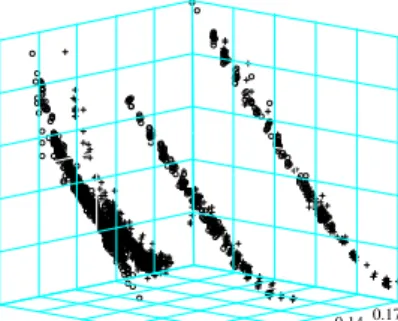
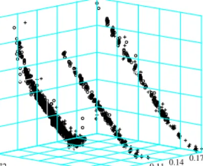
In modelling the IVS one faces two main challenges. First, the data design is degenerated: due to trading conventions, observations of the IVS occur only for a small number of ma-turities such as 1, 2, 3, 6, 9, 12, 18, and 24 months to expiry on issuance. Consequently, implied volatilities appear in a row like pearls strung on a necklace, Figure 1, or, in short: as ‘strings’. This pattern is also visible in the right panel of Figure 1, which plots the data design as seen from top. Options belonging to the same string have a common time to maturity. As time passes, the strings move through the maturity axis towards expiry while changing levels and shape in a random fashion. Second, also in the moneyness dimension, the observation grid does not cover the desired estimation grid at any point in time with the same density. Thus, even when the data sets are huge, for a large number of cases implied volatility observations are missing for certain sub-regions of the desired estimation grid. This is particularly virulent when transaction based data is used.
For the semi- or nonparametric approximations to the IVS that recently have been pro-moted by A¨ıt-Sahalia and Lo (1998); Rosenberg (2000); A¨ıt-Sahalia et al. (2001b); Cont and da Fonseca (2002); Fengler et al. (2003); Fengler and Wang (2003), this design may pose difficulties. For illustration, consider in Figure 2 (left panel) the fit of a standard Nadaraya-Watson estimator. Bandwidths are h1 = 0.03 for the moneyness and h2 = 0.04 for the time to maturity dimension (measured in years). The fit appears very rough, and there are huge holes in the surface, since the bandwidths are too small to ‘bridge’ the gaps between the maturity strings. In order to remedy this deficiency one would need to strongly increase bandwidths which may induce a large bias. Moreover, since the design is time-varying, bandwidths would also need to be adjusted anew for each trading day, which complicates
daily applications. Parametric models, e.g. as in Shimko (1993), An´e and Geman (1999), and Tompkins (1999) among others, are less affected by these data limitations, but seem to offer too little functional flexibility to capture the salient features of IVS patterns. Thus, parametric estimates may as well be biased.
In this paper we provide a new principal component approach for modelling the IVS: the complex dynamic structure of the IVS is captured by a low dimensional semiparametric factor model with time-varying coefficients. The IVS is approximated by unknown basis functions moving in a finite dimensional function space. The dynamics can be understood by using vector autoregression (VAR) techniques on the time-varying coefficients. Contrary to earlier studies, we will use only finite dimensional fits to implied volatilities which are obtained in
thelocalneighborhood of strikes and maturities, for which implied volatilities are recorded at
the specific day. Also, surface estimation anddimension reduction is achieved in one single step, not in two as is currently standard. Our technology can be seen as a combination of functional principal component analysis, nonparametric curve estimation and backfitting for additive models.
Let us denote the (ln)-implied volatility by Yi,j, where the index i is the number of the day
(i= 1, ..., I), and j = 1, ..., Ji is an intra-day numbering of the option traded on day i. The
observations Yi,j are regressed on two dimensional covariables Xi,j that contain moneyness
κi,j and maturity τi,j. Moneyness is defined as κi,j = Ki,j/Ft,i,j, i.e. strike Ki,j divided by
the underlying futures price Ft,i,j at time ti,j. We also considered the one-dimensional case
in which Xi,j =κi,j. However, since modelling the entire surface is more interesting, we will
m0(Xi,j) + L
X
l=1
βi,lml(Xi,j), (1)
where ml are smooth basis functions (l = 0, . . . , L). The IVS is approximated by a weighted
sum of smooth functions ml with weights βi,l depending on time i. The factor loadingβi
def =
(βi,1, . . . βi,L)> forms an unobserved multivariate time series. By fitting model (1), to the
implied volatility strings we obtain approximationsβbi. We argue that VAR estimation based
on βbi is asymptotically equivalent to estimation based on the unobserved βi. A justification
for this is given in Fengler et al. (2004) where the relations to Kalman filtering are discussed.
Lower dimensional approximations of the IVS based on principal components analysis (PCA) have been used in Avellaneda and Zhu (1997) and Fengler et al. (2002) in an application to the term structure of implied volatilities, and in Skiadopoulos et al. (1999) and Alexander (2001) in studies across strikes. Fengler et al. (2003) use a common principal components approach to study several maturity groups across the IVS simultaneously, while Cont and da Fonseca (2002) propose a functional PCA perspective for the IVS. All these approaches treat the IVS as a stationary process, and do not take particular care for the degenerated string structure which is apparent in Figure 1.
Our modelling approach is also different in the following respect: for instance, in Cont and da Fonseca (2002) the IVS is fitted on a grid for each day. Afterwards a PCA using a functional norm is applied to the surfaces. This treatment follows the usual functional PCA approach as described in Ramsay and Silverman (1997). In our approach the IVS is fitted each day at the observed design points Xi,j. This leads to a minimization with respect to
functional norms that depend on time i. We loose a nice feature of usual functional PCA though: when fitting the data forLand L∗ =L+ 1, the linear space spanned bymb0, . . . ,mbL
may not be contained in the one spanned by mb∗0, . . . ,mb∗L∗. On the other hand we only make
use of values of the implied volatilities at regions where they are observed. This avoids bias effects caused by global daily fits used in standard functional PCA’s.
The model can be employed in several respects: given the estimated functions mbl and the
time series βb, scenario simulations of potential IVS scenarios are straightforward. They can
help to give a more accurate assessment of market risk than previous approaches. Worst case scenarios can be identified, which provide additional supervision tools to risk managers. For trading, the model may be used as a tool of short range IVS prediction. Even when it is difficult to predict the levels of the IVS due to the behavior of the level dynamics likely close to a unit root, certain specific distortions of the IVS may be predictable. To traders the model offers a unified tool for volatility hedging of complex option positions.
Since this model delivers a dynamic description of the IVS and certain IVS strings it may also serve as a way to model state price density (SPD) dynamics: according to Breeden and Litzenberger (1978) the SPD can be derived as the second derivative of the price function of plain vanilla options. Since the data is sparse in strikes, an approach due to Shimko (1993) converts option prices into implied volatilities, fits the smile on a dense grid, and computes the option prices via BS. The derivative, numerically much more stable than before, is computed with respect to the price function now obtained. Thus, IVS dynamics can be converted into SPD dynamics, and exploited for pricing and trading such as in A¨ıt-Sahalia et al. (2001b) and Blaskowitz et al. (2003).
The paper is organized as follows: in the following section implied volatilities are described and the semiparametric factor model is introduced. In Section 3 the model is applied to DAX option implied volatilities for the sample period 1998 to May 2001. Further model
extensions and modifications are discussed in the conclusion.
2
Time-dependent implied volatility modelling
2.1
The semi-parametric factor model
Implied volatilities are derived from the BS option pricing formula for European calls and puts, Black and Scholes (1973). European style calls and puts are contingent claims on an asset St (paying no dividends for simplicity, here), which yield for strike K the pay-off
max(St−K,0) and max(K−St,0), respectively, at a given expiry day T. The asset price
process Stin the BS model is given by a geometric Brownian motion. The BS option pricing
formula for calls is given by:
CtBS(St, K, τ, r, σ) = StΦ(d1)−Ke−rτΦ(d2), (2)
where d1 =
ln(St/K)+(r+12σ2)τ
σ√τ and d2 =d1−σ
√
τ. Φ(u) denotes the cumulative distribution function of the standard normal distribution, τ = T −t time to maturity of the option, r
the riskless interest rate over the option’s life time, and σ the diffusion coefficient of the Brownian motion. Put prices Pt are obtained via the put-call-parityCt−Pt =St−e−τ rK.
The only unknown parameter in (2) is volatilityσ. Given observed market prices ˜Ct, implied
volatility ˆσ is defined by:
CtBS(St, K, τ, r,σˆ)−C˜t= 0 . (3)
Due to monotonicity of the BS price in the volatility parameter σ there exists a unique solution ˆσ >0. Define the moneyness metric κt=K/Ft, where Ft denotes the future price
In the dynamic factor model, we regress Yi,j
def
= ln{σˆi,j(κ, τ)} on Xi,j = (κi,j, τi,j) via
non-parametric methods. We work with log-implied volatility data, since the data appears less skewed and potential outliers are scaled down after taking logs. This is common practice in the IVS literature, see e.g. Avellaneda and Zhu (1997); Cont and da Fonseca (2002). In order to estimate the nonparametric components ml and the state variables βi,l in (1), we
borrow ideas from fitting additive models as in Stone (1986); Hastie and Tibshirani (1990); Horowitz et al. (2002). Our research is related to functional coefficient models such as Cai et al. (2000). Other semi- and nonparametric factor models include Connor and Linton (2000); Gouri´eroux and Jasiak (2001); Fan et al. (2003); Linton et al. (2003b). Nonparametric tech-niques are now broadly used in option pricing, e.g. Broadie et al. (2000); A¨ıt-Sahalia et al. (2001a); A¨ıt-Sahalia and Duarte (2003), and interest rate modelling, e.g. A¨ıt-Sahalia (1996); Ghysels and Ng (1989); Linton et al. (2003a).
Estimatesmbl, (l = 0, . . . , L) andβbi,l (i= 1, . . . , I; l = 1, . . . , L) are defined as minimizers
of the following least squares criterion (βbi,0
def = 1): I X i=1 Ji X j=1 Z ( Yi,j − L X l=0 b βi,lmbl(u) )2 Kh(u−Xi,j)du. (4)
Here,Khdenotes a two-dimensional product kernel,Kh(u) =kh1(u1)×kh2(u2), h= (h1, h2)
based on a one-dimensional kernel kh(v) =h−1k(h−1v).
In (4) the minimization runs over all functions mbl : R2 → R and all values βbi,l ∈ R. For illustration let us consider the case L = 0 : implied volatilities Yi,j are approximated by a
surface mb0 that does not depend on time i. In this degenerated case, mb0(u) = P
i,jKh(u−
Xi,j)Yi,j/Pi,jKh(u−Xi,j), which is the Nadaraya-Watson estimate based on the pooled
sample of all days. Note that in the algorithmic implementation of (4) the integral is replaced by Riemann sums on a fine grid.
Using (4) the implied volatility surfaces are approximated by surfaces moving in an L -dimensional affine function space {mb0+PLl=1αlmbl: α1, . . . , αL∈R}.The estimates mbl are
not uniquely defined: they can be replaced by functions that span the same affine space. In order to respond to this problem, we select mbl such that they are orthogonal.
Replacing in (4)mblbymbl+δgwith arbitrary functionsg and taking derivatives with respect
to δ yields for 0≤l0 ≤L I X i=1 Ji X j=1 ( Yi,j − L X l=0 b βi,lmbl(u) ) b βi,l0Kh(u−Xi,j) = 0. (5)
Furthermore, by replacing βbi,l by βbi,l+δ in (4) and again taking derivatives with respect
to δ, we get for 1 ≤l0 ≤L and 1≤i≤I
Ji X j=1 Z ( Yi,j − L X l=0 b βi,lmbl(u) ) b ml0(u)Kh(u−Xi,j) du= 0. (6)
Introducing the following notation for 1 ≤i≤I
b pi(u) = 1 Ji Ji X j=1 Kh(u−Xi,j), (7) b qi(u) = 1 Ji Ji X j=1 Kh(u−Xi,j)Yi,j, (8)
we obtain from (5)-(6) for 1≤l0 ≤L,1≤i≤I:
I X i=1 Jiβbi,l0 b qi(u) = I X i=1 Ji L X l=0 b βi,l0βbi,l b pi(u)mbl(u), (9) Z b qi(u)mbl0(u)du = L X l=0 b βi,l Z b pi(u)mbl0(u)mbl(u) du. (10)
We calculate the estimates by iterative use of (9) and (10). We start by initial values βb
(0)
i,l
constant on time intervals I1, . . . , IL. This means for l = 1, .., L put βb
(0)
i,l = 1 (for i ∈ Il),
and βb
(0)
i,l = 0 (for i /∈ Il). Here I1, ..., IL are pairwise disjoint subsets of {1, ..., I} and L
S
l=1
Il
is a strict subset of {1, ..., I}. For r ≥ 0 we put βb
(r)
i,0 = 1. Define the matrix B
(r)(u) by its elements: B(r)(u)l,l0 def = I X i=1 Jiβb (r−1) i,l0 βb (r−1) i,l bpi(u), 0≤l, l 0 ≤ L , (11)
and introduce a vector Q(r)(u) with elements
Q(r)(u)l def = I X i=1 Jiβb (r−1) i,l qbi(u), 0≤l ≤L . (12)
In the r-th iteration the estimate mb = (mb0, ...,mbL)
> is given by
b
m(r)(u) =B(r)(u)−1Q(r)(u). (13)
This update step is motivated by (9). The values of βb are updated in the r-th cycle as
follows: define the matrix M(r)(i)
M(r)(i)l,l0 def = Z b pi(u)mb (r) l0 (u) b m(lr)(u)du , 1≤l, l0 ≤L , (14)
and define a vector S(r)(i)
S(r)(i)l def = Z b qi(u)mbl(u) du− Z b pi(u)mb (r) 0 (u)mb (r) l (u) du , 1≤l ≤L . (15) Motivated by (10), put b βi,(r1), ...,βb (r) i,L > =M(r)(i)−1S(r)(i). (16)
The algorithm is run until only minor changes occur. In the implementation, we choose a grid of points and calculate mbl at these points. In the calculation ofM(r)(i) and S(r)(i), we
replace the integral by a Riemann integral approximation using the values of the integrated functions at the grid points.
As discussed above, mbl and βbi,l are not uniquely defined. Therefore, we orthogonolize b m0, . . . ,mbL in L 2(ˆp), where ˆp(u) = I−1PI i=1pˆi(u), such that PI i=1βbi,21 is maximal, and given βbi,1,mb0,mb1, PI
i=1βbi,22 is maximal, and so forth. These aims can be achieved by the
following two steps: first replace
b m0 by mb new 0 = mb0−γ >Γ−1 b m, b m by mbnew = Γ−1/2m,b b βi,1 .. . b βi,L by b βnew i,1 .. . b βnew i,L = Γ1/2 b βi,1 .. . b βi,L + Γ−1γ , (17) where mb = (mb1, . . . ,mbL) >
and the (L×L) matrix Γ = R b
m(u)mb(u)>pˆ(u)du, or for clar-ity, Γ = (Γl,l0), with Γl,l0 = R
b
ml(u) mbl0(u)ˆp(u)du. Finally, we have γ = (γl), with γl = R
b
m0(u)mbl(u)ˆp(u)du.
Note that by applying (17), mb0 is replaced by a function that minimizes
R b
m20(u)ˆp(u)du.
This is evident because mb0 is orthogonal to the linear space spanned by mb1, . . .mbL. By the
second equation of (17), mb1, . . . ,mbL are replaced by orthonormal functions in L
2(ˆp).
In a second step, we proceed as in PCA and define a matrix B with Bl,l0 =PI
i=1βbi,lβbi,l0 and calculate the eigenvalues of B, λ1 > . . . > λL, and the corresponding eigenvectors z1, . . . zL.
Put Z = (z1, . . . , zL). Replace
b
m by mbnew
(i.e. mbnew l =zl>mb),and b βi,1 .. . b βi,L by b βnew i,1 .. . b βnew i,L = Z> b βi,1 .. . b βi,L . (19)
After application of (18) and (19) the orthonormal basis mb1, . . . ,mbL is chosen such that PI
i=1βb 2
i,1 is maximal, and– given βbi,1, b m0,mb1 – the quantity PI i=1βb 2 i,2 is maximal, . . ., i.e. b
m1 is chosen such that as much as possible is explained by βbi,1 b
m1. Next mb2 is chosen to
achieve maximum explanation by βbi,1 b
m1+βbi,2 b
m2, and so forth.
The functions mbl are not eigenfunctions of an operator as in usual functional PCA. This is
because we use a different norm, namely R f2(u)ˆpi(u)du, for each day. Through the norming
procedure the functions are chosen as eigenfunctions in an L-dimensional approximating lin-ear space. The L-dimensional approximating spaces are not necessarily nested for increasing
L. For this reason the estimates cannot be calculated by an iterative procedure that starts by fitting a model with one component, and that uses the old L−1 components in the iteration step from L−1 toLto fit the next component. The calculation of mb0, . . . ,mbLhas
to be fully redone for different choices of L.
2.2
Choice of
L
,
h
, and speed of convergence
For the choice of L, we consider the residual sum of squares for different L:
RV(L)def= PI i PJi j n
Yi,j −PLl=0βbi,lmbl(Xi,j) o2 PI i PJi j (Yi,j −Y¯)2 , (20)
where ¯Y denotes the overall mean of the observations. The quantity 1−RV(L) is the portion of variance explained in the approximation, and Lcan be increased until a sufficiently high
level of fitting accuracy is achieved. This is a common selection method also in ordinary PCA.
For a data-driven choice of bandwidths, we propose an approach based on a weighted Akaike Information Criterion (AIC). We argue for using a weighted criterion, since the distribution of observations is very unequal, as was seen from Figure 5. To our experience, this leads to nonconvexity in the criterion and typically to inacceptably small bandwidths, see Fengler et al. (2003) for a first description of this problem. Given the unequal distribution of observa-tions, it is natural to punish the criterion in areas where the distribution is sparse. For a given weight function w, consider:
∆(m0, . . . , mL) def = E 1 N X i,j {Yi,j− L X l=0
βi,lml(Xi,j)}2w(Xi,j), (21)
for functionsm0, . . . , mL. The expectation operator is denoted byE. We choose bandwidths
such that ∆(mb0, . . . ,mbL) is minimal. According to the AIC this is asymptotically equivalent
to minimizing: ΞAIC1 def = 1 N X i,j {Yi,j − L X l=0 b βi,lmbl(Xi,j)} 2w(X i,j) exp 2L NKh(0) Z w(u)du . (22)
Alternatively, one may consider the computationally more easy criterion:
ΞAIC2 def = 1 N X i,j {Yi,j− L X l=0 b βi,lmbl(Xi,j)} 2 exp 2L NKh(0) R w(u)du R w(u)p(u)du . (23)
Putting w(u)def= 1, delivers the common AIC. This, however, does not take into account the quality of the estimation at the boundary regions or in regions where data is sparse, since in these regions p(u) is small. We propose to choose
w(u)def= 1
which gives equal weight everywhere as can be seen by the following considerations: ∆(m0, . . . , mL) = E 1 N X i,j ε2w(Xi,j) + E 1 N X i,j " L X l=0
βi,l{ml(Xi,j)−mbl(Xi,j)} #2 w(Xi,j) ≈ σ2 Z w(u)p(u)du + 1 N X i,j Z " L X l=0 βi,l{ml(u)−mbl(u)} #2 w(u)p(u)du . (25)
The two criteria become:
ΞAIC1 def = 1 N X i,j {Yi,j− L X l=0 b βi,lmbl(Xi,j)} 2 ˆ p(Xi,j) exp 2L NKh(0) Z 1 ˆ p(u)du , (26) and ΞAIC2 def = 1 N X i,j {Yi,j− L X l=0 b βi,lmbl(Xi,j)} 2 exp 2L NKh(0)µ −1 λ Z 1 ˆ p(u)du , (27)
where µλ denotes the Lebesgue measure of the design set.
Under some regularity conditions, the AIC is an asymptotically unbiased estimate of the mean averaged square error (MASE). In our setting it would be consistent if the density of
Xi,j did not depend on day i. Due to the irregular design, this is an unrealistic assumption.
For this reason, ΞAIC1 and ΞAIC2 estimate a weighted versions of MASE.
In our AIC the penalty term does not punish for the number parameters βbi,l that are
em-ployed to model the time series. This can be neglected because we will use a finite dimensional model for the dynamics of βi,l. The corresponding penalty term is negligible compared to
the smoothing penalty term. A corrected penalty term that takes care of the parametric model of βbi,j will be considered in Section 3.3 where the prediction performance is assessed.
Clearly the choice of h and L are not independent. From this point of view, one may think about minimizing (26) or (27) over both parameters. However, our practical experience shows that for a given L, changes in the criteria from variation in h is small, compared to variation in L for a givenh. To reduce the computational burden, we use (20) to determine model size L, and then (26) and (27) to optimize h for a given L.
Convergence of the iterations is measured by
Qk(r) def = I X i=1 Z L X l=0 b βi(r)mbl(r)(u)−βb (r−1) i mb (r−1) l (u) k du . (28)
As above (r) denotes the result from the rth cycle of the estimation. Here, we approximate the integral by a simple sum over the estimation grid. Putting k = 1,2, we have an L1 and anL2 measure of convergence. Iterations are stopped whenQ
k(r)≤kfor some small >0.
3
Applications
3.1
Data description and preparation
The data set under consideration contains tick statistics on the DAX future and DAX index options and was provided by the German-Swiss Futures Exchange EUREX for the period from January 1998 to May 2001. Both future and option data are contract based data, i.e. each single contract is registered together with its price, contract size, and time of settlement up to a hundredth second. Interest rate data in daily frequency, i.e. 1, 3, 6, 12 months FIBOR rates for the years 1998–1999 and EURIBOR rates for the period 2000– 2001, were obtained from Thomson Financial Datastream. Interest rate data was linearly interpolated to approximate a ‘riskless’ interest rate for the option specific time to maturity.
In order to avoid German tax bias, option raw data has undergone a preparation scheme which is due to Hafner and Wallmeier (2001) and described in the following. The entire data set is stored in the Financial Database MD*base,www.mdtech.de, maintained at CASE – Center for Applied Statistics and Economics, Berlin.
In a first step, we recover the DAX index values. To this end, we group to each option price observation Ht the future price Ft of the nearest available future contract, which was
traded within a one minute interval around the observed option. The future price observation was taken from the most heavily traded futures contract on the particular day, usually the 3 months contract. The no-arbitrage price of the underlying index in a frictionless market without dividends is given by St = Fte−rTF ,t(TF−t), where St and Ft denote the index and
the future price respectively, TF the future’s maturity date, and rT,t the interest rate with
maturity T −t.
The DAX index is a capital weighted performance index (Deutsche B¨orse; 2002), i.e. divi-dends less corporate tax are reinvested into the index. Therefore, at a first glance, dividend payments should have no or almost little impact on index options. However, when only the interest rate discounted future is used to recover implied volatilities from an inversion of the BS formula, implied volatilities of calls and puts can differ significantly. This discrepancy is especially large during spring when most of the 30 companies listed in the DAX distribute dividends. The point is best visible in Figure 3 from 20000404: implied volatilities of calls (crosses) and puts (circles) fall apart, thus violating the put-call-parity and general market efficiency considerations.
[Figure 4 about here.]
Hafner and Wallmeier (2001) argue that the marginal investor’s individual tax scheme is different from the one actually assumed to compute the DAX index. Consequently, the net dividend for this investor can be higher or lower than the one used for the index computation. This discrepancy, which the authors call ‘difference dividend’, has the same impact as a dividend payment for an unprotected option, i.e. it drives a wedge into the option prices and hence into implied volatilities. Denote by ∆Dt,T the time T value of this difference
dividend incurred between tand T. Consider the dividend adjusted futures pricing formula:
Ft =SterF(TF−t)−∆Dt,TF, (29)
and the dividend adjusted put-call parity:
Ct−Pt =St−∆Dt,THe
−rH(TH−t)−Ke−rH(TH−t) (30)
with TH denoting the call’sCt and the put’s Pt maturity date. Inserting equation (29) into
(30) yields Ct−Pt=Fte−rF(TF−t)+ ∆Dt,TH,TF −Ke −rH(TH−t), (31) where ∆Dt,TH,TF def = ∆Dt,TFe −rF(TF−t)−∆D t,THe
−rH(TH−t) is the desired difference dividend.
The ‘adjusted’ index level
˜
St=Fte−rF(TF−t)+ ∆Dt,TH,TF (32)
is that index level, which ties put and call implied volatilities exactly to the same levels when used in the inversion of the BS formula.
For an estimate of ∆ ˆDt,TH,TF, pairs of puts and calls of the strikes and same maturity are identified provided they were traded within a five minutes interval. For each pair the
∆Dt,TH,TF is derived from equation (31). To ensure robustness ∆ ˆDt,TH,TF is estimated by the median of all ∆Dt,TH,TF of the pairs for a given maturity at day t. Implied volatilities are recovered by inverting the BS formula using the corrected index value ˜St = Fte−rF(TF−t)+
∆ ˆDt,TH,TF. Note that ∆Dt,TH,TF = 0, when TH = TF. Indeed, when calculated also in this case, ∆ ˆDt,TH,TF proved to be very small (compared with the index value), which supports the validity of this approach. The described procedure is applied on a daily basis throughout the entire data set from 199801 to 200105.
In Figure 4, also from 20000404, we present the data after correcting the discounted future price with an implied difference dividend ∆ ˆDt= (10.3,5.0,1.9)>, where the first entry refers
to 16 days, the second to 45 days and the third to 73 days to maturity. Implied volatilities of puts and calls converge two one single string, while the concavity of the put volatility smile is remedied, too. Note that the overall level of implied volatility string is not altered through that procedure.
Since the data is transaction based and may contain potential misprints or outliers, a filter is applied: observations with implied volatility less than 4% and bigger than 80% are dropped. Furthermore, we disregard all observations having a maturity τ ≤ 10 days. After this filtering, the entire number of observations is more than 4.48 million contracts, i.e. is around 5 200 observations per day. All computations have been made with XploRe, www.i-xplore.de.
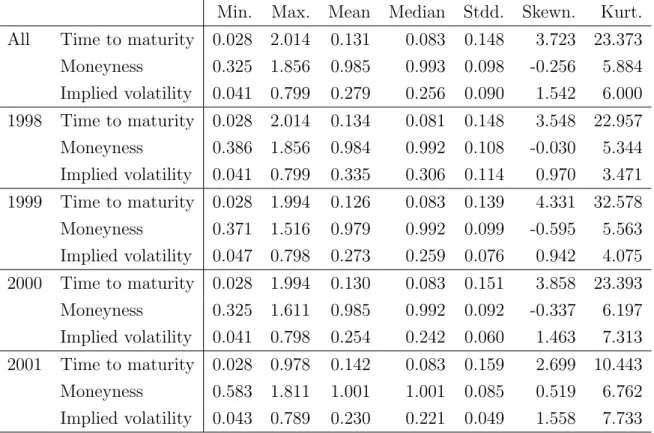
Table 1 gives a short summary of our IVS data. Most heavy trading occurs in short term contracts, as is seen from the difference between median and mean of the term structure distribution of observations as well as from its skewness. Median time to maturity is 30 days (0.083 years). Across moneyness the distribution is slightly negatively skewed. Mean implied volatility over the sample period is 27.9%.
[Table 1 about here.]
3.2
Implied Volatility Surface Modelling
Implied volatilities are observed only at particular strings, but it is common practice to think about them as being the observed structures of an entire surface, the IVS. This becomes evident, when one likes to price and hedge options with intermediate maturities. We model ln-implied volatility on Xi,j = (κi,j, τi,j)>. The grid covers in moneyness κ∈[0.80,1.20] and
in time to maturity τ ∈[0.05,0.5] measured in years.
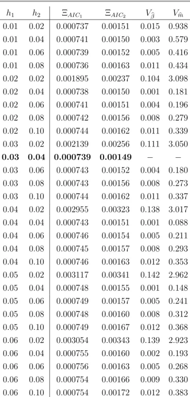
In this model, we employL= 3 basis functions, which capture around 96.0% of the variations in the IVS. We believe this to be of sufficiently high accuracy. Bandwidths used areh1 = 0.03 for moneyness and h2 = 0.04 for time to maturity. This choice is justified by Table 4 which presents estimates for the two AIC criteria. Both criterion functions become very flat near the minimum, especially ΞAIC1. However, ΞAIC2 assumes its global minimum in the
neighborhood of h∗ = (0.03,0.04)>, which is why we opt for these bandwidths. In Table 4 we also display a measure of how factor loadings and basis functions change relative to the optimal bandwidth h∗. We compute:
Vβb(hk) = v u u t L X l=0
var{|βbi,l(hk)−βbi,l(h∗)|}, (33)
and Vmb(hk) = v u u t L X l=0 var{|mbl(u;hk)−mbl(u;h ∗)|}, (34)
where hk runs over the values given in Table 4, and var(x) denotes the variance of x. It
is seen that changes in mb are 10 to 100 times higher in magnitude than those for βb. This
[Table 2 about here.]
In being able to choose such small bandwidths, the strength of our modelling approach is demonstrated: the bandwidth in the time to maturity dimension is so small that in the fit of a particular day, data from contracts with two adjacent time to maturities do not enter together pbi(u) in (7) and qbi(u) in (8). In fact, for given u
0, the quantities
b
pi(u0) and qbi(u
0)
are zero most of the time, and only assume positive values for dates iwhen observations are in the local neighborhood of u0. The same applies to the moneyness dimension. Of course, during the entire observation period I, it is mandatory that observations for eachufor some dates i are made.
[Figure 5 about here.]
In Figure 5 we display the L1 and L2 measures of convergence. Convergence is achieved quickly. The iterations were stopped after 25 cycles, when the L2 was less than 10−5. Figures 6 to 8 display the functions mb1 to mb4 together with contour plots. We do not
display the invariant function mb0, since it essentially is the zero function of the affine space fitted by the data: both mean and median are zero up to 10−2 in magnitude. We believe this to be estimation error. The remaining functions exhibit a more interesting patterns:
b
m1 in Figure 6 is positive throughout, and mildly concave. There is little variability across the term structure. Since this function belongs to the weights with highest variance, we interpret it as the time dependent mean of the (log)-IVS, i.e. a shift effect.
[Figure 6 about here.]
[Figure 8 about here.]
Function mb2, depicted in Figure 7, changes sign around the at-the-money region, which implies that the smile deformation of the IVS is exacerbated or mitigated by this eigenfunc-tion. Hence we consider this function as a moneyness slope effect of the IVS. Finally, mb3 is positive for the very short term contracts, and negative for contracts with maturity longer than 0.1 years, Figure 8. Thus, a positive weight in βb3 lowers short term implied volatilities and increases long term implied volatilities: mb3 generates the term structure dynamics of the IVS, it provides a term structure slope effect.
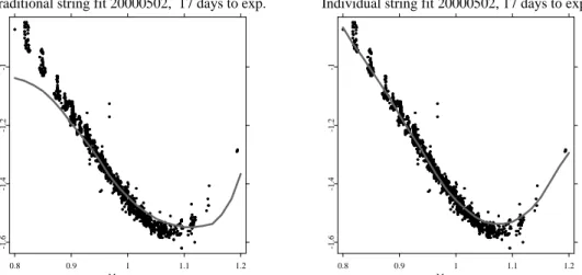
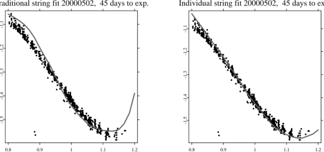
To appreciate the power of the semiparametric dynamic factor model, we inspect again the situation of 20000502. In Figure 9 we compare a Nadaraya-Watson estimator (left panel) with the semi-parametric factor model (right panel). In the first case, the bandwidths are increased to h= (0.06,0.25)> in order to remove all holes and excessive variation in the fit, while for the latter the bandwidths are kept ath = (0.03,0.04)>. While both fits look quite similar at a first glance, the differences are best visible when both cases are contrasted for each time to maturity string separately, Figures 10 to 13. Generally, the standard Nadaraya-Watson fit exhibits a strong directional bias, especially in the wings of the IVS. For instance, for the short maturity contracts, Figure 10, the estimated IVS is too low both in the OTM put and the OTM call region. At the same time, levels are too high for the 45 days to expiry contracts, Figure 11. For the 80 days to expiry case, Figure 12, the fit exhibits an S-formed shape, although the data lie almost on a linear line. Also the semi-parametric factor model is not entirely free of a directional bias, but clearly the fit is superior.
[Figure 10 about here.]
[Figure 11 about here.]
[Figure 12 about here.]
[Figure 13 about here.]
[Figure 14 about here.]
[Table 3 about here.]
[Table 4 about here.]
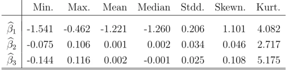
Figure 14 shows the entire time series of βb1 to βb3, summary statistics are given in Table 3
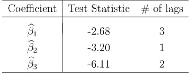
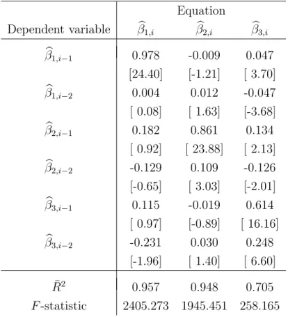
and contemporaneous correlation in Table 4. The correlograms given in the lower panel of Figure 14 display rich autoregressive dynamics of the factor loadings. The ADF tests at the 5% level, Table 5, indicate a unit root forβb1 andβb2. Thus, one may model first differences of the first two loading series together with the levels of βb3 in a parsimonious VAR framework. Alternatively, since the results are only marginally significant, one may estimate the levels of the loading series in a rich VAR model. We opt for the latter choice and use a VAR(2) model, Table 6. The estimation also includes a constant and two dummy variables, assuming the value one right at those days and one day after, when the corresponding IV observations of the minimum time to maturity string (10 days to expiry) were to be excluded from the estimation of the semiparametric factor model, confer Section 3.1. This is to capture possible seasonality effects introduced from the data filter.
Estimation results are displayed in Table 6. In the equations of βb1 and βb2 the constants
and dummies are weakly significant. However, for sake of clarity, estimation results on the constant and the dummy variables are not shown. As is seen all factor loadings follow AR(2) processes. There is also a number of remarkable cross dynamics: first order lags in the level dynamics, βb1, have a positive impact on the term structure, βb3. Second order lags in the term structure dynamics themselves influence positively the moneyness slope effect, βb2, and negatively the shift variable βb1: thus shocks in the the term structure may decrease the
level of the smile and aggravate the skew. Similar interpretations can be revealed from other significant coefficients in Table 6.
In earlier specifications of the model, we also included contemporaneous and lagged DAX returns into the regression equation. The results revealed a leverage interpretation of the first loading series, Black (1976): shocks in the underlying are negatively correlated with level changes in (implied) volatility, possibly due to a change in the debt-equity ratio. However, since for our horse-race in Section 3.3, we use a simple VAR without exogenous variables due to fairness, we do not show these results.
[Table 5 about here.]
[Table 6 about here.]
3.3
Prediction Performance
We now study the prediction performance of our model compared with a benchmark model. Model comparisons that have been conducted, for instance by Bakshi et al. (1997); Dumas et
al. (1998); Bates (2000); Jackwerth and Rubinstein (2001), often show that so called ‘na¨ıve trader models’ perform best or only little worse than more sophisticated models. These models used by professionals simply assert that today’s implied volatility is tomorrow’s implied volatility. There are two versions: the sticky strike assumption pretends that implied volatility is constant at fixed strikes. The sticky delta or sticky moneyness version claims this for implied volatilities observed at a fixed moneyness or option delta, Derman (1999). We use the sticky moneyness model as our benchmark. There are two reasons for this choice: first, from a methodological point of view, as has been shown by Balland (2002) and Daglish et al. (2003), the sticky strike rule as an assumption on the stochastic process governing implied volatilities, is not consistent with the existence of a smile. The sticky moneyness rule, however, can be. Second, practically, since we estimate our model in terms of moneyness, sticky moneyness rule is most natural.
Our methodology in comparing prediction performance is as follows: as presented in Sec-tion 3.2, the resulting times series of latent factors βbi,l is replaced by a times series model
with fitted values βei,l(ˆθ) based on βbi0,l with i0 ≤ i−1 ,1 ≤ l ≤ L, where ˆθ is a vector of
estimated coefficients seen in Table 6. Similarly to Section 2, we employ a AIC based on these fitted values as an asymptotically unbiased estimate of mean square prediction error.
For the model comparison we use criterion ΞAIC1 with w(u)
def
= 1. Additionally we penalize the dimension of the fitted time series model βe(θ):
e ΞAIC def = N−1 I X i Ji X j ( Yi,j− L X l=0 e βi,l(ˆθ)mbl(Xi,j) )2 ×exp 2 L NKh(0)µλ+ 2 dim(θ) N . (35)
and two dummy variables.
Criterion (35) is compared with the squared one-day prediction error of the sticky moneyness (StM) model: ΞStM def = N−1 I X i Ji X j (Yi,j−Yi−1,j0)2 . (36)
In practice, since one hardly observes Yi,j at the same moneyness as in i −1, Yi−1,j0 is
obtained via a localized interpolation of the previous day’s smile. Time to maturity effects are neglected, and observations, the previous values of which are lost due to expiry, are deleted from the sample.
Running the model comparison shows:
ΞStM = 0.00476
e
ΞAIC = 0.00439
Thus, the model comparison reveals that the semi-parametric factor model is approximate 10% better than the na¨ıve trader model. This is a substantial improvement given the high variance in implied volatility and financial data in general. An alternative approach would investigate the hedging performance of our model compared with other models, e.g. in following Engle and Rosenberg (2000). This is left for further research.
4
Conclusion and model extensions
In this study we present a modelling approach to the implied volatility surface (IVS) that takes care of the particular discrete string structure of implied volatility data. The technique
comes from functional PCA and backfitting in additive models. Unlike other studies, our ansatz is tailored to the degenerated design of implied volatility data by fitting basis functions in the local neighborhood of the design points only. We thus avoid bias effects.
Using transactions based DAX index implied volatility data from 1998 to May 2001, we recover a number of basis functions generating the dynamics of a single implied volatility string and surface. The functions may be intuitively interpreted as level, term structure and moneyness slope effects, and a term structure twist effect, known from earlier literature. We study the time series properties of parameters weights and complete the modelling approach by fitting vector autoregressive models. A three-dimensional VAR(2) describes IVS dynamics best.
Our modelling approach allows for a number of extensions that can be discussed. A first topic is efficiency. After the calculation of mb0, ...,mbL and βbi,1, ...,βbi,L the estimates of βi,l
may be replaced by the minimizers βei,1, ...,βei,L of
I X i=1 Ji X j=1 ( Yi,j − L X l=0 e βi,lmbl(Xi,j) )2 .
Discussions of other semiparametric models suggest that this estimate is more efficient than the estimate above. However, this approach has the disadvantage that it requires calculation of the components at all design points Xi,j.
Another extension would be to introduce into equation (4) weights wi,j. For instance, in
applications other than ours, the weights could correct for unequal values of Ji or could take
care of heteroscedastic errors, e.g. variances depending on maturity. Alternatively weights may be derived from economic variables such the underlying trading volume associated with a particular implied volatility observation.
A third modelling approach would be to replace (4) by I X i=1 Ji X j=1 I X k=1 Z ( Yi,j −mb0(u)− L X l=1 b βi,lmbl,k(u) )2 Kh(u−Xi,j)G(k−i)du,
where Gis a smooth function. In this case a system of principal components is fitted to the data that smoothly develops in time. In trading applications a model must be continuously updated and recalibrated. Thus in the trading context, this third model extension may be a fruitful starting point for even better exploiting the transaction based tick data.
Finally, as mentioned earlier, the semi-parametric model has a natural relation with Kalman filtering. Kalman filtering is a way to recursively find solutions to discrete-data linear filtering problems, Kalman (1960). For, writing our model more compactly as:
Θ(L)βi = ui (37)
Yi,j = m0(Xi,j) + L
X
l=1
βi,lml(Xi,j) +εi,j , (38)
where Θ(L)def= 1−θ1L−θ2L2. . .−θpLp denotes a polynomial of orderpin the lag operatorL,
we receive the typical state-space representation, where ui and εi,j is noise. Equation (38)
is called thestate equation depending on a parameter vector θ. It relates the (unobservable) state i of the system to the previous step i−1. The measurement equation (38) relates the state to the measurement, the IVS in our case. The difference to our work is that the time series modelling of βi is done afterrecovering it. For the integrated approach see Fengler et
References
A¨ıt-Sahalia, Y., 1996, Nonparametric pricing of interest rate derivative securities, Econo-metrica 64, 527–560.
A¨ıt-Sahalia, Y. and Duarte, J., 2003, Nonparametric option pricing under shape restrictions, Journal of Econometrics 116, 9–47.
A¨ıt-Sahalia, Y. and Lo, A., 1998, Nonparametric estimation of state-price densities implicit in financial asset prices, Journal of Finance 53, 499–548.
A¨ıt-Sahalia, Y., Bickel, P. J. and Stoker, T. M., 2001a, Goodness-of-fit tests for regression using kernel methods, Journal of Econometrics 105, 363–412.
A¨ıt-Sahalia, Y., Wang, Y. and Yared, F., 2001b, Do options markets correctly price the probabilities of movement of the underlying asset?, Journal of Econometrics 102, 67– 110.
Alexander, C., 2001, Principles of the skew, RISK 14(1), S29–S32.
An´e, T. and Geman, H., 1999, Stochastic volatility and transaction time: an activity-based volatility estimator, Journal of Risk 2(1), 57–69.
Avellaneda, M. and Zhu, Y., 1997, An E-ARCH model for the term-structure of implied volatility of FX options, Applied Mathematical Finance 4, 81–100.
Bakshi, G., Cao, C. and Chen, Z., 1997, Empirical performance of alternative option pricing models, Journal of Finance 52(5), 2003–2049.
Bakshi, G., Cao, C. and Chen, Z., 2000, Do call and underlying prices always move in the same direction?, Review of Financial Studies 13(3), 549–584.
Balland, P., 2002, Deterministic implied volatility models, Quantitative Finance 2, 31–44.
Barndorff-Nielsen, O. E., 1997, Normal inverse gaussian distributions and stochastic volatil-ity modelling, Scandinavian Journal of Statistics 24, 1–13.
Bates, D., 1996, Jumps and stochastic volatility: Exchange rate processes implicit in deutsche mark options, Review of Financial Studies 9, 69–107.
Bates, D. S., 2000, Post-’87 crash fears in the S&P 500 futures option market, Journal of Econometrics 94(1-2), 181–238.
Black, F., 1976, Studies of stock price volatility changes, Proceedings of the 1976 Meetings of the American Statistical Association, 177–181.
Black, F. and Scholes, M., 1973, The pricing of options and corporate liabilities, Journal of Political Economy 81, 637–654.
Blaskowitz, O., H¨ardle, W. and Schmidt, P., 2003, Skewness and kurtosis trades, Working paper, SfB 373, Humboldt-Universit¨at zu Berlin.
Breeden, D. and Litzenberger, R., 1978, Price of state-contingent claims implicit in options prices, Journal of Business 51, 621–651.
Broadie, M., Detemple, J. and Torr`es, O., 2000, American options with stochastics dividends and volatility: A nonparametric investigation, Journal of Econometrics 94, 53–92.
Cai, Z., Fan, J. and Yao, Q., 2000, Functional-coefficient regression models for nonlinear time series., Journal of the American Statistical Association 95, 941–956.
Connor, G. and Linton, O., 2000, Semiparametric estimation of a characteristic-based factor model of stock returns, Technical report.
Cont, R. and da Fonseca, J., 2002, The dynamics of implied volatility surfaces, Quantitative Finance 2(1), 45–60.
Daglish, T., Hull, J. C. and Suo, W., 2003, Volatility surfaces: Theory, rules of thumb, and empirical evidence, Working paper, J. L. Rotman School of Management, University of Toronto.
Derman, E., 1999, Regimes of volatility, RISK.
Deutsche B¨orse, 2002, Leitfaden zu den Aktienindizes der Deutschen B¨orse, 4.3 edn, Deutsche B¨orse AG.
Dumas, B., Fleming, J. and Whaley, R. E., 1998, Implied volatility functions: Empirical tests, Journal of Finance 80(6), 2059–2106.
Eberlein, E. and Prause, K., 2002, The generalized hyperbolic model: Financial derivatives and risk measures, in H. Geman, D. Madan, S. Pliska and T. Vorst (eds), Mathematical Finance - Bachelier Congress 2000, Springer Verlag, Heidelberg, New York, 245 – 267.
Engle, R. and Rosenberg, J., 2000, Testing the volatility term structure using option hedging criteria, Journal of Derivatives 8, 10–28.
Fan, J., Yao, Q. and Cai, Z., 2003, Adaptive varying-coefficient linear models, J. Roy. Statist. Soc. B. 65, 57–80.
Fengler, M. R. and Wang, Q., 2003, Fitting the smile revisited: A least squares kernel estimator for the implied volatility surface, SfB 373 Discussion Paper 2003-25, Humboldt-Universit¨at zu Berlin.
Fengler, M. R., H¨ardle, W. and Mammen, E., 2004, Semiparametric state space factor models, CASE Discussion Paper, Humboldt-Universit¨at zu Berlin.
Fengler, M. R., H¨ardle, W. and Schmidt, P., 2002, Common factors governing VDAX move-ments and the maximum loss, Journal of Financial Markets and Portfolio Management 16(1), 16–29.
Fengler, M. R., H¨ardle, W. and Villa, C., 2003, The dynamics of implied volatilities: A common principle components approach, Review of Derivatives Research 6, 179–202.
Ghysels, E. and Ng, S., 1989, A semiparametric factor model of interest rates and tests of the affine term structure, Review of Economics and Statistics 80, 535–548.
Gouri´eroux, C. and Jasiak, J., 2001, Dynamic factor models, Econometrics Review 20(4), 385–424.
Hafner, R. and Wallmeier, M., 2001, The dynamics of dax implied volatilities, International Quarterly Journal of Finance 1(1), 1–27.
H¨ardle, W., Klinke, S. and M¨uller, M., 2000, Xplore – Learning Guide, Springer Verlag, Heidelberg.
Harrison, J. and Kreps, D., 1979, Martingales and arbitrage in multiperiod securities mar-kets, Journal of Economic Theory 20, 381–408.
Hastie, T. and Tibshirani, R., 1990, Generalized additive models, Chapman and Hall, London.
Heston, S., 1993, A closed-form solution for options with stochastic volatility with applica-tions to bond and currency opapplica-tions, Review of Financial Studies 6, 327–343.
Horowitz, J., Klemela, J. and Mammen, E., 2002, Optimal estimation in additive models, Preprint.
Hull, J. and White, A., 1987, The pricing of options on assets with stochastic volatilities, Journal of Finance 42, 281–300.
Jackwerth, J. C. and Rubinstein, M., 2001, Recovering stochastic processes from option prices, Working paper, Universit¨at Konstanz.
Kalman, R. E., 1960, A new approach to linear filtering and prediction problems, Transac-tions of the ASME–Journal of Basic Engineering 82, 35–45.
Linton, O., Mammen, E., Nielsen, J. and Tanggaard, C., 2003a, Yield curve estimation by kernel smoothing, Journal of Econometrics. to appear.
Linton, O., Nguyen, T. and Jeffrey, A., 2003b, Nonparametric estimation of single factor Heath-Jarrow-Morton term structure models and a test for path independence, Technical report.
Merton, R. C., 1973, Theory of rational option pricing, Bell Journal of Economics and Management Science 4(Spring), 141–183.
Ramsay, J. O. and Silverman, B. W., 1997, Functional Data Analysis, Springer.
Rosenberg, J., 2000, Implied volatility functions: A reprise, Journal of Derivatives 7, 51–64.
Shimko, D., 1993, Bounds on probability, RISK 6, 33–37.
Skiadopoulos, G., Hodges, S. and Clewlow, L., 1999, The dynamics of the S&P 500 implied volatility surface, Review of Derivatives Research 3, 263–282.
Stein, E. M. and Stein, J. C., 1991, Stock price distributions with stochastic volatility: An analytic approach, Review of Financial Studies 4, 727–52.
Stone, C. J., 1986, The dimensionality reduction principle for generalized additive models, The Annals of Statistics 14, 592–606.
Tompkins, R., 1999, Implied volatility surfaces: Uncovering regularities for options on financial futures, Working paper, Vienna University of Technology.
Tompkins, R., 2001, Stock index futures markets: Stochastic volatility models and smiles, The Journal of Futures Markets 21(1), 43–78.
Min. Max. Mean Median Stdd. Skewn. Kurt. All Time to maturity 0.028 2.014 0.131 0.083 0.148 3.723 23.373 Moneyness 0.325 1.856 0.985 0.993 0.098 -0.256 5.884 Implied volatility 0.041 0.799 0.279 0.256 0.090 1.542 6.000 1998 Time to maturity 0.028 2.014 0.134 0.081 0.148 3.548 22.957 Moneyness 0.386 1.856 0.984 0.992 0.108 -0.030 5.344 Implied volatility 0.041 0.799 0.335 0.306 0.114 0.970 3.471 1999 Time to maturity 0.028 1.994 0.126 0.083 0.139 4.331 32.578 Moneyness 0.371 1.516 0.979 0.992 0.099 -0.595 5.563 Implied volatility 0.047 0.798 0.273 0.259 0.076 0.942 4.075 2000 Time to maturity 0.028 1.994 0.130 0.083 0.151 3.858 23.393 Moneyness 0.325 1.611 0.985 0.992 0.092 -0.337 6.197 Implied volatility 0.041 0.798 0.254 0.242 0.060 1.463 7.313 2001 Time to maturity 0.028 0.978 0.142 0.083 0.159 2.699 10.443 Moneyness 0.583 1.811 1.001 1.001 0.085 0.519 6.762 Implied volatility 0.043 0.789 0.230 0.221 0.049 1.558 7.733
Table 1: Summary statistics on the data base from 199801 to 200105 for the IVS application in Section 3.2, entirely and on an annual basis. 2001 is from 200101 to 200105, only.
h1 h2 ΞAIC1 ΞAIC2 Vβb Vmb 0.01 0.02 0.000737 0.00151 0.015 0.938 0.01 0.04 0.000741 0.00150 0.003 0.579 0.01 0.06 0.000739 0.00152 0.005 0.416 0.01 0.08 0.000736 0.00163 0.011 0.434 0.02 0.02 0.001895 0.00237 0.104 3.098 0.02 0.04 0.000738 0.00150 0.001 0.181 0.02 0.06 0.000741 0.00151 0.004 0.196 0.02 0.08 0.000742 0.00156 0.008 0.279 0.02 0.10 0.000744 0.00162 0.011 0.339 0.03 0.02 0.002139 0.00256 0.111 3.050 0.03 0.04 0.000739 0.00149 − − 0.03 0.06 0.000743 0.00152 0.004 0.180 0.03 0.08 0.000743 0.00156 0.008 0.273 0.03 0.10 0.000744 0.00162 0.011 0.337 0.04 0.02 0.002955 0.00323 0.138 3.017 0.04 0.04 0.000743 0.00151 0.001 0.088 0.04 0.06 0.000746 0.00154 0.005 0.211 0.04 0.08 0.000745 0.00157 0.008 0.293 0.04 0.10 0.000746 0.00163 0.012 0.353 0.05 0.02 0.003117 0.00341 0.142 2.962 0.05 0.04 0.000748 0.00155 0.001 0.148 0.05 0.06 0.000749 0.00157 0.005 0.241 0.05 0.08 0.000748 0.00160 0.008 0.312 0.05 0.10 0.000749 0.00167 0.012 0.368 0.06 0.02 0.003054 0.00343 0.139 2.923 0.06 0.04 0.000755 0.00160 0.002 0.193 0.06 0.06 0.000756 0.00163 0.005 0.268 0.06 0.08 0.000754 0.00166 0.009 0.330 0.06 0.10 0.000754 0.00172 0.012 0.383
Table 2: Bandwidth selection via AIC as given in (26) and (27) for different choices of h:
h1 refers to moneyness andh2 to time to maturity measured in years; the bandwidth chosen
Min. Max. Mean Median Stdd. Skewn. Kurt. b β1 -1.541 -0.462 -1.221 -1.260 0.206 1.101 4.082 b β2 -0.075 0.106 0.001 0.002 0.034 0.046 2.717 b β3 -0.144 0.116 0.002 -0.001 0.025 0.108 5.175
b β1 βb2 βb3 b β1 1 0.241 0.368 b β2 1 −0.003 b β3 1
Coefficient Test Statistic # of lags b β1 -2.68 3 b β2 -3.20 1 b β3 -6.11 2
Table 5: ADF tests onβb1 to βb3 for the full IVS model, intercept included in each case. Third
column gives the number of lags included in the ADF regression. For the choice of lag length, we started with four lags, and subsequently deleted lag terms, until the last lag term became significant at least at a 5% level. MacKinnon critical values for rejecting the hypothesis of a unit root are -2.87 at 5% significance level, and -3.44 at 1% significance level.
Equation Dependent variable βb1,i βb2,i βb3,i b β1,i−1 0.978 -0.009 0.047 [24.40] [-1.21] [ 3.70] b β1,i−2 0.004 0.012 -0.047 [ 0.08] [ 1.63] [-3.68] b β2,i−1 0.182 0.861 0.134 [ 0.92] [ 23.88] [ 2.13] b β2,i−2 -0.129 0.109 -0.126 [-0.65] [ 3.03] [-2.01] b β3,i−1 0.115 -0.019 0.614 [ 0.97] [-0.89] [ 16.16] b β3,i−2 -0.231 0.030 0.248 [-1.96] [ 1.40] [ 6.60] ¯ R2 0.957 0.948 0.705 F-statistic 2405.273 1945.451 258.165
Table 6: Estimation results of an VAR(2) of the factor loadings βbi. t-statistics given in
brackets, R¯2 denotes the adjusted coefficient of determination. The estimation includes an
intercept and two dummy variables (both not shown), which assume the value one right at those days and one day after, when the corresponding IV observations of the minimum time to maturity string (10 days to expiry) were to be excluded from the estimation of the semiparametric factor model.
List of Figures
1 Left panel: call and put implied volatilities observed on 2nd May, 2000. Right
panel: data design on 2nd May, 2000, ODAX. . . 44
2 Nadaraya-Watson estimator and semi-parametric factor model fit for 20000502.
Bandwidths for both estimates h1 = 0.03 for the moneyness and h2 = 0.04for
the time to maturity dimension. . . 45
3 IVS ticks on April 4, 2000, derived from future prices that are interest rate
discounted only. Put implied volatility are circles, call implied volatility crosses. 46
4 IVS ticks on April 4, 2000, derived from future prices that are interest rate
discounted and corrected with the implied difference dividend. Put implied
volatility are circles, call implied volatility crosses. . . 47
5 Left panel: convergence in the IVS models. Solid line shows the L1, the dotted
line the L2 measure of convergence. Total number of iterations is 25. Right
panel: average density pˆ(u) = I−1PI
i=1pˆi(u). Bandwidths are h1 = 0.03 for
moneyness and h2 = 0.04 for time to maturity. . . 48
6 Factor mb1 in the left panel (moneyness lower left axis). Right panel shows
contour plots of this function (moneyness left axis). Lines are thick for positive level values, thin for negative ones. The gray scale becomes increasingly lighter the higher the level in absolute value. Stepwidth between contour lines is 0.028,
estimated from ODAX data 199801-200105. . . 49
7 Factor mb2 in the left panel (moneyness lower left axis). Right panel shows
contour plots of this function (moneyness left axis). Lines are thick for positive level values, thin for negative ones. The gray scale becomes increasingly lighter the higher the level in absolute value. Stepwidth between contour lines is 0.225,
8 Factor mb3 in the left panel (moneyness lower left axis). Right panel shows
contour plots of this function (moneyness left axis). Lines are thick for positive level values, thin for negative ones. The gray scale becomes increasingly lighter the higher the level in absolute value. Stepwidth between contour lines is 0.240,
estimated from ODAX data 199801-200105. . . 51
9 Nadaraya-Watson estimator with h = (0.06,0.25)> and semi-parametric
fac-tor model with h= (0.03,0.04)> for 20000502. . . 52
10 Bias comparison of the Nadaraya-Watson estimator with h = (0.06,0.25)>
(left panel) and the semi-parametric factor model with h= (0.03,0.04)> (right
panel) for the 17 days to expiry data (black bullets) on 20000502. . . 53
11 Bias comparison of the Nadaraya-Watson estimator with h = (0.06,0.25)>
(left panel) and the semi-parametric factor model with h= (0.03,0.04)> (right
panel) for the 45 days to expiry data (black bullets) on 20000502. . . 54
12 Bias comparison of the Nadaraya-Watson estimator with h = (0.06,0.25)>
(left panel) and the semi-parametric factor model with h= (0.03,0.04)> (right
panel) for the 80 days to expiry data (black bullets) on 20000502. . . 55
13 Bias comparison of the Nadaraya-Watson estimator with h = (0.06,0.25)>
(left panel) and the semi-parametric factor model with h= (0.03,0.04)> (right
panel) for the 136 days to expiry data (black bullets) on 20000502. . . 56
14 Upper panel: time series of weights(βb1,βb2,βb3)>. Lower panel: autocorrelation
IVS Ticks 20000502 0.16 0.28 0.40 0.51 0.63 0.56 0.71 0.87 1.02 1.18 0.26 0.32 0.38 0.44 0.50 Data Design 0.4 0.5 0.6 0.7 0.8 0.9 1 1.1 1.2 1.3 1.4 Moneyness 0 0.1 0.2 0.3 0.4 0.5 0.6 0.7 Time to maturity
Figure 1: Left panel: call and put implied volatilities observed on 2nd May, 2000. Right panel: data design on 2nd May, 2000, ODAX.
Model fit 20000502 0.14 0.23 0.32 0.41 0.50 0.80 0.88 0.96 1.04 1.12 -1.46 -1.30 -1.14 -0.98 -0.82
Semiparametric factor model fit 20000502
0.14 0.23 0.32 0.41 0.50 0.80 0.88 0.96 1.04 1.12 -1.47 -1.31 -1.16 -1.00 -0.85
Figure 2: Nadaraya-Watson estimator and semi-parametric factor model fit for 20000502.
Bandwidths for both estimates h1 = 0.03 for the moneyness and h2 = 0.04 for the time to
Implied Volatility Surface Ticks 0.08 0.11 0.14 0.17 0.20 0.72 0.82 0.92 1.02 1.12 0.25 0.29 0.32 0.35 0.39
Figure 3: IVS ticks on April 4, 2000, derived from future prices that are interest rate dis-counted only. Put implied volatility are circles, call implied volatility crosses.
Implied Volatility Surface Ticks 0.08 0.11 0.14 0.17 0.20 0.72 0.82 0.92 1.02 1.12 0.26 0.29 0.33 0.36 0.40
Figure 4: IVS ticks on April 4, 2000, derived from future prices that are interest rate dis-counted and corrected with the implied difference dividend. Put implied volatility are circles, call implied volatility crosses.
5 10 15 20 25 Number of Iterations -4 -3 -2 -1 0 1 2 3 4 5 6 log_10(Fitting Criterion) Average density 0.14 0.23 0.32 0.41 0.50 0.80 0.88 0.96 1.04 1.12 11.75 23.36 34.96 46.56 58.16
Figure 5: Left panel: convergence in the IVS models. Solid line shows the L1, the dotted
line the L2 measure of convergence. Total number of iterations is 25. Right panel: average
density pˆ(u) = I−1PI
i=1pˆi(u). Bandwidths are h1 = 0.03 for moneyness and h2 = 0.04 for
0.14 0.23 0.32 0.41 0.50 0.80 0.88 0.96 1.04 1.12 0.70 0.84 0.99 1.14 1.28 0.89 1.00 1.10 1.20 0.16 0.27 0.38 0.50
Figure 6: Factor mb1 in the left panel (moneyness lower left axis). Right panel shows contour
plots of this function (moneyness left axis). Lines are thick for positive level values, thin for negative ones. The gray scale becomes increasingly lighter the higher the level in absolute value. Stepwidth between contour lines is 0.028, estimated from ODAX data 199801-200105.
0.14 0.23 0.32 0.41 0.50 0.80 0.88 0.96 1.04 1.12 -1.39 -0.36 0.67 1.70 2.73 0.89 1.00 1.10 1.20 0.16 0.27 0.38 0.50
Figure 7: Factor mb2 in the left panel (moneyness lower left axis). Right panel shows contour
plots of this function (moneyness left axis). Lines are thick for positive level values, thin for negative ones. The gray scale becomes increasingly lighter the higher the level in absolute value. Stepwidth between contour lines is 0.225, estimated from ODAX data 199801-200105.
0.14 0.23 0.32 0.41 0.50 0.80 0.88 0.96 1.04 1.12 -3.66 -2.15 -0.63 0.88 2.40 0.89 1.00 1.10 1.20 0.16 0.27 0.38 0.50
Figure 8: Factor mb3 in the left panel (moneyness lower left axis). Right panel shows contour
plots of this function (moneyness left axis). Lines are thick for positive level values, thin for negative ones. The gray scale becomes increasingly lighter the higher the level in absolute value. Stepwidth between contour lines is 0.240, estimated from ODAX data 199801-200105.
Model fit 20000502 0.14 0.23 0.32 0.41 0.50 0.80 0.88 0.96 1.04 1.12 -1.47 -1.31 -1.16 -1.00 -0.85
Semiparametric factor model fit 20000502
0.14 0.23 0.32 0.41 0.50 0.80 0.88 0.96 1.04 1.12 -1.47 -1.31 -1.16 -1.00 -0.85
Figure 9: Nadaraya-Watson estimator with h = (0.06,0.25)> and semi-parametric factor
Traditional string fit 20000502, 17 days to exp. 0.8 0.9 1 1.1 1.2 Moneyness -1.6 -1.4 -1.2 -1
Individual string fit 20000502, 17 days to exp.
0.8 0.9 1 1.1 1.2 Moneyness -1.6 -1.4 -1.2 -1
Figure 10: Bias comparison of the Nadaraya-Watson estimator with h = (0.06,0.25)> (left
panel) and the semi-parametric factor model with h = (0.03,0.04)> (right panel) for the 17
Traditional string fit 20000502, 45 days to exp. 0.8 0.9 1 1.1 1.2 Moneyness -1.5 -1.4 -1.3 -1.2 -1.1
Individual string fit 20000502, 45 days to exp.
0.8 0.9 1 1.1 1.2 Moneyness -1.5 -1.4 -1.3 -1.2 -1.1
Figure 11: Bias comparison of the Nadaraya-Watson estimator with h = (0.06,0.25)> (left
panel) and the semi-parametric factor model with h = (0.03,0.04)> (right panel) for the 45
Traditional string fit 20000502, 80 days to exp. 0.8 0.9 1 1.1 1.2 Moneyness -1.5 -1.4 -1.3 -1.2 -1.1
Individual string fit 20000502, 80 days to exp.
0.8 0.9 1 1.1 1.2 Moneyness -1.5 -1.4 -1.3 -1.2 -1.1
Figure 12: Bias comparison of the Nadaraya-Watson estimator with h = (0.06,0.25)> (left
panel) and the semi-parametric factor model with h = (0.03,0.04)> (right panel) for the 80
Traditional string fit 20000502, 136 days to exp. 0.8 0.9 1 1.1 1.2 Moneyness -1.6 -1.5 -1.4 -1.3 -1.2 -1.1
Individual string fit 20000502, 136 days to exp.
0.8 0.9 1 1.1 1.2 Moneyness -1.6 -1.5 -1.4 -1.3 -1.2 -1.1
Figure 13: Bias comparison of the Nadaraya-Watson estimator with h = (0.06,0.25)> (left
panel) and the semi-parametric factor model with h= (0.03,0.04)> (right panel) for the 136
basis coeff. 1 1998 1999 2000 2001 Time -1.5 -1 -0.5 basis coeff. 2 1998 1999 2000 2001 Time -0.05 0 0.05 0.1 basis coeff. 3 1998 1999 2000 2001 Time -0.1 -0.05 0 0.05 0.1
basis coeff. 1: ACF
0 5 10 15 20 25 30 lag 0 0.5 1 acf
basis coeff. 2: ACF
0 5 10 15 20 25 30 lag 0 0.5 1 acf
basis coeff. 3: ACF
0 5 10 15 20 25 30 lag 0 0.5 1 acf
Figure 14: Upper panel: time series of weights (βb1,βb2,βb3)>. Lower panel: autocorrelation