Numerical Investigation of Subsonic Flow through an Aggressive Flat Bottom Diffuser

University of Colorado, Boulder

CU Scholar

Aerospace Engineering Sciences Graduate Theses &

Dissertations

Aerospace Engineering Sciences

Summer 7-25-2014

Numerical Investigation of Subsonic Flow through

an Aggressive Flat Bottom Diffuser

Nicholas Alexander Mati

University of Colorado Boulder, [email protected]

Follow this and additional works at:

http://scholar.colorado.edu/asen_gradetds

Part of the

Aerospace Engineering Commons

This Thesis is brought to you for free and open access by Aerospace Engineering Sciences at CU Scholar. It has been accepted for inclusion in Aerospace Engineering Sciences Graduate Theses & Dissertations by an authorized administrator of CU Scholar. For more information, please contact

[email protected].

Recommended Citation

Mati, Nicholas Alexander, "Numerical Investigation of Subsonic Flow through an Aggressive Flat Bottom Diffuser" (2014).Aerospace Engineering Sciences Graduate Theses & Dissertations.Paper 1.

Numerical Investigation of Subsonic Flow through an

Aggressive Flat Bottom Diffuser

by

Nicholas Alexander Mati

A thesis submitted to the

Faculty of the of the Graduate School of the

University of Colorado in partial fulfillment

Of the requirement for the degree of

Master of Science

Department of Aerospace Engineering Sciences

2014

This thesis entitled:

Numerical Investigation of Subsonic Flow through an Aggressive Flat Bottom Diffuser

written by Nicholas Mati

has been approved for the Department of Aerospace Engineering Sciences

________________________________

Kenneth Jansen

________________________________

Alireza Doostan

Date

The final copy of this thesis has been examined by the signatories, and we

Find that both the content and the form meet acceptable presentation standards

Mati, Nicholas (Aerospace Engineering)

Numerical Investigation of Subsonic Flow through an Aggressive Flat Bottom Diffuser Thesis directed by Professor Kenneth Jansen

Airflow through an aggressive, constant pressure gradient, flat-bottomed 2D diffuser is simulated with the compressible version of the stabilized, implicit finite element code PHASTA. The freestream Mach number of fluid entering the diffuser is held at a value of with a PI feedback loop. For a quasi 1D flow, the expansion ratio of produces a Mach number of by the end of the diffuser or Aerodynamics Interface Plane (AIP). However, the compact geometry and high targeted pressure gradient of result in massive asymmetric separation off of the curved ceiling. To improve this situation, wall suction is applied to the ceiling, floor, and corners of the duct as a flow control surrogate while the geometry is iterated to better achieve the targeted pressure gradient.

After iterating geometry, the separation dynamics are studied in greater detail with both Unsteady Reynolds Averaged Navier Stokes (URANS) and Delayed Detached-Eddy Simulations (DDES). The duct naturally develops a strong vortical structure downstream of the AIP which can be limited to the upper half of the duct with corner suction. However, the structure of the secondary flow with just corner suction differs substantially between RANS and DDES. Experimental results are not yet available for comparison. Tangential blowing is also studied, but results are only available for flow control on the floor. RANS simulations indicate that floor blower is moderately more effective at maintaining steady, attached flow at the AIP than the floor suction used in other simulations.

Contents

Chapter

Chapter 1 Introduction ... 1

Chapter 2 Numerical Setup and Methodologies ... 3

2.1 Navier-Stokes Solver ... 3

2.2 Geometries and Boundary Conditions ... 4

2.2.1 Overview of experimental geometries ... 5

2.2.2 Overview of numerical geometries ... 7

2.2.3 Baseline boundary conditions... 8

2.2.4 Mach Control ... 11

2.2.5 Flow Control Surrogates ... 12

2.3 Mesh Generation ... 13

Chapter 3 Diffuser Design... 17

3.1 Pressure Gradient Design ... 17

3.2 Selection of Suction Velocities ... 19

3.3 Iteration of Initial Diffuser Curvature ... 22

Chapter 4 Separation Dynamics and Flow Control ... 25

4.1 No Blower Results ... 25

4.1.1 URANS and DDES with No Suction ... 25

4.1.2 RANS and DDES with Corner Suction ... 27

4.1.3 RANS with Full Surrogate Flow Control ... 29

4.2 Coandă Blowing ... 31

Chapter 5 Conclusions and Future Work ... 33

Tables

Table 1: Selected list of geometry configurations ... 8 Table 2: Effective Areas and Mass Flow Rates with and ... 21

Figures

Figure 1: S-duct studied by Wellborn et al. [1] ... 1

Figure 2: S-duct studied by Vaccario et al. [2] _{... 1}

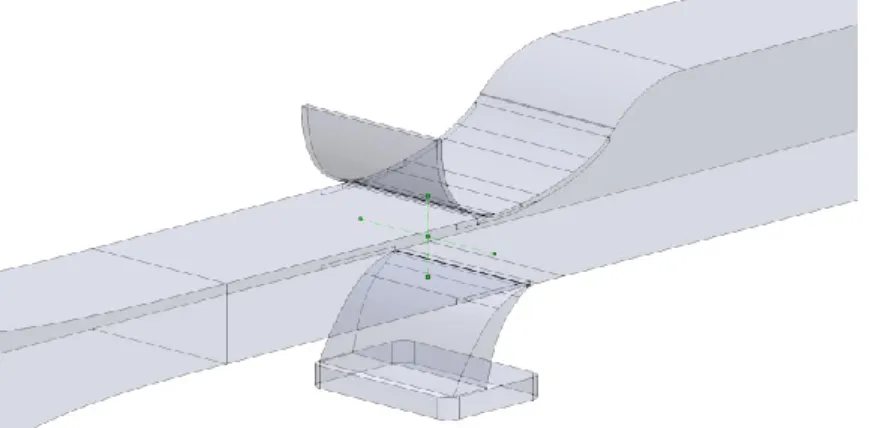
Figure 3: 3D Numerical Geometry including Upper and Lower Blower. The origin is located at the intersection of the green lines. ... 5

Figure 4: Overview of Experimental setup provided by the RPI experimental team [7]. ... 6

Figure 5: Experimental test section with honeycomb, upper blower, and AIP pressure rakes [7]_{. The lower blower is} not shown in this configuration. ... 7

Figure 6: 3D View of Diffuser and Suction Patches. ... 13

Figure 7: 2D profile of the diffuser examined in this work. The location of suction on the upper surface of the diffuser is shown in green and suction on the lower surface is shown in blue. Corner suction is shown in red. ... 13

Figure 8: of the First Node Off of the Wall. The picture is taken from a time averaged Series 12 simulation with no flow control activated. The first element height is uniformly . For this setup, . ... 14

Figure 9: Various mesh refinements used with upper and lower blowers. ... 15

Figure 10: Construction of Provided Geometry. The first 41% of the diffuser is approximated by two ellipses (solid black), followed by a set of splines (light green) and then an arc to maintain continuity at the AIP. ... 18

Figure 11: Geometry Shape and Upper Surface Slope of Series 1. ... 18

Figure 12: Expected Quasi-1D Pressure distribution of Series 1. The targeted pressure gradient is shown in red. .... 18

Figure 13: Velocity Contour of Instantaneous Flow field with and . ... 20

Figure 14: Velocity Contour of Instantaneous Flow field with and . ... 20

Figure 15: Velocity Contour of Instantaneous Flow field with and . ... 20

Figure 16: Velocity Contour of Instantaneous Flow field with and . ... 20

Figure 17: Velocity Contour of Time Averaged Flow over with and . .... 21

Figure 19: Ramp curvature and CFD pressure distribution on the original geometry. Yellow curvature combs are

shown with the geometry to the left... 22

Figure 20: Ramp curvature and CFD pressure distribution on an intermediate geometry after some iteration. The altered curvature of the new geometry is shown with green curvature combs. ... 23

Figure 21: Expected quasi-1D pressure distribution of Series 5. The targeted pressure gradient is shown in red... 23

Figure 22: Expected quasi-1D pressure distribution of Series 8. The targeted pressure gradient is shown in red... 23

Figure 23: Ramp curvature and CFD pressure distribution on the geometry which was sent for manufacturing. The altered curvature of the new geometry is shown with green curvature combs. ... 24

Figure 24: Streamlines and Velocity Contour of Baseline URANS Time Averaged Flow over . ... 26

Figure 25: Streamlines and Velocity Contour of Baseline DDES Time Averaged Flow over ... 26

Figure 26: Series 8 URANS No Suction Mach Contours. Results are averaged over 2400 time steps corresponding to an interval of . Dark isolines are drawn at increments... 26

Figure 27: Series 8 DDES No Suction Mach Contours. Results are averaged over 20000 time steps corresponding to an interval of . Isolines are drawn at increments. ... 27

Figure 28: : Streamlines and Contour of URANS with Corner Suction averaged over . ... 28

Figure 29: Streamlines and Contour of URANS with Corner Suction averaged over . ... 28

Figure 30: Velocity contour of DDES with Corner Suction Averaged over ... 28

Figure 31: Series 8 DDES Corner Suction Mach, Pressure, and Eddy Viscosity at the Centerline. Results are averaged over 20000 time steps corresponding to an interval of . Dark isolines are drawn at intervals of and . ... 28

Figure 32: Series 8 URANS Corner Suction Mach, Pressure, and Eddy Viscosity at the Centerline. Results are averaged over 2000 time steps corresponding to an interval of . Dark isolines are drawn at intervals of and . ... 29

Figure 33: Streamlines and Velocity Contour of Full Suction URANS Time Averaged Flow over . .. 30

Figure 34: Velocity projected onto the plane. ... 30

Figure 35: Series 8 URANS Full Suction Mach Contours. Results are averaged over . Dark isolines are drawn at increments. ... 30

Figure 37: Series 8 URANS RMS Streamwise Velocity fluctuations at the AIP. Results are averaged over . . 31 Figure 38: Series 12 URANS Mach Contours with Ceiling and Corner Suction. Results are averaged over 600 time steps corresponding to an interval of . Dark isolines are drawn at increments. ... 32 Figure 39: Series 12 URANS Mach Contours with Ceiling and Corner Suction plus Blowing on the Floor. Results are averaged over 600 time steps corresponding to an interval of . Dark isolines are drawn at

increments. ... 32 Figure 40: Series 12 RMS from URANS Full Suction ... 32

Chapter 1

Introduction

On most military aircraft and some civilian aircraft, turbojet or low bypass turbofan engines are mounted internally in the fuselage or wing. This necessitates the use of inlet ducts to create a flow path that connects the externally visible air intake with the engine compressor or fan. It is desirable to design the inlet duct to produce a uniform, steady flow with low total pressure loss and distortion at the Aerodynamic Interface Plane or AIP (i.e. the plane separating the compressor inlet from the duct). These qualities have the effect of making the engine less susceptible to compressor stall and increase the overall efficiency of the system. The inlet duct is also commonly used as a diffuser to convert kinetic energy of the incoming flow into elevated static pressure at the AIP. This increase in pressure drops the compression ratio required by the engine compressor to achieve a particular combustion chamber pressure and allows the compressor blades to be optimized for a smaller range of flow velocities.

In the last few decades, S-shaped diffusers such as those shown in Figure 1 and Figure 2 have received special attention. Geometric considerations are substantial driving factors; it is not uncommon for air intakes to be positioned on the side or bottom of an aircraft while the turbine is centered in the body.

Because the flow experiences an adverse pressure gradient as it approaches the AIP, diffusers tend to be susceptible to boundary layer separation. The S-ducts add to this problem by forcing the flow to navigate turns that further increase the adverse pressure gradient. To prevent the entropy production and loss of total pressure at the AIP inherent with separation, S-ducts tend to be fairly long with a gradual expansion to the full engine diameter. Unfortunately, the overall lengths of aircraft, especially UAVs, are typically constrained by the propulsion system length [2] which has led to increased emphasis on compact inlet design. To maintain attached flow under the high pressure gradients associated with very short S-ducts, flow control devices such as Coandă-type steady or pulsed injection, wall suction, or vortex generators are required. Blower and vortex generators have been used successfully on a number of circular and rectangular geometries [2] [3]_{, but most of the recent numerical and experimental flow}

control literature has examined ducts with aggressive turns.

Complex, nonlinear secondary flows in compact S-ducts tend to make the study of flow control devices difficult. Because of this, it is potentially useful to quantify the effects from flow control in a simplified geometry such as a low offset, compact diffusing S-duct. However, relatively little work exists for this particular geometry and the experimental work that does exist does not deal with active flow control. For example, Feakins et al. (reference [4]) merely examines the effect of downstream boundary conditions on a similar compact, asymmetric diffuser operating in an incompressible regime. A search of the literature has not yielded a thorough numeric investigation of flow control for a compact inlet duct operating in a subsonic compressible regime.

The present work partially fills this gap by numerically examining an aggressive flat bottom diffuser with a length to AIP height of , an area ratio of , and a targeted pressure gradient of . The diffuser is simulated using the stabilized, finite element Computational Fluid Dynamics (CFD) code PHASTA. Without any flow control, the aggressive geometry induces massive detachment on the upper surface of the duct which creates substantial distortion at the AIP and a total pressure loss in excess of . Wall suction is initially used as a flow control surrogate with mass flow rates of roughly on the top and on the bottom to maintain attached flow. Separation is most severe in the corners of the duct and required additional corner suction. Floor blowing with less than 1% total mass flow produces a similar effect as the floor suction with a total pressure loss of roughly 6%. Results are still pending for upper surface blowing.

Chapter 2

Numerical Setup and Methodologies

2.1

Navier-Stokes Solver

PHASTA (Parallel Hierarchic Adaptive Stabilized Transient Analysis) is a parallel, stabilized, predictor multi-corrector, implicit finite element CFD code. The compressible version of PHASTA discretizes the full set of

unsteady compressible Navier Stokes equations in conservative form. That is, it solves the system of equations given in (1) [_⏟ ] ([ ] [ ]) ⏟ ( [ ] [ ]) ⏟ (1)

where [ ] [ ] is the conservative variable vector1, is a vector of body forces and energy sinks/sources (which is usually neglected), ( ) is the viscous stress for a Newtonian fluid, and is heat conduction from Fourier’s law. Dotting eq. (1) with an arbitrary weight function and integrated by parts puts it into the weak form shown in eq. (2).

∫ ( ) ∫ ( ) (2)

To stabilize the method for advection dominated cases, the Streamline Upwind Petrov – Galerkin or SUPG term

̂ ( ( ) ( ) ) is added to the residual (where ̂ and is the Jacobian

). The residual is then discretized with a series of basis functions . Although PHASTA supports more complicated shape functions, linear tetrahedral elements are used in all following simulations due to load balancing

considerations. The second order accurate generalized- method is then used to perform the time stepping and GMRES is used to solve the linear algebra associated with an implicit method. More details may be found in reference [5].

1 _{In modern versions of PHASTA, the conservative state vector [}

] [ ] is replaced by the

primitive variable vector [ ] [ ] to make calculating the advective and diffusive fluxes, as wells

The Spalart Allmaras (SA) RANS turbulence model is applied in most simulations. It is a one equation turbulence model which uses the Boussinesq approximation ( ) (where (

) is the strain rate tensor) to model the Reynolds stresses [6]_{. The turbulent eddy viscosity is calculated from a}

transported quantity ̃ which is governed by the equation

̃ ̃ ̂ ̃ ( ̃ ) ( ( ( ̃) ̃ ) ̃ ̃ ) (3)

In eq. (3), is the distance to the wall; , , and are constants; and and ̂ are nonlinear functions2_{. More}

details may be found in references [6] and [7].

To better capture the unsteady separation off of the diffuser, large eddy simulation (LES) is desirable. However, the high Reynolds numbers on the order of ( ) in the test section make pure LES impractical. Instead, Delayed Detached-Eddy Simulation (DDES) is used. DDES can be interpreted as a hybrid RANS / LES turbulence model; it links the modeling of to the local mesh resolution with RANS being used on large elements close to the wall and LES being used on small elements further away from the wall. The implementation of DDES based off of the SA turbulence model is fairly simple with the distance in the wall destruction term (i.e. the second term on the RHS in eq. (3) ) being replaced by ̅ ( ) where ( ) is a characteristic element size,

is a constant, and is a function chosen to minimize modeled stress depletion caused by premature switching to LES in the boundary layer. More details are available in reference [8].

In PHASTA, the transport equation for ̃ is solved separately from the pressure, velocity, and temperature states. Primitive variables and eddy viscosity are alternately updated until the residual drops by about 3 orders of magnitude.

2.2

Geometries and Boundary Conditions

Several different configurations of the computational domain are considered in subsequent sections. The defining characteristics of these configurations include the presence or absence of an exit diffuser, the presence or absence of ceiling and/or floor blowers, and the profile of the test section diffuser. All simulated geometries

2 _{In the original version of the SA model (reference [7]) there are two extra terms involving a function}

which is used to make

̃ a stable solution within a small basin of attraction and a function which is used to artificially trip the boundary layer at

discussed in this text share the same test section area ratio of , length to AIP height of , and targeted pressure gradient of (or ) in the diffuser. The coordinate system is also

consistent between configurations with the -axis pointing in the streamwise direction towards the outlet, the -axis pointing up toward the curved portion of the diffuser, and the -axis completing the triad. The origin is located at the interface between the throat and the diffuser and is centered in the throat with respect to both the and -directions as shown in Figure 3.

Figure 3: 3D Numerical Geometry including Upper and Lower Blower. The origin is located at the intersection of the green lines.

The numeric simulations were conducted in conjunction with experiments at Rensselaer Polytechnic Institute (RPI). In general, CFD was able to iterate the flow path shape fairly rapidly and led or aided the diffuser and blower designs. The experimental team then manufactured the test section based on this CAD. Consequently, both the numeric and experimental results use identical flow paths to within manufacturing tolerance, material deflection, and discretization error.

2.2.1 Overview of experimental geometries

The numerical simulations tried to emulate the experimental setup as closely as possible. Consequently, limitations and design considerations of the experiment substantially influence several aspects of the CFD including geometric shape, boundary conditions, and instrumentation of the computational domain. Because of this, it is useful to first consider the experimental geometry.

The experiment is composed of a number of separate components. Moving from left to right in Figure 4, the blower, a Cincinnati Fan model HP-12G29 driven by a electric motor, is used to provide the primary flow.

The flow slows down as it passes through the blower diffuser resulting mean speeds of less than by the time it reaches the settling chamber. This diffuser is also used to transition to a rectangular cross section. The settling chamber is bounded by a set of screens which are intended to attenuate the turbulent kinetic energy in the inviscid core. From there, flow passes through a ( ) long contraction section with an area ratio of before entering the test section throat. The blower is controlled by a variable frequency drive which allows the volumetric flow rate to be adjusted as needed up to at standard conditions [8]_{. This corresponds to a maximum throat}

Mach number in excess of .

Figure 4: Overview of Experimental setup provided by the RPI experimental team [9]_.

The primary flow path in the test section consists of a ( ) long throat, a long quasi-constant pressure gradient diffuser, and a straight section which extends roughly behind the start of the diffuser. The throat has a uniform height of ( ) while the region downstream of the diffuser has a height of ( ) giving the diffuser an area ratio of . The entire test section has a uniform width of ( ).

The flow path is completely two dimensional in the test section with no variation of profile in the spanwise direction. Coupled with clear side and bottom walls, this makes PIV3 substantially easier to perform than it would be with multiple curved walls. Additionally, this two dimensionality (ideally) simplifies the flow and allows the effectiveness of flow control devices to be tested without the secondary flows off of a second, uncontrolled turn of previous S-ducts. Unfortunately, the rectangular cross section still results in intersecting boundary layers in the

3 _{PIV or particle image velocimetry is a flow visualization technique which uses optical cameras to track the motion of particles}

in the fluid stream. These particles are chosen to have a small Stokes number such that they closely follow fluid pathlines, thus enabling a reconstruction of the flow field.

corners with a corresponding increase in momentum loss. This predisposes the corners to flow reversal before other regions would normally separate. To mitigate this issue, fluid is extracted from corners through numerous small, choked holes in the side walls. The duct work connecting to these suction patches is visible in Figure 4. This thins the corner boundary layer and, from simulations, produces a more uniform baseline separation pattern.

Figure 5: Experimental test section with honeycomb, upper blower, and AIP pressure rakes [9]_{. The lower blower is not}

shown in this configuration.

Depending on the configuration, the floor, ceiling, and AIP of the duct are or will be heavily instrumented with static pressure ports and, in the case of the AIP, pressure rakes. The static pressure ports on the floor and ceiling have small diameter openings and relatively long response times making them better suited for determining mean pressure. However, the Kulite® _{pressure sensors used on the AIP pressure rakes have a much faster response time}

and are sampled at allowing large eddies and transient flow asymmetries to be resolved. Ports are also available roughly upstream of the start of the diffuser for a Kiel probe to measure the free stream Mach number. The CFD measures throat Mach number in the center of the duct at this streamwise location.

2.2.2 Overview of numerical geometries

Over the course of the project, the geometry changed for a number of different reasons making it somewhat difficult to generate a coherent and descriptive naming convention. Although it is possible to describe the major geometric features of a model, doing so quickly produces exceedingly long names, e.g. “the version 1 lower blower, exit diffuser, iteration 3 test diffuser geometry.” Instead, a numeric versioning system is used in all subsequent sections to categorize CFD geometry. The series number typically refers to major changes in geometry such as

altering the shape of the test section diffuser, including an exit diffuser, or including various blower geometry. Less substantial changes such as splitting faces on the CAD model are denoted by a subversion number. For example, 12.0 is the first iteration in series 12 which, from Table 1, uses a lower blower with the iteration 3 test section diffuser. However, subversion numbers are largely transparent in this document with only the most recent or applicable simulations results of a series being presented.

The first three entries in Table 1, i.e. series 1, 5, and 8, were created while iterating the diffuser shape. The sponsor provided the profile used in series 1 which was subsequently modified to produce series 5 and the final diffuser shape in series 8. All of the initial series are “clean” with no blower geometry; they instead rely on floor and ceiling suction to act as flow control surrogates and maintain attached flow. All geometries start at the interface between the settling chamber and the contraction section.

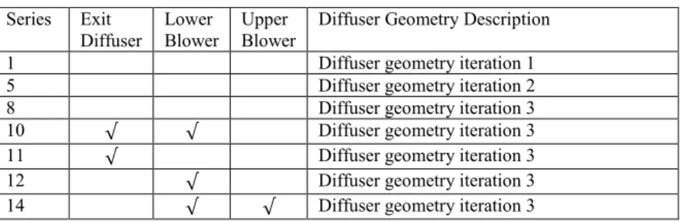
Table 1: Selected list of geometry configurations

Series Exit

Diffuser Lower Blower Upper Blower Diffuser Geometry Description

1 Diffuser geometry iteration 1

5 Diffuser geometry iteration 2

8 Diffuser geometry iteration 3

10 Diffuser geometry iteration 3

11 Diffuser geometry iteration 3

12 Diffuser geometry iteration 3

14 Diffuser geometry iteration 3

The diffuser profile from series 8 is used in series 10 through 14. Series 10 and 11 add an exit diffuser after the test section to more faithfully reproduce the experimental flow path. However, backflow at the outlet led to numeric difficulties and the exit diffusers were abandoned. Series 12 and 14 return to the non-diffusing outlets used in all other series. They also add a lower blower (series 12) or both upper and lower blowers (series 14).

2.2.3 Baseline boundary conditions

Simulations of the first few series (e.g. series 1, 5, and 8) use grandfathered temperature boundary conditions originating in a prior computational study [3]. In particular, a uniform temperature of is applied at the inlet and

is applied on all duct walls. At the outlet, a zero heat flux (HF) BC is prescribed which leaves the temperature there floating in a manner similar to a Neumann BC. While the outlet HF BC closely approximates reality, Chen does not clearly describe in his dissertation how the inlet and wall temperatures are derived [3]_{; he instead just asserts}

that the wall temperature is “calculated given the freestream Mach number [in the duct throat] … and the contraction ratio of 100” [3] _{without providing further details. These boundary condition likely exceed what they should be by}

between 4 and 8%, but were kept in the first few series to only study the effects of changing diffuser geometry. More representative temperature BCs may be calculated using isentropic flow arguments. When run with a throat Mach number of and attached flow in the diffuser, the series 8.2 contraction section total pressure sits at roughly . Assuming that the blower isentropically compresses air from an ambient reference temperature of and pressure of to the contraction inlet pressure, the resulting inlet temperature becomes:

( )

( )

(4)

All simulations after series 9 use this temperature for inlets and isothermal walls. As with earlier series, the outlet receives a zero heat flux BC.

It should be noted that the constant inlet temperature and isothermal walls are not particularly good

approximations. When the diffuser separates, the pressure recovery drops substantially and increases the contraction inlet pressure. For example, DDES runs in series 8 with no flow control yield inlet pressures near . Isentropic compression to this pressure corresponds to a temperature of . Further, there are real world losses in the blower which further increase the temperature. The walls are also not isothermal. At , the isentropic core drops to roughly while dissipative losses in the boundary layer produce higher temperatures and create large temperature gradients. It is speculated that these gradients may dominate the heat transfer on the outside of the test section making zero heat flux BCs on no slip walls more realistic. This was tried in series 11 and 12 but resulted in sever numeric instabilities4_{. Fortunately, the flow is moderately insensitive to all}

these modeling choice. In later simulations, a feedback control law held the Mach number constant which left the Reynolds number to vary as .

4 _{These instabilities tended to manifest as severe grid to grid oscillation in small boundary layer elements with temperature,}

pressure, and velocity clipping at both upper and lower limits. The source of this instability is uncertain, but a likely cause is the way PHASTA applies the HF BC. In particular, the boundary element residual formation routine is agnostic of the LHS tangency matrix; only the residual gets correctly adjusted for the HF BC. This is fine on advection dominated nodes where the term

∫ ∑ ∫ ∑ ∫ ( ∑ ) ∑ ∫

is comparatively small, i.e. where the sensitivity of the heat flux at node is small with respect to the temperatures at nodes . Such advection dominated nodes are usually found at outlets. However, on no slip walls there is no normal fluid velocity leaving conduction as the primary mechanism to satisfy the HF BC. Because the LHS matrix is wrong, it likely sends the Krylov vectors off in the wrong search direction, producing poor convergence as the GMRES solver searches for a minimum residual using unrepresentative basis vectors.

All duct walls receive zero velocity boundary conditions, but the inlet velocity BCs deserve some discussion. With both the contraction section and blower inlets, the required Mach number is initially calculated with the well-known area-Mach number relation

( ( )) ( ) ( ) ( ( ) ( ) ) ( ) ( ) (5) where is the sonic reference area and and are arbitrary cross sectional areas in a quasi-1D flow. For the main flow path with a targeted Mach number of and contraction ratio of , eq. (5) admits

the solution which corresponds to √ . However, using this value results in a throat Mach number between and due to boundary layer blockage. Backing out gives an effective contraction ratio of which implies a reduction in area. Using this new ratio, eq. (5) yields an inlet velocity of which is used in all simulations except the first few from series 1. The blowers suffer a similar problem with boundary layer blockage, but the effect is less severe.

Another velocity BC issue arises from applying a simple plug flow. The upper blower geometry is designed for unsteady blowing and has a comparatively small contraction ratio of . Consequently, the mean inlet velocity is close to with peaks during unsteady blowing exceeding . However, for a plug flow, all nodes (including the first node off the wall) receive the same velocity. This produces gradients at the wall on the order of

( _{). While the flow solver can handle this, the exceptionally high shear causes the SA turbulence model to} diverge. To get around this issue, PHASTA was modified to linearly decrease the velocity to zero as the distance to the wall decreases. All blower simulations in series 12 and 14 use this linear velocity ramp with the freestream velocity obtained from the wall.

The prescribed outlet pressure mainly depends on whether the computational domain includes the exit diffuser. The experimental setup sits at an altitude of roughly MSL. At this altitude, the standard atmosphere predicts the ambient static pressure to be . Series 10 and 11 (which incorporate the exit diffuser) assume a pressure matched exit and use this value. For all other simulations, the flow in the exit diffuser is assumed to be isentropic which implies that total pressure is constant. With AIP and exit Mach numbers of and

from eq. (5), it follows that

( ( ) ( ) ) ( ) (6)

and . For consistency, the grandfathered outlet pressure of used in series 1, 5, and 8 is carried over to later simulations. Indeed, this difference is substantially smaller than atmospheric fluctuations. The Spalart Allmaras turbulence model requires that the eddy viscosity be set to zero at the walls, but is somewhat more ambiguous about inflow viscosities. For most simulations, moderately turbulent eddy viscosities of

are used at the main inlet. Higher eddy viscosities of ( ) are applied at blower inlets to account for increased turbulent kinetic energy there, but both blowers laminarize by the throat and are highly insensitive to this modeling choice. Like with temperature, a scalar flux of is prescribed at the outlet.

2.2.4 Mach Control

Even without the blower and blower diffuser, the contraction section contains a considerable volume and takes a substantial amount of time to pressurize and depressurize. This results in very slow convergence to the targeted Mach number with time constants up to roughly for cases without flow control. For reference, the

characteristic time scale associated with fluid moving through the throat at is roughly and URANS requires at least 5 to 10 time steps over this period to resolve the physics. Even when using the very aggressive time step of _{, thousands of steps are required to settle to within a few percent of the asymptotic Mach} number. This problem gets even worse when blowers are added and the maximum time step drops to _{or less.}

To decrease the convergence time, PHASTA now uses a clipped PID feedback control law to set the contraction section inlet velocity. That is,

{ ( ) ∫ ( ) (7)

where is the measured throat Mach number, is the target Mach number, and , , and are the usual PID Gains. The inlet velocity from the PID, , is clipped to the interval [ ] to minimize overshoot when starting from zero initial conditions. Integration is performed with the trapezoid rule while differentiation uses backwards Euler finite difference. Finally, the throat Mach number is sampled in the center of the throat at or roughly upstream of the start of the diffuser. This corresponds to the streamwise location of the Kiel probe ports that the experiment uses for test section calibration.

The gains ended up being selected with simple trial and error. Even though a reduced order model had already been developed for a full state linear-quadratic feedback controller, it was faster to iterate gains on a small debug mesh until satisfactory performance was observed. This leaves open the question “how good are the gains,” but for practical purposes, the answer is “good enough.” With a fairly aggressive proportional gain of and

limited to [ ], simulations starting from zero initial conditions can settle to within 2% of the target in about .

When dealing with large step inputs, different gains are used depending on how close is to . The integral term, i.e. ∫( ) , is started with the nominal inlet velocity of , but the gain itself is kept fairly low while in bang-bang mode. This prevents the large initial errors from building up in the integral. Once gets within about of the target, the integral gain is increased to between and to speed convergence to the correct asymptotic value. At the same time, the proportional gain is often dropped to about

to make the system overdamped. With the derivative term, acoustic waves tend to create a large amount of noise5 _{even after filtering; is usually held at zero.}

2.2.5 Flow Control Surrogates

Properly resolving each blower substantially increases the size and complexity of the mesh while decreasing the maximum allowable time step. To more rapidly iterate diffuser geometries, a nonzero normal velocity is applied to portions of the ceiling and floor to reduce the local boundary layer thickness, making the flow more robust to adverse pressure gradients and less likely to separates. This emulates the effect of blowers without having to resolve the blower geometry.

Figure 6: 3D View of Diffuser and Suction Patches.

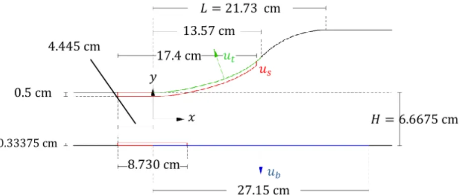
Figure 7: 2D profile of the diffuser examined in this work. The location of suction on the upper surface of the diffuser is shown in green and suction on the lower surface is shown in blue. Corner suction is shown in red.

A number of different suction patch configurations were tried with the final configuration shown in Figure 6 along with dimensions in Figure 7. The upper normal velocity is typically set at while the lower normal velocity is typically set at . The corner suction patches are also visible in the figures above. While the experiment uses small choked holes to maintain a particular mass flow, the CFD simply applies a normal velocity over the entire corner suction patch. In most simulations, is set to to match the mass flow that the experiment’s original suction pump can achieve. Some simulations increase this by and result in a nearly symmetric separation pattern when .

2.3

Mesh Generation

All meshes used for results are boundary layer meshes generated with BLMesher, a SCOREC (Scientific Computation Research Center) tool built upon the Simmetrix mesh generation APIs. The boundary layer meshes contain stacks of thin, highly anisotropic elements placed over no slip walls to resolve the boundary layer velocity gradients that arise from viscous Navier Stokes. The thickness of the first BL element, , nominally places the first node off of the wall at a nondimensional wall distance of roughly . The thickness of each subsequent layer,

, grows geometrically with a ratio such that and the total thickness of the boundary layer stack is

∑

(8)

The number of layers, , and the geometric growth ratio are typically set so that the boundary layer mesh fully encloses the velocity boundary layer. The main exception to this occurs when the surface mesh on a wall is small when compared to the thickness of outer layer BL elements. In this case, the outer elements are removed to preserve

𝑢𝑠 𝑢𝑡 𝑢𝑏 𝐿 𝑦 𝑥 _𝐻

a minimum aspect ratio between in-plane element length and thickness. This prevents the formation of “tall” elements. With meshes not intended for adaptation, this trimming occurs when element aspect ratios drop below 1. When adaptation is planned, this threshold is increased to 4. In all simulations, the wedges which initially make up the boundary layer are tetrahedronized for load balancing.

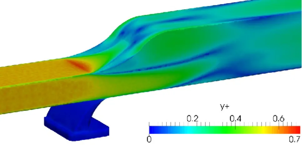
Figure 8: of the First Node Off of the Wall. The picture is taken from a time averaged Series 12 simulation with no flow control activated. The first element height is uniformly _{. For this setup, ( ) .}

In most meshes, the height of the first node off of the wall is kept constant at _{. With series 12 and 14,} the first layer thickness decreases to _{in the main flow path and in the blowers. In all cases, a}

posteriori examination of the flow field (such as in Figure 8) indicates that the first nodes off the wall are situated at a of at most ( ). A moderate geometric growth ratio of between and is used consistently in all boundary layers of a mesh. Coupled with to layers in the main flow path, the total thickness varies between and and the viscous sublayer, buffer layer, and log-law region are well resolved. Fewer layers are used in the blowers, primarily because of interference issues with the boundary layer on the opposite wall. Near very fine features such as the blower fillets, as few as 12 layers are used; the flow there quickly becomes three dimensional with large gradients perpendicular to the BL stack. In such situations, isotropic interior elements are better suited.

Outside of boundary layers in the mesh interior, isotropic elements are used. Especially in the diffuser, the isotropy of the elements allows turbulent eddies to be properly resolved in DDES and for complicated 3D structures to emerge with RANS. To conserve elements, refinement boxes are used to only resolve regions of interest. Most meshes use a ( ) long refinement region that captures the throat, the diffuser, and the region immediately downstream of the diffuser with elements. Neglecting boundary layers, this spacing results in approximately

38 elements across the width of the duct which is slightly more than the bare minimum of 32 elements suggested by Spalart to resolve a focus region for DDES [10]_{. Regions where separation is expected to occur are further refined}

with elements as shown in Figure 9 resulting in a fairly good initial mesh for both DDES and RANS.

\

Figure 9: Various mesh refinements used with upper and lower blowers.

Even smaller elements refine the flow control features. The corner suction patches use surface mesh lengths which propagate through the boundary layer stacks while the blowers use a series of progressively finer refinement boxes. Both blowers are surrounded by elements while the shear layer near the lip is captured by

_{elements. The separation zones immediately adjacent to the blower lips are resolved with elements and the blower lips themselves use a surface mesh. See Figure 9} for visual clarifications. Some variation exists between mesh versions, but this is fairly representative of most initial

elements elements elements elements elements elements elements elements

meshes. When blowers are present, additional refinement through adaptation is necessary to more judiciously add element and resolve the finer features of the flow.

At the other extreme away from the diffuser, the mesh progressively coarsens to , , and eventually

elements. This is done not only to save elements, but to get around acoustic issues. PHASTA presently cannot apply non-reflecting boundary conditions. As a result (according to Prof. Jansen [11]), when the contraction section is shortened or removed, waves generated in the test section reflect back into the test section and can become quite substantial. The coarse elements near the inlet and outlet provide numeric dissipation to attenuate these waves.

The mesh sizes used in different series vary dramatically. The clean, no blower numerical geometries typically used 15M to 20M elements (where M stands for million) and 2.5M to 3.3M nodes. This includes the contraction section, throat, diffuser refinements, and outlet. Including the lower blower adds an additional 20M elements. Unfortunately, the version of BLmesher used for mesh generation does not have a good way to specify anisotropic surface or interior elements. Consequently, the same resolution required to resolve the blower fillet curvature is also applied along the length of the fillet. This is enormously expensive and doubles the mesh sizes of series 12 to about 43M elements and 7.5M nodes. However, this is consistent with the single jet initial meshes used by Chen [3]_{. In}

series 14, the refinement boxes used to resolve the shear layer also splits the boundary layer stack. This again doubles the mesh to around 87M elements.

Chapter 3

Diffuser Design

Near the beginning of the project, the sponsor provided several diffuser geometries designed to create nearly constant pressure gradients ranging from ( ) to ( ). Because early simulations showed that the lowest pressure gradient diffuser was already massively separated, the research team collectively decided to focus attention on that design.

3.1

Pressure Gradient Design

The geometry targets a constant pressure gradient over roughly the first of the diffuser length. For initial design purposes, the flow was assumed to behave in a quasi-1D manner, even though the upper surface deviates by as much as 6_{. With this assumption, Shapiro’s influence coefficients give the relation} [12]

(9)

where the Mach number is governed by the separate ODE

( ) ( ) (10)

This creates a system of ODEs that can be numerically solved to obtain ( ). Alternatively, because ( ) is known,

( ) can be calculated from eq. (6) with ( ) taking the place of . From there, the area Mach number relation yields ( ). Both methods give the same results and are used, more or less, interchangeably.

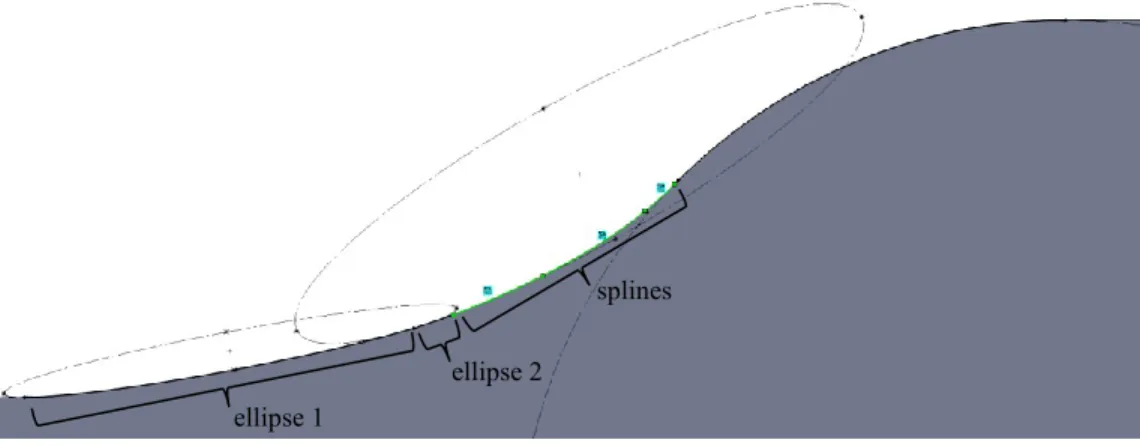
The geometry provided by the sponsor did not perfectly match the shape dictated by the quasi-1D flow equations. Instead, it approximated the constant pressure gradient diffuser with a series of ellipses and splines as shown in Figure 10. Moderate deviations are present near the inlet where the upstream throat ceiling smoothly transitions to the first ellipse. Downstream of the constant pressure gradient section, an arc smoothly transitions to the horizontal ceiling. At all junctions, continuity is enforced to try to minimize pressure spikes.

6 _{At least with respect to pressure and temperature, the quasi-1D assumption is surprisingly good. Near the bottom of the duct, the}

closest point on the ceiling is slightly upstream and closer than the point directly overhead. Consequently, the flow “sees” a slightly smaller area along with the lower pressures and temperatures associated with a higher Mach number. Towards the top of the duct, the effective area is slightly larger for similar reasons, but the flow is heavily influence by the local ceiling curvature. The curvature dominates and happens to drop the pressure and temperature to similar values observed on the floor.

Figure 10: Construction of Provided Geometry. The first 41% of the diffuser is approximated by two ellipses (solid black), followed by a set of splines (light green) and then an arc to maintain continuity at the AIP.

It is unclear why this combination of geometric primitives was chosen over doing the entire surface with a spline. Referring to Figure 12, deviations from the nominal pressure gradient exceed 10% near the middle of the diffuser. Upstream, the continuity with the throat ceiling also forces to drop to zero. However as discussed in section 3.3, the high curvature in this region still dominates the effects from area change and produces a very large low pressure spike.

Figure 11: Geometry Shape and Upper Surface Slope of

Series 1. Figure 12: Expected Quasi-1D Pressure distribution of Series 1. The targeted pressure gradient is shown in red.

-0.1 0 0.1 0.2 0.3 -0.05 0 0.05 0.1 0.15 x (m) y (m ) -0.1 0 0.1 0.2 0.3 -2 0 2 x (m) dy/ dx -0.16 0 0.1 0.2 0.3 8 10x 10 4 p (P a) -0.10 0 0.1 0.2 0.3 1 2x 10 5 x (m) dp/ dx (P a/ m ) ellipse 1 ellipse 2 splines

3.2

Selection of Suction Velocities

As already mentioned, the geometry produces substantial separation off of the upper surface. This drops the effective area change and, consequently, the static pressure gradient. To analyze the eventual pressure gradient of the diffuser with effective flow control, suction patches are added to the floor, ceiling, and corners as shown in Figure 6. The corner patch mass flows are constrained by the experimental suction pump to have a maximum normal velocity of about . However, the selection of the upper and lower suction patch velocities is not

immediately obvious; the magnitudes need to be iterated until acceptable performance is observed. To save resources and allow for faster iteration, URANS is used instead of DDES7. This allows reasonable statistics to be collected over a few thousand time steps instead of tens of thousands.

There are few good quantitative metrics to use for numeric optimization. The distortion at the AIP is one of the better options, but when measured with a scalar distortion metric such as a rectangular version of ( ) found in reference [13], it loses information about where the separation actually occurs. Trying to minimize the linear terms of a 2D polynomial expansion of is an interesting option that retains information about where separation occurs, but was proposed after the fact. There is also the question of how to deal with unsteadiness; even in locations where the mean flow is attached, substantial unsteady backflow may be present over short intervals of time. Because of the ambiguity over how to synthesize these metrics, any cost function for numeric optimization would be almost as subjective as simply looking at the flow field (as well as substantially more work). For this reason, the iteration was conducted manually. The flow was visualized with several different filters including -normal and -normal slices, velocity contours, and continuous time data sampled at discrete points in the fluid domain. In general, separation on the top of the duct required to be increased while separation on the bottom required to increase. The

velocity contours tend to give a good idea of this process.

7 _{Inviscid Euler simulations are a potentially viable alternative for diffuser design. An inviscid simulation would inherently}

prevent separation and, consequently, get rid of the need to use suction patches. However, some features of the duct (such as the corner suction) are specifically designed to counter viscous phenomena.

Figure 13: Velocity Contour of Instantaneous Flow field with and .

Figure 14: Velocity Contour of Instantaneous Flow field with and .

Using only the upper suction patch with a velocity of and full corner suction with , the flow is still reminiscent of the baseline flow in section 4.1 that develops without any suction. The momentum in the upper surface boundary layer is insufficient to navigate the adverse pressure gradient, and high velocity backflow in one corner of the duct intrudes past the end of the suction patch. Increasing the mass flow through the ceiling patch by only 33% produces a profound effect on the flow with most of the inviscid core lifting up off the floor and one of the side walls as shown in Figure 14.

Figure 15: Velocity Contour of Instantaneous Flow field with and .

Figure 16: Velocity Contour of Instantaneous Flow field with and .

Separation on the floor is dealt with by thinning the boundary layer with the bottom suction patch. However, attaching the floor increases the pressure gradient and shifts the separation back to the upper surface. Consequently, both suction velocities need to be increased. With and , minor improvements are observed with a more symmetric and slightly smaller floor separation. Increasing to , large sustained

separation structures on the floor largely disappear leaving intermittent pockets of backflow. However, by this point, the large pressure gradients fighting against the high momentum boundary layers make the separation patterns very unstable and intermittent. It is consequently more instructive to switch to time averaged fields.

Figure 17: Velocity Contour of Time Averaged Flow over with and .

Figure 18: Velocity Contour of Time Averaged Flow over with and .

As both and increase further, the benefits begin to diminish. Comparing the time averaged contours in Figure 17 with Figure 18, only minor differences are visible, despite a roughly 20% increase in mass flow through the suction patches. Increasing to results in a moderate reduction of the unsteady RMS velocity8 _{on the floor,}

but this comes at the cost of slightly increasing the strength of separation on the walls. Further increases are possible, but even at the / patch velocities, over of the primary flow is being removed as indicated in Table 2. Due to concerns about unduly influencing the flow physics, the lowest reasonable values of

and are used in section 3.3 to iterate the diffuser shape9_.

Table 2: Effective Areas and Mass Flow Rates with and

Patch Normal Velocity Area (effective) ̇ ̇ fraction

Top Bottom Upper Side Lower Side Cumulative Side

8 _{That is, (} ̅̅̅̅) _{where ̅ and} ̅ _{denotes an average over time.}

3.3

Iteration of Initial Diffuser Curvature

The pressure gradient of the series 1 diffuser (shown in Figure 19) deviates substantially from the targeted gradient. Near , a spike in local curvature produces a large increase in velocity which is accompanied by a severe drop in the pressure. This effect dominates the pressure gradient for about on either side. Downstream at about , the diffuser again sees over a jump in curvature. This sets up a similar drop in pressure below what is predicted by the quasi-1D equations with diminished upstream of the jump and inflated downstream of the jump.

Also note that the flow becomes fairly three dimensional after about . There is a higher speed core of fluid in the center of the duct that is fairly sensitive to the larger curvatures near the diffuser profile inflection point. On either side, the average pressure recovery drops to about half of the target gradient. Both intermittent separation on the side walls and deviations from the 1D flow assumptions are likely contributing factors, but it is still unclear how significant these mechanisms are and without flow control on the side walls, it is difficult to separate the two effects.

Figure 19: Ramp curvature and CFD pressure distribution on the original geometry. Yellow curvature combs are shown with the geometry to the left.

There are several options for improving the pressure gradient. A fairly promising methods involves estimation of curvature effects from the linearized potential equation below.

( )

(11)

In equation (11), is the velocity perturbation from the freestream and is the velocity potential. With a

rectangular domain ( ) ( ) where , a parabolic velocity profile is applied to the upper edge. is varied to generate a response map of pressure drop as a function of curvature. This map is then

-0.2 -0.1 0 0.1 0.2 0.3 0.4 0.5 80 100 p (x ) (k P a) -0.2 -0.1 0 0.1 0.2 0.3 0.4 0.5 -200 0 200 axial position (m) d p /d x (P a/ m m ) z = -0.25D z = 0 D z = 0.25 D

used to filter the quasi-1D profile. However, manual iteration of the diffuser geometry yielded “adequate” results before a diffuser could be designed from perturbation theory.

Figure 20: Ramp curvature and CFD pressure distribution on an intermediate geometry after some iteration. The altered curvature of the new geometry is shown with green curvature combs.

In series 5 (Figure 20), the original ellipse at the beginning of the duct is replaced by one with lower eccentricity. This more evenly distributes the curvature and gets rid of the overshoot near . Moderate overshoot is present in the viscous simulation and the quasi-1D profile, but it is substantially less pronounced. The second curvature discontinuity is still present and results in a similar dip in at as is seen in series 1.

Figure 21: Expected quasi-1D pressure distribution of

Series 5. The targeted pressure gradient is shown in red. Figure 22: Expected quasi-1D pressure distribution of Series 8. The targeted pressure gradient is shown in red. In series 8 (Figure 22 and Figure 23), both ellipses shown in Figure 10 are replaced by a single, large ellipse. The curvature near the beginning of the diffuser increases slightly and pulls the location of the maximum pressure gradient forward, but it has little effect on the magnitude. In the middle of the diffuser, the more uniform curvature is seen as a less severe jump in . The gradient still falls off substantially towards the end of the diffuser, but making the differ more aggressive in this region without adding side wall suction would likely induce further separation. -0.2 -0.1 0 0.1 0.2 0.3 0.4 0.5 80 100 p (x ) (k P a) -0.2 -0.1 0 0.1 0.2 0.3 0.4 0.5 -200 0 200 axial position (m) d p /d x (P a/ m m ) p, z = -0.25D p, z = 0 D p, z = 0.25D -0.16 0 0.1 0.2 0.3 8 10x 10 4 p (P a) -0.10 0 0.1 0.2 0.3 1 2x 10 5 x (m) dp/ dx (P a/ m ) -0.16 0 0.1 0.2 0.3 8 10x 10 4 p (P a) -0.10 0 0.1 0.2 0.3 1 2x 10 5 x (m) dp/ dx (P a/ m )

Figure 23: Ramp curvature and CFD pressure distribution on the geometry which was sent for manufacturing. The altered curvature of the new geometry is shown with green curvature combs.

It is also important to remember that suction patches are only surrogates. They are altering the flow path and creating extra effective curvature in ways that tangential blowing does not. Additionally, the gradual drop in

likely suits tangential blowing; the adverse pressure gradient is decreasing at the same time that the strength of the jet is decreasing. For these reasons, along with wanting to move on, the series 8 diffuser geometry is used in the experiment and all subsequent geometries.

-0.2 -0.1 0 0.1 0.2 0.3 0.4 0.5 80 100 p (x ) (k P a) -0.2 -0.1 0 0.1 0.2 0.3 0.4 0.5 -200 0 200 axial position (m) d p /d x (P a/ m m ) z = -0.25D z = 0 D z = 0.25D

Chapter 4

Separation Dynamics and Flow Control

4.1

No Blower Results

The series 8 geometry was run with URANS in a number of configurations including a true baseline with no active flow control, a corner suction baseline with only side wall suction, and a full suction case where the ceiling and floor suction normal velocities are set respectively to and in addition to the corner suction. With the true baseline and the corner suction baseline, DDES runs were also performed to provide a more accurate comparison with experiment. However, the differences between CFD and experiment are not fully understood at this time and will not be presented. DDES simulations of the full suction case do not have an experimental equivalent and were not run.

4.1.1 URANS and DDES with No Suction

As already mentioned, the additional momentum deficit in the corners of the duct predisposes the flow to separate there as the adverse pressure gradient increases. This is evidenced by the V shaped pattern in Figure 24 with backflow extending almost to the start of the diffuser. However, the downstream sidewall separation is clearly asymmetric in this configuration. Inevitably, numeric or physical perturbations result in one of the corner pockets growing slightly larger than the other. This translates to higher upstream pressures that accelerate the flow towards the other wall. The extra momentum directed at the smaller separation pocket further shrinks it while increasing the effective area of the diffuser and the adverse pressure gradient. In turn, this feeds the larger separation pocket.

Figure 24: Streamlines and Velocity Contour of

Baseline URANS Time Averaged Flow over . Figure 25: Streamlines and Baseline DDES Time Averaged Flow over Velocity Contour of .

The backflow substantially reduces the effective area and drops the pressure gradient enough for the flow to remain mostly attached on one side. There, it picks up a moderate amount of vertical momentum. This momentum is carried with the fluid past the AIP and sets up a strong downstream swirl. As fluid near the ceiling of the duct in Figure 24 moves to the far wall, it is replaced by fluid originating from the floor. At the same time, the cross sectional area of the duct continues to increase resulting in a sustained, albeit less severe, adverse pressure gradient. These two effect combine to extend the side wall separation onto a large portion of the floor.

Figure 26: Series 8 URANS No Suction Mach Contours. Results are averaged over 2400 time steps corresponding to an interval of . Dark isolines are drawn at increments.

Both the URANS and DDES flow fields have the same qualitative asymmetry, but some differences are present. Referring back to Figure 25, the primary DDES separation contour is slightly smaller and obviously does not reach the floor. This is also seen when comparing the Mach slices in Figure 26 and Figure 27 taken at and (where is the full with of the duct). The DDES turbulence model predicts higher diffusion of momentum

which tends to shorten almost all the features of the flow. The effect is most pronounced on the slices where the larger, lower frequency structures lead to noisier statistics after .

Figure 27: Series 8 DDES No Suction Mach Contours. Results are averaged over 20000 time steps corresponding to an interval of . Isolines are drawn at increments.

Both the URANS and DDES separation contours are fairly stable. While it is entirely possible that the

separation will switch sides given enough time, such switching in a baseline configuration has yet to be observed in any simulations. It appears that the asymmetric swirl corresponds to a rather low energy state of the flow; once the flow picks a side, it takes a substantial disturbance to escape to the reflected state.

4.1.2 RANS and DDES with Corner Suction

As corner suction is increased, the local boundary layer is thinned and the corner momentum deficit drops. This delays the onset of separation and reduces the adverse stress seen by fluid farther away from the wall. Ideally, the viscous sidewall effects are completely hidden from the ceiling boundary layer resulting in quasi-2D separation as intended by the experiment.

According to simulations, the corner suction velocity that the experiment can achieve is not sufficient by itself to fully symmetrize the flow. Both RANS and DDES results indicate that moderate downstream vorticity is still generated in a similar manner as the baseline case. However, the sidewall boundary layers have enough momentum to stay attached and keep the ceiling vortex concentrated in the upper half of the duct. The separation contour in Figure 28 is also somewhat deceptive; a shear layer extends across the entire duct. The right side of the duct contains strong ( ( ) ) backflow while the left side acts as a low speed return path.

Figure 28: : Streamlines and

Contour of URANS with

Corner Suction averaged over .

Figure 29: Streamlines and

Contour of URANS with

Corner Suction averaged over .

Figure 30: Velocity contour of DDES with Corner Suction Averaged over

As corner suction increases further to , URANS predicts very little changed to the overall flow field; Figure 28 looks almost identical to Figure 29. However, the behavior of the DDES simulation changes dramatically; by , the separation pocket is largely two-dimensional.

pre ss ure Ed dy Visc osity

Figure 31: Series 8 DDES Corner Suction Mach, Pressure, and Eddy Viscosity at the Centerline. Results are averaged over 20000 time steps corresponding to an interval of . Dark isolines are drawn at intervals of and .

The pressure, eddy viscosity, and Mach fields at the centerline of the DDES simulation in Figure 31 are representative of the states across most of the duct; other slices are unnecessary. For comparison, slices of the URANS flow field in Figure 32 have been made at the same location. The differing behavior of the flow is evident in the pressure field; DDES shows no discernable pressure change near the ceiling in the second half of the ramp while the RANS simulation has to contend with reversing a jet of fluid. Similarly, as expected, DDES generates very little eddy viscosity in the upper half of the ramp, instead resolving a large portion of the Reynolds stresses of the relatively slow flow there. URANS has a to model the turbulent stresses of a fairly strong shear layer running over half a meter back with high EV production.

pre ss ure Ed dy Visc osity

Figure 32: Series 8 URANS Corner Suction Mach, Pressure, and Eddy Viscosity at the Centerline. Results are averaged over 2000 time steps corresponding to an interval of . Dark isolines are drawn at intervals of and .

These differences highlight the difficulty of dealing with massively detached flow; turbulence models begin to break down and give substantially different results. In general, DDES tends to do better in situations like this, but it does not constitute reality; experimental validation is needed. Unfortunately, experimental results with corner suction are not yet available for comparison.

4.1.3 RANS with Full Surrogate Flow Control

The mean flow field separation contours of series 8 with full suction (i.e. , , and

) are very similar to those of series 1 seen in Figure 17. Backflow is present over large portions of both side walls in the diffuser, but a majority of the floor and ceiling remain attached as seen in Figure 33. The

concentration of high speed flow in the center of the duct means that there is an imbalance in vertical momentum at the AIP. However, instead of obtaining one large vortical structure as in the baseline case, two counter rotating primary vortices develop on either corner of the ceiling. This is clearly seen in Figure 34 where velocity vectors are projected onto a plane located a half diffuser length behind the AIP. Further downstream, the downward moving fluid on the sidewalls penetrates the floor boundary layer and lifts up the streamlines up as seen in Figure 33.

Figure 33: Streamlines and Velocity Contour of Full Suction URANS Time Averaged Flow over .

Figure 34: Velocity projected onto the plane.

While most of the floor does not separate in the sense of having negative mean velocity, the simulation does have a large, low speed pocket located at and behind the AIP. This pocket is not as substantial as the side wall separation, but should still contribute to the pressure gradient deficit observed in Figure 23. In this respect, it is clear that a higher bottom suction is needed if the floor boundary layer if to remain thin.

Figure 35: Series 8 URANS Full Suction Mach Contours. Results are averaged over . Dark isolines are drawn at

increments.

The mean velocity does not give a complete picture of what is happening. While back flow is present in both upper corners of the diffuser, the separation in one corner is usually more substantial than the other; the resulting unsteady contours are often reminiscent to the no suction URANS contours in Figure 24 and commonly extend past the centerline on the floor. However, the boundary layer thinning from suction prevents the separated region from growing to the same size and strength as the backflow in the baseline case. The high speed flow near the ceiling also never deviates enough from center to generate a particularly strong downstream vortical structure. The

net result is that unsteady fluctuations frequently cause the dominant side to switch. As the inviscid core in the duct shifts, very large RMS velocity fluctuations are observed at the AIP (Figure 37) and downstream. The unsteadiness near the floor is also reflected by the very high mean eddy viscosity that develops there (Figure 36). Indeed, ̃

downstream of the AIP becomes roughly 2 orders of magnitude larger than the eddy viscosity found in the turbulent boundary layer at the start of the diffuser inlet.

Figure 36: Series 8 URANS Full Suction Eddy Viscosity. The slice is taken at the , i.e. 4the centerline.

Figure 37: Series 8 URANS RMS Streamwise Velocity fluctuations at the AIP. Results are averaged over .

4.2

Coandă

Blowing

Like with series 8, the series 12 geometry (with a single blower on the floor) was run with several different flow control parameters. Configurations include a true baseline with no flow control, a symmetrized separation with

corner suction and a floor blower throat Mach number of , and full flow control with

ceiling suction and corner suction in addition to the blower. Simulations have also been run with tangential blowing on the ceiling (series 14), but those results are still preliminary; grid independence has yet to been established and the dynamics have not been examined. Consequently, only series 12 will be discussed in this section.

The symmetrized separation case is not particularly interesting; with only a 1% mass flow addition at the floor, the results are very similar to those shown in section 4.1.2. Flow control is not needed for already attached flow. However, when ceiling suction is added, the importance of the floor blower becomes clearly visible. With just ceiling and corner suction, the flow abruptly detaches from the floor before the midpoint of the diffuser (Figure 38). With the extra momentum from floor blowing, the detachment is delayed until after the AIP.