Differential-Private Data Publishing Through
Component Analysis
Xiaoqian Jiang
∗, Zhanglong Ji
∗∗, Shuang Wang
∗, Noman Mohammed
∗∗,
Samuel Cheng
∗∗∗, Lucila Ohno-Machado
∗∗Division of Biomedical Informatics, UC San Diego, La Jolla, CA 92093
∗∗Department of Computer Science, Concordia University, 1455 De Maisonneuve Blvd. W., QA H3G 1M8 ∗∗∗University of Oklahoma, 4502 E., 41st St #4403, Tulsa, OK 74135-2512
E-mail:[email protected]
Abstract. A reasonable compromise of privacy and utility exists at an “appropriate” resolution of the data. We proposed novel mechanisms to achieve privacy preserving data publishing (PPDP) satisfyingε-differential privacywith improved utility throughcomponent analysis. The mechanisms studied in this article are Princi-pal Component Analysis (PCA) and Linear Discriminant Analysis (LDA). The differential PCA-based PPDP serves as a general-purpose data dissemination tool that guarantees better utility (i.e., smaller error) compared to Laplacian and Exponential mechanisms using the same “privacy budget”. Our second mechanism, the differen-tial LDA-based PPDP, favors data dissemination for classification purposes. Both mechanisms were compared with state-of-the-art methods to show performance differences.
Keywords. differential privacy, data publishing, principal component analysis, linear discriminant analysis
1
Introduction
Dissemination and meaningful use of patient data can help improve treatment satisfaction, quality of life, and various aspects of well-being [1]. However, privacy is a major concern when patient data is used for research purposes [2]. Healthcare data often contain sensitive information about indi-viduals, and publishing such data might violate their privacy. Ensuring privacy while maintaining data utility is one of the most important problems in biomedical research [3, 4]. Loss of privacy is usually associated with failure to control access to information, to control the flow of information, or to control the purposes for which information is employed [5]. To provide strong privacy guarantees and to give researchers greater flexibility in conducting the required data analysis, it is necessary to develop utility-aware privacy preserving data publishing mechanisms. In this paper, we proposed two new privacy-preserving publishing algorithms that can effectively preserve data utility for vari-ous data workloads and achievesdifferential privacy, a rigorous definition that provides a provable privacy guarantee.
1.1
Motivation and Related Work
Data privacy has been an active research topic in statistics, database, and security community for the last three decades [6–9]. Many privacy models, such ask-anonymity [10] and its extensions [11, 12]
have been proposed to thwart privacy threats caused by identity and attribute linkages in relational databases. The usual approach is to generalize the records into equivalence groups so that each group contains at leastkrecords with respect to some quasi-identifier (QID) attributes, and the sensitive values in eachQIDgroup are diversified enough to prevent confident inferences. A large number of anonymization algorithms [13, 14], tailored for both general and specific data mining tasks, have been proposed based on these privacy models.
However, Wong et al. [15] showed that these algorithms are vulnerable to minimality attack and do not provide the privacy guarantees. Subsequently, more privacy attacks such ascomposition
attack[16],deFinetti attack[17], andforeground knowledge attack[18] have emerged against these
algorithms [13, 14].
Differential privacyhas received considerable attention recently as a substitute for aforementioned
partition-based models for privacy preserving data publishing (PPDP). A differentially-private mech-anism ensures that the probability of any output (released data) is equally likely from all nearly identical input data sets and therefore guarantees that all outputs are insensitive to an individual’s data. Most of the research on differential privacy concentrates on non-data publishing with the goal to reducing the magnitude of added noise [19, 20], or releasing certain data mining results [21, 22]. These techniques completely prohibit the sharing of data. When compared to sharing the results of data mining, data sharing gives greater flexibility because recipients can perform their required analyses and data exploration, and apply different modeling methods and parameters.
Current techniques that allow data sharing publish contingency tables of the original data [20, 23–25]. These techniques generally add Laplacian noise to the raw counts of records to ensure differential privacy. The Laplacian mechanism has two main limitations. First, Laplacian noise on counts could eliminate almost half of the small counts, since negative counts are considered as zero. Second, Laplacian noise is unbounded, which could result in released data to be unexpectedly large, and with a few records sampled repeatedly, dominating the entire database. Thus, these techniques may significantly destroy the data utility. We also confirmed this point by experiments in Section 4.
1.2
Contributions
In this paper, we propose two privacy-preserving data publishing (PPDP) mechanisms: differential PCA and differential LDA. The proposed mechanisms build a compact, privacy-preserving synopsis based on component analysis with a fixed amount of privacy budget. Synthetic data are generated from the privacy-preserving synopsis to answer any queries or build data mining algorithms without decreasing the level of privacy protection. Ourcomponent analysisbased privacy preserving data publishing (PPDP) mechanisms add noise, mostly on the first and second moments (i.e., mean and variance-covariance) rather than on the original data or their contingency tables. This reduces the required amount of noise and enables us to provide the same privacy protection with less perturba-tion compared to existing techniques. Next, we briefly present the key advantages of the proposed mechanisms.
1. The differential PCA-based PPDP generates synthetic data with aone-to-onemapping to the original data, and preserves the order information. This is essential for data custodians to pub-lish time-series data (i.e., lab tests) or enable privacy preserving sequential release of attributes from the same database.
2. The differential LDA-based PPDP provides great flexibility in generating synthetic data, which provides a better preservation of the original data distribution. Experimental results demon-strated that the proposed LDA-based PPDP outperforms the recently proposed differentially-private data release algorithm [25] for different utility metrics.
A similar mechanism to our PCA-based PPDP called SuLQ [26], which is also based on principle component analysis, however, is different from our work in its purpose (i.e., query in the projected subspace vs. data publishing) and noise addition procedures (i.e., adding Gaussian noise to variance-covariance matrix in SulQ vs. adding Laplacian noise to both variance-convariance matrix and projected data in our case). We are not aware of similar works to our LDA-based PPDP.
The rest of the paper is organized as follows. Section 2 reviews Principle Component Analysis (PCA), Linear Discriminate Analysis (LDA), and Differential Privacy (DP). Our component-analysis based privacy preserving data publishing mechanisms are explained in Section 3. Section 4 exper-imentally evaluates the performance of our methods and compares to the state-of-the-art models. Section 5 concludes the paper.
2
Preliminaries
Principle Component Analysis (PCA)is an analysis method that converts observations of random vectors into orthogonal principal components, while the number of principal components can be either equal or smaller than the dimension of the original data. When the number of components is smaller than the dimension of the original data, we can project the original data to the space of these principal components to get a low-rank approximation. The idea behind this approximation is to preserve as much information of the original data (i.e., the criterion is to minimize the F-norm of the approximation error) as possible. Mathematically, given a matrixXn×prepresenting then-record
and p-dimensional data, PCA decomposes the variance-covariance matrixD=Var[X] =UTVU, whereUis an orthogonal matrix consists of eigenvectors, and
V=diag{λ1,λ2, . . . ,λp},
λ1≥λ2≥ · · · ≥λp≥0
are the eigenvalues. The eigenvectors are also called principal components. SupposeUkis the firstk
eigenvectors ofVar[X], we can get an approximation ofXby computing (X−E[X])UkTUk+E[X].
Based on linear algebra, we know that
(X−E[X])UkTUk+E[X]−X 2 F= λk+1+· · ·+λp λ1+· · ·+λp kX−E[X]k2F.
For correlated data, the ratio between meaningful eigenvectors and total eigenvectors is usually small, i.e., there exists somekp,λk+1+···+λp
λ1+···+λp '0.
Linear Discriminant Analysis (LDA)is a classification algorithm based on component analysis. It assumes that data in each class comes from a Gaussian distribution, and it uses the probability density to classify new samples. For example, suppose the data in classCihave a mean ofµiand a
variance-covariance matrixΣ, then for each new datax, the probability
P(x∈Ci)∝exp(−1 2log|Σ| − 1 2(x−µi) T Σ−1(x−µi)).
To predict the class to which the sample belongs, we just need to compare the probabilities. Differential privacy (DP)is a cryptographically motivated privacy criterion proposed by Dwork [27], which assumes that any results (i.e., through query operations) of a “private” data set should not drastically change with an addition, deletion, or update of a single record. The Laplacian mechanism is a common way for achieving differential privacy.
Definition 1(ε-Differential Privacy). A randomized algorithm (or mechanism)Agis differentially private if for all data setsDandD0, where their symmetric difference contains at most one record, and for all possible anonymized data sets ˆD,
Pr[Ag(D) =Dˆ]≤eε×Pr[Ag(D0) =Dˆ], (1) where the probabilities are over the randomness of the algorithmAg.
Theorem 1[20] (Laplacian mechanism) For any function f :D→R, the algorithmAgthat adds noise with distributionLap(s/ε)(wheres=maxD,D0k(f(D)−f(D0))k1denotessensitivityandε stands for theprivacy budget) to the outputs of f(·)satisfies differential privacy.
3
Methodology
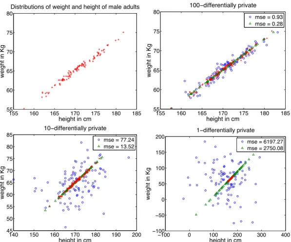
We first illustrate our intuition why component analysis could help. In the simplified example showed in Figure 1, we considered a data set of 100 male adults with two highly correlated attributes: height and weight. Here, we considered theidentity queryas in [28]. It publishes the data matrix directly instead of some other queries (e.g., count query) that preserves the property of the data set. To ensure privacy for identity query, one should intuitively perturb each data point. Note that since each record can be considered as a disjoint data set, parallel composition [29] holds, and thus we can ensure the entire data set to beε-differentially private as long as each record isε-differentially private. However, the height and weight queries do not apply to disjoint sets of record. Therefore, based on sequential composition [29] , we evenly split theεbudget separately into the two attributes for ensuring each of them to beε/2-differentially private1. On the other hand, if the appropriate “component” is picked (i.e., using common knowledge about weight and height), we do not need to split the budget but can use the entireεfor a single dimension. As a result, the mean squared error (MSE) can be significantly reduced. More importantly, as illustrated in the figure, the statistics of the data change drastically if we naively apply noise to each dimension (attribute) independently. This could make the data virtually unusable. In reality, the common knowledge about components does not always exist. Therefore, it is necessary to use component analysis to find the major components so that noise is added to fewer but most important “parts” of data without decreasing the level of privacy protection. In this paper, all the expectations mean empirical expectation. A replace of sam-ple will not change the expectations on the underlying distribution, but it does change the empirical expectation.
3.1
Differential PCA
In differentially PCA, we add noise in both projection and recovery steps as mentioned in Section 2. First, we decompose anoisy variance matrixinstead of the exact matrix. Second, we add noise to
theprojected matrixbefore recovery. Suppose the samples arep-dimensional i.i.d. random vectors
X1,X2, ...,Xn, this mechanism guarantees better better performance than the Laplacian mechanism
(i.e., on the raw data) in terms of F-norm, ifnεp2andε2+k2≤p2(the latter is often true since we usually havek<pand smallε).
Both conditions will be justified in Theorem 3 but let us first discuss how to get differentially private
E[X]and upper triangleEX XTfromX, which are essential to this mechanism. Specifically, we only consider the upper triangle ofEX XTbecause of its symmetry, i.e., if we change its upper triangle, we can just copy the noisy entries to the lower triangle.
1The optimal solution might correspond to an uneven split of the budget. We did not intend to study the optimal budget allocation for this illustration example.
155 160 165 170 175 180 185 55 60 65 70 75 80 height in cm weight in Kg
Distributions of weight and height of male adults
155 160 165 170 175 180 185 55 60 65 70 75 80 height in cm weight in Kg 100−differentially private mse = 0.93 mse = 0.28 140 150 160 170 180 190 200 45 50 55 60 65 70 75 80 85 height in cm weight in Kg 10−differentially private mse = 77.24 mse = 13.52 −100 0 100 200 300 400 −100 −50 0 50 100 150 200 height in cm weight in Kg 1−differentially private mse = 6197.27 mse = 2750.08
Figure 1: Two versions of noisy data after applying the Laplacian mechanism to: (1) a principal component (noisy results indicated by ‘4’), (2) the original domain (noisy results indicated by ‘o’), of simulated weight and height data of male adults (’+’). The difference of mean squared errors (MSE) between component aware and unaware approach increases as the privacy budget decreases. For example, for privacy budget,ε=1, the difference is (6197.27 - 2750.08) as shown in the lower-right figure. Our interested ranges for both weight and height were predetermined before getting the data, therefore, sensitivity is independent of the data.
Suppose each variable is clamped to[0,1], and there arepnumerical variables in total, the sensi-tivity of∑x∈Xxand upper triangle∑x∈XxxT ares=p+ (p+1)p/2. The detailed differential PCA
is as follows. (The mechanism for data set with categorical variables will be discussed later). PCA-based PPDP Mechanism:
1. Given a data set (or matrix) Xn×p. Suppose each entry in the set is bounded to [0,1], we
compute∑x∈Xxand∑x∈XxxT.
2. Get noisy sums ofxandxxT by addingLap(2s/ε)on each entry of∑x∈Xxand upper triangle
of∑x∈XxxT, then fill in the lower triangle of∑x∈XxxT with the upper triangle symmetrically.
3. GetE[X]noisyandEX XTnoisyby dividing the noisy sums by sample numbern. 4. Step 3 ensures that
D=EX XTnoisy−E[X]noisyE[X]Tnoisy
is a symmetric matrix. Thus, we can eigen-decompose itD=UTV U, and select thek≤p
eigenvectors that have the largest eigenvalues fromU to formUk.
5. Add noiseLap(2√k p/ε)on(X−E[X]noisy)UTk, multiply it byUk, and addE[X]noisyto each
sample to get noisyX. Proof of differential privacy:
Lemma 1E[X]noisyandEX XTnoisyareε/2-differentially private.
Proof. The sum of sensitivities of∑x∈Xxand∑x∈XxxT iss, thus the noisy sums in the second step
areε/2-differentially private, and so areE[X]noisyandEX XTnoisyin the third step. Lemma 2GivenUTk, the sensitivity of(X−E[X]noisy)UTk is√k p.
Proof. SinceXUTk is ann×kmatrix, and each sample only affects one row in it, we only need to
prove that for anyx1andx2there is
(x1−x2)U T k 1≤ p k p
Since there arekorthogonal components inUkwhich are all unit length vectors, we can useu1touk
to represent them. The maximum value of
(x1−x2)U T k 1is max∑ k i=1|(x1−x2)Tui|. Since k
∑
i=1 |(x1−x2)Tui| !2 ≤ k k∑
i=1 |(x1−x2)Tui|2 ≤ kkx1−x2k22 ≤ k p, the maximum value is therefore less than√k p.Proof. In step 5 of the PCA-based PPDP mechanism, we add noiseLap(2√k p/ε)to(X−E[X]noisy)UTk
(i.e., which has a sensitivity of√k p), therefore making itε/2-differentially private. Theorem 2The differential PCA mechanism isε-differentially private.
Proof. For any data setsD1andD2that differ at most one entry, we have (suppose the data matrix
inD1isX1and that inD2isX2) P XX1 P XX2 = R P X E[X]noisy,E X XTnoisy,XUTk(noisy) P
E[X]noisy,EX XTnoisy,XUTk(noisy)
X1 R P X E[X]noisy,E[X X T] noisy,XU T k(noisy) P E[X]noisy,E[X XT] noisy,XU T k(noisy) X2 ≤ max
E[X]noisy,E[X XT]noisy,XU T k(noisy) P
E[X]noisy,EX XTnoisy,XUTk(noisy)
X1 P E[X]noisy,E[X XT] noisy,XU T k(noisy) X2 ≤ max
E[X]noisy,E[X XT]noisy,XU T k(noisy) P XUTk(noisy) E[X]noisy,E X XTnoisy,X1 P E[X]noisy,EX XTnoisy X1 P XUTk(noisy) E[X]noisy,E[X X T] noisy,X2 P E[X]noisy,E[X XT] noisy X2 ≤expε 2 expε 2 =exp(ε).
Theorem 3Differential PCA based PPDP adds smaller noise compared to the Laplacian mechanism in terms of F-norm, given: (1)nεp2; (2)ε2+k2<p2.
Proof. The noise of this method comes three ways: approximation of p-dimension data with
pro-jection onk-dimensional space, the noise on the variance-covariance matrixD, and onXUTk. The first is λk+1+...+λn
λ1+...+λn kX−E[X]kF =
λk+1+...+λn
λ1+...+λn O(pn). The second part is very small whennεp 2 because the sensitivity is at mostO(p2/nε). Whennεp2, the difference betweenDandDare small, thus the approximation error is also small. The third part is the main source of noise. Its variance is aboutO(k2pn/ε2)(knentries, each added noiseLap √k p/εhas varianceO(k p/ε2)). The noise of the Laplacian mechanism isO(p3n/ε2)(pnnoise, eachLap(p/ε)). Thus, our method is better by F-norm when
λk+1+...+λn
λ1+...+λn
O(pn) +O(k2pn/ε2)≤O(p3n/ε2).
That is, if λk+1+...+λn
λ1+...+λn ≤1 is always true andε
2+k2<p2, our method adds smaller noise.
How to deal with categorical variablesAlthough PCA was developed for numerical variables, we can use them for categorical variables. Suppose there arep1numerical variables which have been normalized to[0,1], andp2categorical ones. We followed the common practice to change them into dummy variables, and treat these dummy variables as numerical variables in the PCA.
There are two differences introduced by categorical variables. First, the sensitivity is significant lower. Although one categorical variable may generate many dummy variables, only one of them can beonein a sample, and the others are all zeros. The largest change of∑x∈Xxand upper triangle
of∑x∈XxxT is achieved by changing all numerical variables from zero to one (or from one to zero),
and all categorical ones at the same time. In this case,p2(orp1+p2) values are changed from one to zero andp1+p2(orp2) are changed from zero to one. Thus∑x∈Xxchanges with(p1+2p2)in terms ofL1norm, and the upper triangle of∑x∈XxxTchanges with[(p1+p2)(p1+p2+1) +p2(p2+1)]/2.
Therefore, the sensitivitysof(∑x∈Xx,upper triangle of∑x∈XxxT)is(p1+2p2) + [(p1+p2)(p1+
p2+1) +p2(p2+1)]/2. Note that the number of different values of one variable does not contribute to the sensitivity.
The second difference comes from the value recovery. Since the noisy outputs are continuous, it is necessary to recover the categorical variables from dummy variables. In differential PCA, the recovery is simply picking the largest value of noisy outputs so that one category is selected. In this way, the output can keep the same format (i.e. categorical) as the input.
3.2
Differential LDA
This mechanism aims at preserving as much information as possible for classification algorithms instead of the original data, which makes it different from the first mechanism.
As the LDA only uses the means and variance-covariance matrices (here we assume that all classes have the same variance matrix to reduce sensitivity) of data in different classes, we must preserve as much information on them as we can. Our idea is first to get these noisy statistics, and then generate data from them. Suppose there are two classes (in fact, it can be generalized to multi-class classification easily). Assume all thepvariables are numerical variables in[0,1], the mechanism is elaborated as follows:
LDA-based PPDP Mechanism
1. Given data set (or matrix)Xn×pfor classesi=1,2 and suppose each entry in the set is clamped
to[0,1]. We obtain∑x∈Classixand∑x∈both classxxT.
2. Add noise Lap([2p+p(p+1)/2]/ε)on noisy sums and then divide them by sizes of two classes and the whole data set to getEi[X]noisy,i=1,2 andE
X XT noisy. TheE X XT noisy
shall be symmetric by the same method in PCA (add noise on the upper triangle and copy values to the lower triangle).
3. Draw samples that approximately minimize theL1distance between their statistics and the noisy statistics. The detail of this sampling procedure will be provided later.
In experiments, the sampling algorithm not only generates new data in the original format, but also reduces the noise in the noisy statistics. Note that publishing the samples offers better utility than publishing the noisy statistics.
Proof of Differential Privacy
The key is to prove the noisy statistics in step 2 are differentially private. The replacement can happen in one class or between classes. If the replacement is within one class, then the proof for the differentially private PCA also works here. If one samples1in Class 1 is replaced by a samples2in Class 2, the change ofEi[x],i=1,2 are as follows. Suppose the two classes are denotedX1andX2, and haven1andn2samples originally. Then the statistics changes from
1 n1x∈X
∑
1∪{s1} xand 1 n2x∑
∈X2 x to 1 n1−1x∑
∈X1 xand 1 n2+1x∈X∑
2∪{s2} x.The L1 norms of the changes of the two statistics are 1 n1x∈X
∑
1∪{s1} x− 1 n1−1x∑
∈X1 x 1 ≤max ( 1 n1(n1−1)x∑
∈X1 x 1 , 1 n1 s1 1 ) ≤max p n1 , p n1 = p n1 1 n2x∑
∈X2 x− 1 n2+1x∈X∑
2∪{s2} x 1 ≤max ( 1 n2(n2+1)x∑
∈X2 x 1 , 1 n2+1 s2 1 ) ≤max p n2+1 , p n2+1 = p n2+1 .If a sample in the second class is replaced by a sample in the first class, the changes are bounded by
p n1+1and
p
n2. As the noise added to the sums areLap([2p+p(p+1)/2]/n1ε)andLap([2p+p(p+
1)/2]/n2ε)respectively, the two statistics are at least 2ε/(p+5)differentially private each. As the largest change of upper triangle of∑x∈both classxxT is stillp(p+1)/2 and the noise added to each component of the upper triangle isLap([2p+p(p+1)/2]/ε), the noisy covariance matrix (after divided by n1+n2) is at least (p+1)ε/(p+5)-differentially private. Therefore, the three statistics are 2ε/(p+5), 2ε/(p+5)and(p+1)ε/(p+5)differentially private, respectively. The combination of them preservesεdifferential privacy.
Since the statistics in step 2 of this mechanism areεdifferentially private, and the algorithm does not use the original data in the following steps, this algorithm preservesεdifferential privacy. SamplingAs the LDA depends on the inverse of covariance matrix and the noisy matrix might con-tain negative elements, the noisy statistics cannot be used in classification directly. One solution is to eigen-decompose the matrix and change all the eigenvalues to be positive, however, its performance might be undermined. We want the output data useful for meaningful tasks, for example, classifiers. Therefore, it is necessary to draw samples from the noisy statistics.
Our sampling procedure is to reduce the noise (i.e., in the statistics) by rectifying some projected errors introduced in the previous steps for maintaining differential privacy. We treat the sampling as an optimization problem, which aims at minimizing the following target function (i.e., equals to maximizing the likelihood):
Y =argmin{yj}j=1,...,n
∑
i∑
yj∈[Classi] yj−niEi[x] 1 +∑
yj yjyTj −(n1+n2)E[x∈both class] xxT 1 .We use a greedy algorithm to solve this problem iteratively, and each sample is obtained in one iter-ation. In each iteration, one of the two classes are chosen, then the sample approximately minimizing the target function is calculated (in the target function, the three noisy statisticsEi[X]noisy,i=1,2
To get a sample, we calculate features one by one using the greedy algorithm. When choosing the best valuezfor one feature, we have p+1 items related tozin the target function. Among them, there is 1 item like|z−z0|in the first item of target function, 1 item like|z2−z1|andp−1 items like|z2z−z3|in the second items (herez0,z1andz3are pre-determined constants, andz2is other feature’s value). The first step is to change all items to the form of|az−b|(aandbare constants). We replace thez2in|z2−z1|by the product ofzand its noisy mean, and replace allz2with constants in this way: if the corresponding value has been got, then that value will replacez2; if the corre-sponding value has not been decided, the noisy mean will replacez2. As the target function reduced to sum of functions like|az−b|, which is piecewise linear, one of zero points of thoseaz−b=0 must be the optimal value, therefore, only the target function on those zero points shall be compared (if there are other constraints on the value, they can be considered in the selection here. For example, if the values must be in[0,1], then 0 and 1 may also be the optimal value). Therefore, we just use
O(p)time to getO(p)possible optimal values andO(p2)time to get the target function for them and select the true optimal. As there arepfeatures in a samples,O(p3)operations are needed in each iteration. Experiments show that the statistics of the samples are closer to the true statistics than the noisy statistics, which validates the usefulness of this method.
Categorical variablesThe categorical variables also bring two challenges to LDA after we convert them to dummy variables. The first is sensitivity. With p1numerical variables and p2categorical variables, the sensitivity ofEi[x],i=1,2 are(p1+p2)/n1and(p1+p2)/n2, and the sensitivity of the upper triangle ofEx∈both classxxTis bounded by[(p1+p2+1)(p1+p2) +p2(p2+1)]/2(n1+
n2). Therefore by the similar analysis as above, it’s easy to prove that to add noiseLap({2(p1+p2)+ [(p1+p2+1)(p1+p2) +p2(p2+1)]/2}/ε)to each component of the sums preservesεdifferential privacy.
The second problem is sampling. The main idea is still the same as used in the numerical variables situation, but the complexity is lower thanO(p3). Suppose that there areKpossible values for a categorical feature, onlyKpossible values shall be tested for theKdummy variables as only one of them can be 1, and each value’s target function still needsO(p)time. The time complexity to choose the best value for this categorical value is at mostO(K p). As there arepvariables including dummy variables in total, the number of all dummy variables is less thanO(p2). If the categorical variables are chosen before numerical variables, to select the numerical variables need onlyO(p1(p2+p1)2) time. Therefore the time complexity for each sample isO(p2+p1(p2+p1)2). When there are a lot of dummy variables (p>>p1+p2), this sample algorithm has about the same time complexity as computing LDA’s variance matrix,O(p2).
4
Experiments
In this section, we first compared differential PCA with the Laplacian mechanism [20] and Expo-nential mechanism [30] in terms of F-norm of the introduced noise (i.e., cumulative mean squared errors). The utility functionqfor the baseline Exponential mechanism is defined as the one used in [31]. Regarding differential LDA, which aims at preserving information for classification, we compared it with DiffGen [25], a state-of-the-arts data publishing mechanism that preserves classi-fication information.
4.1
Data sets
We used the adult data set from UCI machine learning repository [32]. It is the US census data of 1994, which contains 45,222 records. Each corresponds to a person. In each record, there are
15 features on the person’s gender, education level, race, nationality, job, income, etc. The first 14 features are often used to predict the last one (i.e., whether this person earned more than $50k per year).
Since there are a lot of categorical values (i.e., nationality, zipcode, and etc.) in the data set (the number of unique categories from all categorical attribute values is about 22,000), there can be severe over-fitting and the Laplacian noise can be large (i.e., when we introduce dummy variables, the scales of the noise are in the order of square of total unique values). Therefore, we removed features: final weight, education, occupation and nationality, and used dummy variables to represent the rest of the categorical variables. Since our mechanisms require the data to be in[0,1], we normalized the continuous variables. After these pre-processing, there were 35 features remaining.
4.2
Design
All the dummy variables are binary in the original data. However, we cannot add Laplacian noise directly to them. Therefore, we treated them as real-numbered variables and expanded their domains toR. Although the data in each class were not from a normal distribution even if we expanded the domain, we can still use the LDA mathematically. This data-independent use of LDA is also required in practice because if we only use the mechanism when data are normally distributed, it may leak some information about the data.
4.3
Differential PCA Results
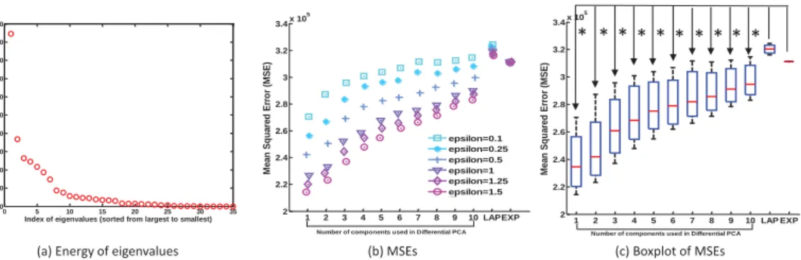
We evaluated our differential PCA-based PPDP by F-norm and compared results with those of Lapla-cian and Exponential mechanisms. The same experiments were repeated 10 times, and we reported the average performance of all three mechanisms in Figure 2.
1 2 3 4 5 6 7 8 9 10 LAPEXP 2 2.2 2.4 2.6 2.8 3 3.2 3.4x 10 5
Number of components used in Differential PCA
M e an S q u ared E rro r ( M S E ) 1 2 3 4 5 6 7 8 9 10 LAP EXP 2 2.2 2.4 2.6 2.8 3 3.2 3.4x 10 5
Number of components used in Differential PCA
M e an S q u ared E rro r ( M S E ) * * * * * * * * * *
(a) Energy of eigenvalues (b) MSEs (c) Boxplot of MSEs
epsilon=0.1 epsilon=0.25 epsilon=0.5 epsilon=1 epsilon=1.25 epsilon=1.5 0 5 10 15 20 25 30 35 0 10 20 30 40 50 60 70 80 90 100 E n erg y ( in p ercen ti le ) o f ei g e n vect o rs i n d exed b y ei g e n val u e s
Index of eigenvalues (sorted from largest to smallest)
Figure 2: Differential PCA is compared to Laplacian (LAP) and Exponential (EXP) mechanisms in terms of the F-norm, i.e., Cumulative mean squared errors (MSE). (a) Energy in percentile carried by eigenvectors sorted by their eigenvalues. (b) Comparison of MSEs between three mechanisms at six different privacy budgets, i.e.,ε=0.1,0.25,0.5,1,1,25,1.5. (c) Boxplots of MSEs. In (b) and (c), we implemented differential PCA-based PPDP with various numbers of components (i.e., 1-10), and all results are averaged from 10 trials. T-test shows that MSEs of PCA are significantly smaller than those of LAP and EXP and PCA (p<0.01), indicated by stars.
The first subfigure indicates that the top 10 eigenvectors carried more than 90% of the entire energy of the data, and there is not much information left for the rest of the eigenvectors. As opposed to the ordinary PCA, the mean squared errors for the differential PCA increase rather than decrease when
more components were used, which implies the noise required for satisfying differential privacy overshadows information carried by additional components.
The second and third subfigures show differential PCA-based PPDP has a clear advantage over Laplacian and Exponential mechanisms, and such differences are statistically significant based on Student-t tests. Indeed, differential PCA outperformed the other two methods in the entire range of component sizes (i.e.,k=1 to 10). Note that we used the strategy introduced in Section 3.1 to convert numerical variables back to categorical ones in order to make the outputs look reasonable.
4.4
Differential LDA Results
4.4.1 Classification performance
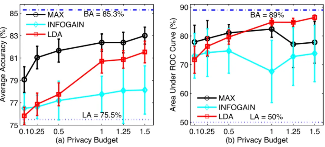
In the first part of this section, we compared the proposed differential LDA with other two data publishing mechanisms targeted at preserving classification information, i.e., DiffGen-INFOGAIN and DiffGen-MAX [25]. First, we use the output of both diffential LDA, DiffGen-INFOGAIN and DiffGen-MAX to train a LDA classifier model and a C4.5 classifier model, respectively. Second, we compare their classification performance in terms of average classification accuracy (ACA) and area under the ROC curves (AUC) based on 10 trials, where we used 2/3 of the records to generate training data and the remaining 1/3 of the records to test the classification performance. To better visualize the performance of the mechanisms, we provide additional measures: error bar is the standard deviation of each data point based on 10 trials,best achievable(BA) andlowest achievable
(LA) performances are the best and lowest possible performances of ACA and AUC measurements given original data or completely generalized data [25], respectively.
0.10.25 0.5 1 1.25 1.5 75 77 79 81 83 85
(a) Privacy Budget
Average Accuracy (%) MAX INFOGAIN LDA BA = 85.3% LA = 75.5% 0.10.25 0.5 1 1.25 1.5 50 60 70 80 90 (b) Privacy Budget
Area Under ROC Curve (%)
MAX INFOGAIN LDA
BA = 89%
LA = 50%
Figure 3: Comparison of (a) the average accuracy and (b) average AUC between DiffGen-INFOGAIN, DiffGen-MAX, and LDA. BA: best achievable; LA: lowest achievable.
Figure 3(a) depicts the ACA among three different methods (i.e., INFOGAIN, DiffGen-MAX, and LDA) with the privacy budgetε=0.1,0.25,0.5,1,1.25,1.5. In addition, BA and LA accuracies are 85.3% and 75.5%, respectively. In Figure 3(a), we can see that the ACA of all three methods increases as the privacy budget increases. Moreover, the ACA of the proposed method out-performs that of DiffGen-INFOGAIN given the privacy budgetε≥0.25, although it is still slightly lower than the ACA of the DiffGen-MAX at high privacy budgets. Furthermore, Figure 3(a) also shows that both the proposed method and DiffGen-MAX have significantly smaller standard devia-tions compared to these of the DiffGen-INFOGAIN. Next, in Figure 3(b), the AUC performances are
0.1 0.25 0.5 1 1.25 1.5 0
5 10 15
(a) Privacy Budgets
Average Entropy Raw Data LDA INFOGAIN MAX 0.1 0.25 0.5 1 1.25 1.5 0 0.5 1 1.5 2 2.5 3 (b) Privacy Budgets Average KL Divergence LDA INFOGAIN MAX
Figure 4: Comparison of the capability of information preservation among DiffGen-INFOGAIN, DiffGen-MAX, and LDA: (a) the average entropy of released data; (b) the average KL divergence between released data and the original data.
also studied to measure the classification performance of the three different anonymization methods. The AUCs of the proposed method are clearly higher than these of the other two methods, when the privacy budget is larger than 0.5. More important, our proposed method always offers the lowest standard deviation for all different budgets among all three methods. The experimental results sug-gested that the proposed differential LDA method achieves a comparable ACA with DiffGen-MAX, but higher AUC on average and a lower AUC standard deviation.
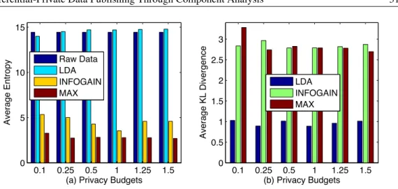
4.4.2 Information preservation
In the second part, we also compared all the three methods in terms of information preservation. We measure the preserved information of these mechanisms by two information theoretic metrics: entropy and Kullback-Leibler (KL) divergence [33]. In Information Theory, the entropy provides a measure of how much information the data contain. A larger entropy for the released data implies a greater amount of information that a released data might contain, however, does not indicate how relevant such infromation is about the original data. The KL divergence (a.k.a. relative entropy) was introduced to measure the differenceDKL(P||Q)between the distribution of released dataPand that
of the original dataQ, whereDKL(P||Q)is a non-negative metric withDKL(P||Q) =0 if and only if
P=Q.
Figure 4(a) shows the entropies of released data by using DiffGen-INFOGAIN, DiffGen-MAX and the proposed differential LDA, where the entropy of original data is given as a reference. We can see that the entropy obtained by the proposed method is similar to that of the original data, whereas the entropies of the other two methods (i.e., DiffGen-INFOGAIN and DiffGen-MAX) are quite lower than that of the original data. In other words, the amount of information preserved by our proposed anonymization method is comparable to that of the original data, while the amount of released information in DiffGen-INFOGAIN and DiffGen-MAX methods are only about 30% and 20% of the original data, respectively. These results indicate that both the DiffGen-INFOGAIN and DiffGen-MAX methods merely intend to preserve useful information for classification purpose. In contrast, the proposed method could preserve an equivalent amount of information as the original data, which offers greater usability for general-purpose data mining tasks other than classification.
methods is relevant to the original data, in terms of KL divergence. Figure 4(b) shows that the proposed method achieves the minimum average KL divergence among all three anonymization methods, where the KL divergence of the proposed method is only about one thirds of the other two methods. This shows that differential LDA outperforms the other two methods, as it maintains a more similar distribution in the released data, as well as preserves a larger amount of information.
5
Conclusions
In this paper, we proposed two novel mechanisms for privacy preserving data publishing that achieve
ε-differential privacyand provide better utility than the existing techniques. Two mechanisms,
dif-ferential Principle Component Analysis and difdif-ferential Linear Discriminant Analysis were studied in this paper. The former method serves as a general-purpose data dissemination tool that guarantees better utility (i.e., lower error) when compared to Laplacian and Exponential mechanisms, that use the same privacy budget. The method is applicable to data dissemination for classification purposes. Through theoretically justification and experimental comparisons, we showed that the proposed pri-vacy preserving data publishing mechanisms are more effective than the state-of-the art alternatives in retaining data utility.
6
Acknoledgements
XJ, LZ, SW and LO-M were funded in part by the NIH grants K99LM011392, UH2HL108785, U54HL108460, UL1TR00010003 and the AHRQ grant R01HS019913.
References
[1] D. Alemayehu, R. J. Sanchez, and J. C. Cappelleri, “Considerations on the use of patient-reported out-comes in comparative effectiveness research,”Journal of Managed Care Pharmacy, vol. 17, no. 9 Suppl A, pp. S27–33, 2011.
[2] N. Adam, T. White, B. Shafiq, J. Vaidya, and X. He, “Privacy preserving integration of health care data.,”
AMIA Annual Symposium proceedings, pp. 1–5, Jan. 2007.
[3] K. El Emam, “Risk-Based De-Identification of Health Data,”IEEE Security & Privacy Magazine, vol. 8, pp. 64–67, May 2010.
[4] N. Mohammed, B. C. M. Fung, P. C. K. Hung, and C.-K. Lee, “Centralized and distributed anonymization for high-dimensional healthcare data,”ACM Transactions on Knowledge Discovery from Data, vol. 4, pp. 1–33, Oct. 2010.
[5] C. Dwork, “A firm foundation for private data analysis,”Communications of the ACM, vol. 54, pp. 86–95, Jan. 2011.
[6] N. R. Adam and J. C. Worthmann, “Security-control methods for statistical databases: a comparative study,”ACM Computing Surveys, vol. 21, pp. 515–556, Dec. 1989.
[7] B. C. M. Fung, K. Wang, R. Chen, and P. S. Yu, “Privacy-Preserving Data Publishing: A survey of recent developments,”ACM Computing Surveys, vol. 42, pp. 1–53, June 2010.
[8] R. Sarathy and K. Muralidhar, “Evaluating Laplace noise addition to satisfy differential privacy for nu-meric data,”Transactions on Data Privacy, vol. 4, no. 1, pp. 1–17, 2011.
[9] K. Chaudhuri and C. Monteleoni, “Privacy-preserving logistic regression,” inNeural Information Pro-cessing Systems, pp. 289–296, 2008.
[10] L. Sweeney, “k anonymity: A model for protecting privacy,”International Journal of Uncertainty Fuzzi-ness and Knowledge Based Systems, vol. 10, no. 5, pp. 557–570, 2002.
[11] A. Machanavajjhala, D. Kifer, J. Gehrke, and M. Venkitasubramaniam, “l-diversity: privacy beyond k-anonymity,”ACM Transactions on Knowledge Discovery from Data, vol. 1, pp. 3–es, Mar. 2007. [12] R. Chi-Wing, J. Li, A. W.-C. Fu, and K. Wang, “(α, k)-Anonymity,” inProceedings of the 12th ACM
SIGKDD international conference on Knowledge discovery and data mining, (New York, NY), pp. 754– 761, 2006.
[13] B. C. M. Fung, K. Wang, and P. S. Yu, “Anonymizing classification data for privacy preservation,”IEEE Transactions on Knowledge and Data Engineering, vol. 19, pp. 711–725, May 2007.
[14] K. LeFevre, D. J. DeWitt, and R. Ramakrishnan, “Workload-aware anonymization techniques for large-scale datasets,”ACM Transactions on Database Systems, vol. 33, pp. 1–47, Aug. 2008.
[15] R. C. W. Wong, A. W. C. Fu, K. Wang, and J. Pei, “Minimality attack in privacy preserving data pub-lishing,” inProceedings of the 33rd international conference on Very large data bases, (Vienna, Austria), pp. 543–554, 2007.
[16] S. R. Ganta, S. Kasiviswanathan, and A. Smith, “Composition attacks and auxiliary information in data privacy,” inProceedings of the ACM International Conference on Knowledge Discovery and Data Mining, pp. 265–274, 2008.
[17] D. Kifer, “Attacks on privacy and de Finetti’s Theorem,” in Proceedings of the ACM Conference on Management of Data, (Providence, RI), pp. 127–138, 2009.
[18] R. C. W. Wong, A. W. C. Fu, K. Wang, Y. Xu, and P. S. Yu, “Can the utility of anonymized data be used for privacy breaches?,”ACM Transactions on Knowledge Discovery from Data, vol. 5, pp. 1–24, Aug. 2011.
[19] I. Dinur and K. Nissim, “Revealing information while preserving privacy,” inProceedings of the twenty-second ACM SIGMOD-SIGACT-SIGART symposium on Principles of database systems, (New York, NY), pp. 202–210, 2003.
analy-sis,” inTheory of Cryptography, vol. 3876, pp. 265–284, 2006.
[21] R. Bhaskar, S. Laxman, A. Smith, and A. Thakurta, “Discovering frequent patterns in sensitive data,” inProceedings of the 16th ACM SIGKDD international conference on Knowledge discovery and data mining, (New York, NY), pp. 503–510, 2010.
[22] A. Friedman and A. Schuster, “Data mining with differential privacy,” inProceedings of the 16th ACM SIGKDD International Conference on Knowledge Discovery and Data Mining, (New York, NY), pp. 493– 502, 2010.
[23] X. Xiao, G. Wang, and J. Gehrke, “Differential privacy via wavelet transforms,” inIEEE Transactions on Knowledge and Data Engineering, vol. 23, pp. 1200–1214, Aug. 2011.
[24] M. Hay, V. Rastogi, G. Miklau, and D. Suciu, “Boosting the accuracy of differentially-private histograms through consistency,” inProceedings of the International Conference on Very Large Data Bases, vol. 3, pp. 15–22, Apr. 2009.
[25] N. Mohammed, R. Chen, B. C. Fung, and P. S. Yu, “Differentially private data release for data min-ing,”Proceedings of the 17th ACM SIGKDD international conference on Knowledge discovery and data mining, p. 493, 2011.
[26] A. Blum, C. Dwork, F. McSherry, and K. Nissim, “Practical privacy: the sulq framework,” in Proceed-ings of the twenty-fourth ACM SIGMOD-SIGACT-SIGART symposium on Principles of database systems, pp. 128–138, ACM, 2005.
[27] C. Dwork, “Differential privacy,” inInternational Colloquium on Automata, Languages and Program-ming, vol. 4052, pp. 1–12, 2006.
[28] Y. Li, Z. Zhang, M. Winslett, and Y. Yang, “Compressive mechanism: Utilizing sparse representation in differential privacy,” inProceedings of the 10th annual ACM workshop on Privacy in the electronic society, pp. 177–182, ACM, 2011.
[29] F. McSherry, “Privacy integrated queries: an extensible platform for privacy-preserving data analysis,” inProceedings of the 35th SIGMOD international conference on Management of data, (Providence, RI), pp. 19–30, ACM, 2009.
[30] F. McSherry and K. Talwar, “Mechanism design via differential privacy,” inProceedings of the 48th Annual IEEE Symposium on Foundations of Computer Science, (Providence, RI), pp. 94–103, Oct. 2007. [31] A. Blum and K. Ligett, “A learning theory approach to non-interactive database privacy,” inProceedings of the 40th annual ACM symposium on Theory, (Victoria, British Columbia, Canada), pp. 609–618, 2008. [32] A. Asuncion and D. J. Newman, “UCI machine learning repository,” 2007.