Two-dimensional Tissue Image Reconstruction
Based on Magnetic Field Data
Jarmila D
Ě
DKOVÁ, Ksenia OSTANINA
Dept. of Theoretical and Experimental Electrical Engineering, Brno University of Technology, Kolejní 2906/4, 612 00 Brno, Czech Republic
[email protected], [email protected]
Abstract. This paper introduces new possibilities within two-dimensional reconstruction of internal conductivity distribution. A new algorithm for the conductivity recon-struction was developed. This algorithm utilizes the inter-nal current information with respect to corresponding boundary conditions and the induced magnetic field meas-ured outside the object. A series of computer simulations has been conducted to assess the performance of the pro-posed algorithm within the process of estimating electrical conductivity changes in the lungs, heart, and brain tissues captured in two-dimensional piecewise homogeneous chest and head models. The reconstructed conductivity distribu-tion using the proposed method is compared with that using a conventional method based on Electrical Imped-ance Tomography (EIT). The acquired experience is dis-cussed and the direction of further research is proposed.
Keywords
Impedance tomography, magnetic resonance, image reconstruction, inverse problem, finite element method.
1.
Introduction
An image reconstruction technique based on imped-ance tomography has been an active research topic since the early 1980s. Since this time, there have been significant efforts to produce cross-sectional images of impedivity (conductivity and permittivity) distribution inside the hu-man body using boundary measurements of current-voltage data. This technique is commonly called Electrical Imped-ance Tomography [1]. An interesting overview of different possibilities within general tomography techniques and their recent applications can be found in [2], [3].
Based on many other published studies, it is possible to say that medical imaging has been one of the prominent applications of EIT. Biological tissues have different elec-trical properties that change with cell concentration, cellu-lar structure and density, molecucellu-lar composition, mem-brane characteristics, and other factors. Consequently, the
properties reflect structural, functional and pathological conditions of the tissue and can provide valuable diagnos-tic information. Many researchers have tested out the elec-trical conductivity of tissues and shown that there is a dif-ference in conductivity between a normal and a fatigued tissue and between a healthy and a pathologic tissue [4]. In [5], the author has used the degree of resistance of the brain tissue to an electric current as a means of differenti-ating between the normal brain and a tumor tissue on the operating table. The conductivity of normal tissues has been measured experimentally; other details can be found e.g. in [6-8]. Further, we will focus on conductivity only since it constitutes an important physical index that can indicate conditions of tissues or organs.
In recent years, numerous studies have attempted to develop algorithms which reconstruct cross-sectional con-ductivity images from Magnetic Resonance Electrical Impedance Tomography (MREIT) [9-12]. The question of using the MREIT for recovering the interior object con-ductivity when the current is applied on its boundary is very often discussed. The injecting currents produce a magnetic field which has been used together with meas-ured voltage-current data for recovering the conductivity distribution. While the EIT suffers from the ill-posed nature of the corresponding inverse problem, the MREIT has been presented as a conductivity imaging modality providing images with better spatial resolution and accu-racy. Unfortunately, by injecting current through surface electrodes we measure only one component of the induced internal magnetic flux density using an MRI scanner. In order to reconstruct the conductivity distribution inside the imaging object, most algorithms in the MREIT have re-quired multiple magnetic flux density data during the in-jection of at least two independent currents [13].
In this paper, one direct method for reconstructing the internal isotropic conductivity is proposed; it is necessary to know only one component of magnetic flux density data when injecting one current into the imaging object through a single pair of surface electrodes. Firstly, the proposed method reconstructs the density of a projected current, which is a uniquely determined current from the measured one component of the magnetic flux density outside the imaging object. Using the relation between the electric
field and the current density, based on Ohm’s law, the additional condition can be introduced to an implicit matrix system for the determination of internal conductivity dis-tribution.
Here, the described techniques utilize internal infor-mation on the induced magnetic field in addition to the boundary current-voltage measurements to produce images of internal current density and conductivity distributions. In this paper, a new way to obtain these distributions with-out the knowledge of voltage data on the boundary of the proposed testing object is presented. It is shown that this technique can be applied conveniently to identify the loca-tion of regions with different conductivity values or to identify local changes of these values.
2.
Basic Theory
The current density J in a linear medium with the interior electrical conductivity can be obtained from the electric field E or the corresponding potential distribu-tion U
gradU
J E . (1)
The impedance tomography problem is a recovery of the conductivity distribution satisfying the continuity equation
divJ 0.
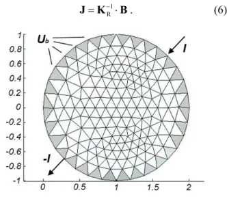
Now we consider the two-dimensional numerical model with NE linear triangle elements with NU nodes (see e.g.
Fig. 1). We approximate (1) from nodal values Ui using
linear approximation functions Ni(x, y) on a grid of linear
triangular finite elements
U 1 ( , ) ( , ) N i i i U x y U N x y
. (2)Then we can describe the current density J(e)(x, y) on each
element (e) by (3) 3 1 ( , ) grad ( , ) e e e e j j j x y
U N x y
J (3) where σ(e) and Nj(e)(x, y) are the conductivity and the linear approximation function on element (e). We now consider that the current is injected into a two-dimensional electri-cally conductive object. The induced magnetic flux density
B corresponding to J can be described using the Biot-Savart law. If the magnetic flux density B due to the injec-tion current is known from the measurements, an image of the corresponding internal current density distribution J
can be obtained from, for example, Ampere´s law 0
rot
/
J
B
.This method naturally requires the knowledge of all com-ponents of a magnetic field; therefore, in the following text, we will propose a simpler procedure. The magnetic
field Bi can be calculated numerically in the general point given by coordinates [xi, yi, zi] using the Biot-Savart law and the principle of superposition
0 3 1
4
E N j ij i j j ijV
R
J
R
B
(4)where NE is the number of elements, Jj is the current den-sity on element j, ∆Vj represents the volume of element j, and Rij represents the distance between the centre [xj, yj, zj] of element j and the point [xi, yi, zi]. The components of magnetic field can be expressed
0 0 3 , 3 , 4 R 4 R yj zij j xj zij j xij yij ij ij J R V J R V B
B
0 3 4 R xj yij yj xij j zij ij J R J R V B
.It is obvious that, to obtain the NE pair of Jx and Jy compo-nents of a current density, we have to know either the same number of Bx and By components or the double number of
Bz component of a magnetic field. Let us suppose we know the 2 NE values of Bz; then, each of them is given
E E 1 ( ) , 1,..., 2 N zi Ryij xj Rxij yj j B K J K J i N
.The matrix notation of 2NE algebraic equations is
R R x y x z y J K K B J KR J B. (5)From (5) we can obtain the source current density distribution very easily
1 R
J K B. (6)
Fig. 1. An arrangement for numerical simulations.
The conductivity reconstruction process is usually presented as the minimization of the primal objective function U(), which can be based on the Method of
2 2
U M FEMb 1 1 , 2 2
U L U U U . (7)Here, UM, UFEMb are the measured and calculated voltages
on the object boundary, α is a regularization parameter, L
is a suitable regularization matrix, is the unknown vector of conductivity distribution inside the object. After applying the Newton-Raphson method, the iteration procedure can be obtained
T T 1 T T 1 ( ) ( ) i i i i
i
i
i σ σ J J L L J U L Lσ .Here, i is the i-th iteration and Jis the Jacobian
FEMb( ) i
U J
.This way we look for such conductivity distribution which minimizes the difference between the measured and calcu-lated voltages on the boundary UM, UFEMb. The size of UM
depends on the number of measuring electrodes and the number of current patterns.
However, the above-described solution is not the only one possible. We can also minimize the difference between current densities JM and JFEM on the elements. The JFEM
vector corresponds to calculated voltage UFEM and it can be
computed using UFEM and (3). The JM vector can be
ob-tained from the measured value of magnetic field using (6). Then, the object function K() can be described
2 2
K M FEM 1 1 , 2 2
J L J J J . (8) The meaning of parameters α and L is the same as that mentioned above. If we apply the Newton-Raphson method, we obtain the iteration procedureT T 1 T T
1 ( I I ) ( I )
i i i i
i
i
iσ σ J J L L J J L Lσ .
Here, i is the i-th iteration and JI is the corresponding
Jacobian
E E E
E FEM1 FEM1 FEM1
1 2
FEM I
FEM FEM FEM
1 2 ; ; ... ( ) : : : ; ; ... E N N N N N
J J J J J J J J
.In the following part, an example is shown of the magnetic field distribution, the corresponding surface cur-rent density distribution, and the influence of nonhomoge-neity inside the tested sample. From the difference of cur-rent density J in the samples without nonhomogeneity and with nonhomogeneity, we can obtain the conductivity dis-tribution using the conditions on the boundary between two media with different conductivities. The forward solution system equation can be described using the Finite Element
Method
FEM ( ) ( )
K U F .
The forward operator UFEM 1 FEM( ) ( )
U K F
can be calculated more effectively if we know the conduc-tivities on all boundary elements. In this case, we can recalculate very easily, using (3), the potential Ub at the
corresponding Nb boundary nodes, see Fig. 1. This means
that the number of equations NU for the forward solution
can be reduced to (NU – Nb) equations and that we can save
the computational time.
3.
Numerical
Simulations
The basic arrangements of the average conductivity distribution of healthy tissues in the slice of a chest and a head can be seen in Fig. 2 (NE = 300, NU= 167) and
Fig. 3 (NE = 2360, NU = 1237). The finite element mesh for
each simulation model was created by using program Ansys 12.0; then regions representing the different types of biological tissues were chosen. The chest model has 20 cm diameter. The width of head model is 14.40 cm and its height is 19.95 cm.
Fig. 2. A chest model for the reconstruction of conductivity changes in heart or lungs.
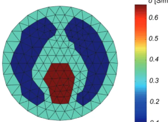
Fig. 3. A head model for the reconstructions of conductivity changes.
In Fig. 2, the simplified model represents the chest with just three homogeneous isotropic layers: lung (dark blue color), heart (brown color) and body tissue (blue color). The next simulation model presented in Fig. 3 is a simplified model of the human head, which consists of four homogeneous isotropic layers: gray and white matters (orange and blue colors), the skull (dark blue color), and the scalp (brown color). Therefore, it is necessary to know only values of average regional conductivities of chest tissues and head tissues of corresponding models for reali-zation of image reconstruction.
The knowledge and the easy monitoring of tissue conductivity changes are very useful and crucial in clinical medicine for diagnostics and during the therapy. The con-ductivity values of different biological tissues used for the following simulations are presented in Tab. 1; these values were taken from previously published literature on this topic, see [14]. Tissue Conductivity [S/m] Heart 0.667 Lung 0.100 Body tissue 0.333 Gray matter 0.352 White matter 0.147 Skull 0.087 Scalp 0.435 Blood 0.900 Blood clot 0.300 Tumor 0.956
Tab. 1. The electrical conductivity of human tissues.
Fig. 4. Thedetection of blood clots in lungs.
Fig. 5. The detection of a blood clot in a heart.
The first reconstruction results of conductivity changes detection are presented in the Fig. 4 and 5. The final conductivity image with the detection of blood clot regions in lungs is shown in Fig. 4; original blood clot regions are represented by three triangle elements inside lungs with conductivity 0.3 S/m.
The result in Fig. 5 demonstrates the detection of a blood clot in a heart; in this case the original blood clot region is represented by three elements inside a heart with conductivity 0.3 S/m.
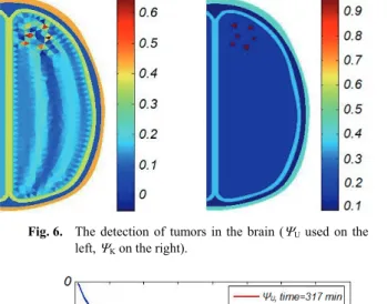
It is well known that the conductivity of a tumor tis-sue is significantly greater than that of a normal tistis-sue. The conductivity imaging techniques could be potentially use-ful also for early diagnosis of tumors. However, in order to visualize any tumor at its early stage, the reconstructed conductivity image must be accurate with a high spatial resolution of any arbitrary tumor size and locations.
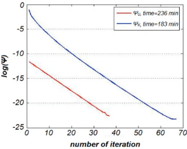
Fig. 6 presents two different reconstruction results related to the detection of several small brain tumors. The original brain tumor distribution is represented by six ele-ments with conductivity 0.956 S/m. In the figure, the left section shows the final conductivity distribution when the object function U given by (7) was optimized (old way),
and the right section contains the same result when the K
given by (8) was optimized (new way). The behavior of both object functions during the iteration process is shown in Fig. 7.
Fig. 6. The detection of tumors in the brain (U used on the
left, K on the right).
The next example shows another possible method of brain tumors detection. In this case, the filter reducing the number of unknowns was introduced to both tested algo-rithms. Fig. 8 presents a comparison between results obtained through a reconstruction based on the U
optimi-zation (left) and results achieved by means of the K
optimization (right). The behavior of object functions U
and K is, during the reconstruction, similar to the
de-scription shown in Fig. 7. The algorithm run time was in both cases significantly reduced by the application of a suitable filter during the reconstruction process [15]; it was reduced three times for an old algorithm and fifteen times for a proposed algorithm.
Fig. 8. The detection of three brain tumors (U used on the
left, K on the right).
The last example demonstrates the applicability of the new algorithm for detection of brain blood clot. In this case, the defect represents the simplified model of blood clot. Fig. 9 presents a comparison between results obtained through a reconstruction based on the U optimization
(left) and results achieved by means of the K optimization
(right). In Fig. 10, the object functions U and K are
compared during the reconstruction. All obtained recon-struction results show that the proposed algorithm stably and reliably determines the conductivity changes in an imaging slice.
Fig. 9. The detection of a blood clot in the brain (U used on
the left, K on the right ).
Fig. 10. Objective functions during the detection of a blood clot.
All above-presented simulations were obtained under the condition that the size of UM was 380 and size of JM
was 789.
The high degree of accuracy was achieved by apply-ing the new algorithm, namely the same conductivity dis-tribution as original ones was obtained as a result of imag-ing by this algorithm in all these cases.
4.
Conclusion
A new approach to the two-dimensional reconstruc-tion of conductivity distribureconstruc-tion based on using one com-ponent of magnetic flux density data was proposed. The magnetic field required was created by injecting a current into the imaging object through a single pair of surface electrodes. Then, the modified object function K was used
for the optimization instead of the usual object function
U.
We can also express the object function as follows:
2 2 B M FEM 1 1 . 2 2
B B LHere, BM, BFEM are the measured and calculated values of
magnetic flux density outside the given object. The algo-rithm based on the minimization of the object function B
was also tested. In comparison with the case when the object function K is minimized, the quality of obtained
reconstruction results was somewhat worse and this tech-nique was more time-consuming.
Finally, the reduction of the number of unknowns (in accordance with a suitable filter based on, for example, the knowledge of conductivity on some elements) was intro-duced to the forward solution of the basic iteration process.
The applicability of this new feasible algorithm was verified on different numerical examples. The representa-tive results were presented in this paper; they confirm that the proposed algorithm can stably and effectively deter-mine the internal conductivity distribution and also con
ductivity changes in an imaging slice. The new approach is based on the use of magnetic field data, which can be obtained by a wireless measurement. This is the main advantage compared to the EIT approach.
The resolution of new method depends on the density of mesh, namely the number of unknown σ(e). Therefore,
stability and convergence of the reconstruction process will be ensured, if the number of measured values (voltage or components of magnetic field) is equal to or greater than the number of unknown. Unfortunately, the proposed way is not applicable to 3D image reconstruction of conductiv-ity distribution.
The electrical properties of healthy and ill tissues have been studied for a long time. It is possible to say that e.g. the dielectric properties of the tumor cells showed higher permittivity and conductivity values than a homolo-gous healthy tissue [16]. Further investigation will be therefore focused on the main goal - to introduce in the proposed algorithm the possibility of permittivity image reconstructions.
Acknowledgements
The research described in the paper was financially supported by the research program MSM 0021630513.
References
[1] HOLDER, D. S. Electrical Impedance Tomography. Philadelphia: IOP Publishing, 2005.
[2] SIKORA, J., WÓJTOWICZ, S. Industrial and Biological Tomo-graphy. Theoretical Basis and Applications. Warsaw: Electrotech-nical Institute, 2010.
[3] SANKOWSKI, D., SIKORA, J. Electrical Capacitance Tomogra-phy. Theoretical Basis and Applications. Warsaw: Electrotechnical Institute, 2010.
[4] CRILE, G. W., HOSMER, H. R., ROWLAND, A. F. The electrical conductivity of animal tissue under normal and pathological conditions. American Journal of Physiology, 1922, vol. 60, no. 1, p. 59 - 106.
[5] MEYER, A. W. Method for detecting brain tumors in the trepanation by electrical resistance measurement (Methode zum Auffinden von Hirntumoren bei der Trepanation durch elektrische Widerstandsmessung). Zentralblatt fur Chirurgie, 1921, no. 48, p. 1824 – 1826 (in German).
[6] FOSTER, K. R., SCHWAN, H. P. Dielectric properties of tissues and biological materials: a critical review. Critical Reviews in Biomedical Engineering, 1989, vol. 17, no. 1, p. 25 - 104.
[7] GEDDES, L. A., BAKER, L. E. The specific resistance of biological materials - a compendium of data for the biomedical engineer and physiologist. Medical and Biological Engineering and Computing, 1967, vol. 5, no. 3, p. 271 - 293.
[8] LAW, S. K. Thickness and resistivity variations over the upper surface of the human skull. Brain Topography, 1993, vol. 6, no. 2, p. 99 - 109.
[9] SEO, J. K., KWON, O., WOO, E. J. Magnetic resonance electrical impedance measurement tomography (MREIT): conductivity and current density imaging. Journal of Physics: Conference Series,
2005, vol. 12, p. 140 - 155.
[10] JEON, K., LEE, C.-O., WOO, E. J., KIM, H. J., SEO, J. K. MREIT conductivity imaging based on the local harmonic Bz algorithm:
animal experiments. Journal of Physics: Conference Series, 2010, vol. 224, no. 1, p. 1 - 4.
[11] LEE, T. H., NAM, H. S., LEE, M. G., KIM, Y. J., WOO, E. J., KWON, O. I. Reconstruction of conductivity using the dual-loop method with one injection current in MREIT. Physics in Medicine and Biology, 2010, vol. 55, no. 24, p. 7523 - 7539.
[12] KWON, O., LEE, J. Y., YOON, J. R. Equipotential line method for magnetic resonance electrical impedance tomography. Inverse Problems, 2002, vol. 18, p. 1-12.
[13] ZHANG, X., YAN, D., ZHU, S., HE, B. Noninvasive imaging of head-brain conductivity profiles. IEEE Engineering in Medicine and Biology Magazine, 2008, vol. 27, no. 5, p. 78 - 83.
[14] MIKLAVČIČ, D., PAVŠELI, N., HART, F. X. Electric Properties of Tissues. Wiley Encyclopedia of Biomedical Engineering. John Wiley & Sons, 2006.
[15] DĚDKOVÁ, J., OSTANINA, K. Implementation of fuzzy filters in EIT image reconstructions. Acta Technica ČSAV, 2011, vol. 56, no. 2, p. 207 - 216.
[16] GHANNAM, M. M., EL-GEBALY, R. H., GABER, M. H., ALI, F. F. Inhibition of Ehrlich tumor growth in mice by electric interference therapy (in vivo studies). Electromagnetic Biology and Medicine, 2002, vol. 21, no. 3, p. 255 - 268.
About Authors ...
Jarmila DĚDKOVÁ was born in Znojmo in 1959. She received her master’s degree in Electrical Engineering from Brno University of Technology in 1983. Her profes-sional and current research interests are directed towards the development of algorithms for the electromagnetic field modeling, optimization and effective solution of inverse problems.
Ksenia OSTANINA was born in Izhevsk in 1987. She received her master’s degree in Electrical Engineering from Izhevsk State Technical University in 2009. Her re-search is focused on numerical methods for image recon-structions of biological tissues conductivity.