How To Improve Supply Chain Performance

IMPROVING SUPPLY CHAIN

PERFORMANCE THROUGH

BUYER COLLABORATION

∗

School of Industrial and Systems Engineering Georgia Institute of Technology

765 Ferst Drive Atlanta, GA 30332-0205 {pgriffin,pinar,secil}@isye.gatech.edu

Abstract We study alternative buyer strategies in markets where procurement costs are effected by economies of scale in the suppliers’ production costs and by economies of scope in transportation. We consider buyer strategies with different levels of collaboration, namely, (i) no collabora-tion among buyers or buyer divisions, (ii) internal collaboracollabora-tion among the purchasing organizations of the same buyer enabled by an internal intermediary, and (iii) full collaboration among multiple buyers enabled by a third party intermediary. We test these buyer strategies under different market conditions and provide insights on when intermediaries have a significant impact on the economic value as well as the buyer surplus.

1.

Introduction

In recent years, we have seen a rapid growth of electronic markets (e-markets or exchanges) which bring buyers and suppliers together and enable many-to-many transactions. Depending on who owns and op-erates them, we can divide e-markets into two categories (Elmaghraby

∗_{Acknowledgement: Pınar Keskinocak is supported by NSF Career Award DMI-0093844.}

This research is also supported in part by NSF grant EEL-9802942. The authors are grateful to an anonymous referee and Joseph Geunes for their constructive feedback throughout the revision of this paper.

and Keskinocak (2002)): (1) Private e-markets that are owned by a company (commonly referred to as a private trading exchange (PTX)) or a group of companies (co-op or consortia exchanges (CTX)) who are either a buyer(s) or seller(s) in the market, and (2) independent trading exchanges (ITX) that are owned and operated by an indepen-dent entity (i.e., not wholly/partially owned by a buyer or seller in the market). Examples of such e-markets are GE Plastics (geplastics.com), which is a PTX, Transplace (transplace.com), which is a consortium ex-change formed by the merger of logistics business units of the six largest publicly-held truckload carriers, and Chemconnect (chemconnect.com), an ITX specializing in chemicals and plastics. The benefits of e-markets compared to traditional channels include reduced transaction costs and access to a larger base of potential buyers and suppliers.

Although e-markets began with great fanfare, they have not, at least so far, lived up to their advanced billing. This is especially true for ITXs. Among the reasons why ITXs have failed are privacy concerns, and more importantly, the sellers’ concerns about being compared solely on price. PTXs, on the other hand, have gained popularity, as more companies strive to streamline their interactions with their supply chain partners. PTXs have the advantage of giving more control to the owner com-pany and enabling information-sharing and other types of collaboration among participants. In order for ITXs and CTXs to be successful, they should offer more than decreased transaction costs or one-stop shopping convenience. All types of exchanges would benefit significantly from col-laboration and decision-support tools for the trading process (Stackpole (2001)), (Keskinocak and Tayur (2001)).

In many companies, purchasing is done by multiple functional divi-sions (or purchasing organizations within the company) which either act independently or have minimal interaction with each other. For example, until very recently purchasing was done locally by managers at each of the Dial Corp.’s sites. It was typical for buyers at one fa-cility to buy the same raw material as a buyer at another Dial plant from two different suppliers at different prices. This approach was in-effective in taking advantage of Dial’s volume and corporate-wide buy-ing power (Reilly (2002)). Similarly, until 1997, purchasbuy-ing at Siemens Medical Systems was done locally, where buyers at Siemens’ ultrasound, electromedical, computer tomography, magnetic resonance imaging and angiography divisions independently bought the components and mate-rial that their individual plants needed and rarely communicated with each other. There was no pooling of component demand for leveraging purposes (Carbone (2001)). Recently both companies have moved with

great success towards centralized procurement, which allows collabora-tion among internal purchasing units.

In addition to internal collaboration within a company, there is also a growing interest in collaboration among different companies on vari-ous supply chain functions, such as demand forecasting, product design, transportation, and procurement. Such inter-company collaboration is sometimes enabled by market intermediaries in the industry. For ex-ample, the Internet-based logistics network, Nistevo, consolidates orders from multiple shippers and creates round-trip or dedicated tours. This reduces the costs of the carriers due to better utilization of truck ca-pacity and in turn results in lower prices for the shippers (Strozniak (2001)). For example, Land O’Lakes Inc. has saved $40,000 a month by coordinating its shipping routes with companies such as Georgia-Pacific (Keenan and Ante (2002)).

Motivated by the current practices and the potential benefits of col-laborative procurement, we study the performance of buyer strategies with different levels of collaboration under various market conditions. We assume buyers have multiple functional divisions responsible for pur-chasing. To analyze the benefits of collaboration, we study procurement

strategies under three collaboration models: (i)No collaboration: Buyer

divisions and suppliers trade through traditional sales channels, via one-to-one transactions. No information flow or collaboration exists among

the functional divisions of a buyer or among multiple buyers. (ii)

Inter-nal collaboration: Functional divisions of a buyer collaborate internally.

(iii)Full collaboration: A third party intermediary enables collaboration

among different buyers and allows the participants to achieve benefits from both economies of scale and scope due to reduced fixed produc-tion and transportaproduc-tion costs. We refer to the total set of trades among

the buyers and suppliers as a matching. The three models are shown

in Figure 1.1. Note that the connectivity requirements (and hence, re-lated transaction or search costs) between the buyers and the suppliers decrease as the collaboration level increases.

We conduct numerical experiments to analyze the effectiveness of buyer strategies under different market conditions. We characterize the markets based on three main attributes: the capacity level compared to the total demand in the market, the sellers’ relative fixed and variable production costs, and the relative fixed and variable transportation costs. We compare the strategies based on the following performance measures: the percentage of satisfied demand, total surplus of the buyers, average surplus per unit, and the average cost per unit. Buyer surplus can be regarded as some form of buyer profit, which we will formally define in Section 3.

Figure 1.1. Three models of collaboration among buyers and buyer divisions

This chapter is organized as follows. In Section 2 we provide a liter-ature review. Alternative buyer strategies with different collaboration levels are presented in Section 3. Experimental results and managerial insights are given in Section 4 and Section 5 followed by a concluding discussion in Section 6.

2.

Literature Review

Interactions among participants of a supply chain can be analyzed along several directions. One line of related research focuses on de-centralized versus shared information. When the information is decen-tralized, studies are primarily on constructing different mechanisms to enable coordination in a two-stage setting and to eliminate inefficiencies stemming from double marginalization. Cachon and Zipkin (1999) and Lee et al. (2000) analyze coordination mechanisms in the form of rebates or transfer payments. Weng (1995) considers a system where coordina-tion is established through quantity discounts and franchise fees. Jin and Wu (2001) study supply chain coordination via transfer payments in the presence of e-market intermediaries. See Cachon (2003) for an analysis of coordinating contracts under different supply chain settings. Another line of research focuses on collaboration. Internet and tech-nology have made information sharing possible at every stage, and this leads to different collaborative efforts in supply chains. Examples include vendor managed inventory (VMI), just-in-time distribution (JITD), and collaborative planning, forecasting and replenishment (CPFR), in which trading partners such as vendors and retailers collaborate vertically. In VMI systems the vendor is given autonomy in replenishing the retailer’s

orders and in turn manages the retailer’s inventory with fewer stockouts and at low levels. In a pilot effort of CPFR, Wal-Mart and vendors Lucent and Sara Lee shared event and point of sales information to jointly forecast sales in 1997 (http://www.cpfr.org). There is a growing interest in supply chain literature on analyzing the benefits of VMI in supply chains, for example see Cetinkaya and Lee (2000), and Cheung and Lee (2002). Relatively little research exists on collaboration through forecasting. Aviv (2001) studies the benefits of collaborative forecasting with respect to decentralized forecasting.

Horizontal collaboration differs from vertical in the sense that it con-siders collaboration among only those on the buyer or supplier side. Horizontal coordination and collaboration in the supply chain enabled by quantity discounts is studied by Gurnani (2001) in a single supplier two buyer setting. Some existing research considers the interaction of buyers and suppliers from a resource allocation perspective. Ledyard, Banks and Porter (1989) test allocation mechanisms with uncertain re-sources and indivisible demand. The results indicate that high efficiency could be obtained if collaboration is enabled among buyers. To the best of our knowledge there has not been much research on the loss of effi-ciency due to lack of horizontal collaboration. In this paper, we study the interaction between multiple buyers and multiple suppliers, where horizontal collaboration is enabled by a central mechanism (or interme-diary).

A similar problem is studied by Kalagnanam, Davenport and Lee (2001), where the motivation came from electronic markets in the paper and steel industries. The authors consider an e-market in which buyers and suppliers submit bid and ask prices for multiple units of a single product. They show that the problem of determining the clearing price and quantity under different assignment constraints can be solved in polynomial time when demand is divisible, but is NP-hard when demand is not divisible.

We extend the work of Kalagnanam, Davenport and Lee (2001) in several directions. We consider multiple products, rather than a single product, where each supplier needs to decide how to allocate its limited capacity among these multiple products. Furthermore, we consider fixed costs of production and transportation which lead to economies of scale and scope. Finally, in addition to the “centralized” e-market (where all the buyers and suppliers are available in the market at the same time and the buyer-supplier assignments are done centrally) we study two other scenarios where buyers arrive to the market sequentially and select suppliers on a first come first served basis.

3.

Modeling Procurement Decisions under

Various Degrees of Collaboration

We model a market with multiple buyers and suppliers where multi-unit transactions for multiple items take place. Buyers have multiple functional divisions where each buyer division is responsible for the pro-curement of different items. These functional divisions may or may not collaborate in the procurement process to pool their purchasing power. To model buyers’ behavior in the market, we assume that buyers or buyer divisions arrive with requests for quotes (RFQ) for each item they want to buy. We assume that buyers initiate the trades by submitting RFQs to the suppliers. A buyer requests that her entire demand for an item is satisfied from a single supplier. Hence, a supplier would respond to a buyer’s RFQ only if he has enough production capacity to satisfy the buyer’s entire demand for that item. Such all-or-nothing buyer behavior is observed in several industries for various reasons. Splitting an order across multiple suppliers complicates order tracking and transportation arrangements. In addition, order splitting might lead to inconsistency in quality. For example, in the paper industry the quality of the paper produced by different machines is slightly different, which may create problems in printing. Similarly, in carpet manufacturing, carpet pro-duced at different times or locations has slight color variations which can be noticed when the carpet is installed.

Each buyer has a reservation price for each item, which is the max-imum price for the purchase of all the units demanded by that buyer

(not per unit of the item). A buyer’s surplus for an item is defined as

the buyer’s reservation price for that item minus the final contracting price for the entire demand of the buyer for that item. With the goal of maximizing her surplus, if there are no quotes (bids) that are acceptable to a buyer at a given time, she may leave the market and come back later with the hope of getting a better quote.

By evaluating the quotes offered by the suppliers (if any) buyers de-cide which supplier to choose for each item. A supplier might produce multiple types of items and has limited production capacity to be shared among these items. A supplier’s cost for an item consists of four com-ponents:

The manufacturing setup cost for that item (fixed production cost). A supplier initiates production and incurs a setup cost for an item only if a buyer places an order for that item.

Variable production cost per unit. Fixed cost of transportation.

Variable transportation cost per unit.

In responding to buyer RFQs, suppliers use a cost plus pricing scheme, i.e., set prices to cover the fixed and variable costs and leave enoughprofit marginfor profits. Despite its limitations, cost-plus pricing is commonly used in various industries. For example, in the logistics industry, 33% of third-party logistics companies (3PL) in North America used cost-plus pricing in 2000 (Smyrlis (2000)).

To keep the exposition simple, we ignore theprofit margincomponent

and focus only on the cost component, i.e., the bid price quoted by a

supplier is obtained by adding up the cost components. However, as we will explain in the following sections, what the buyer pays in the end (contract price) might be lower than what the supplier quotes originally. We assume that the buyers select suppliers based on price alone. Al-though price is an important criterion in supplier selection, most buyers also consider other factors, such as quality and delivery time reliability, while selecting a supplier. However, we focus on commodity procure-ment, where multiple vendors with similar quality and delivery perfor-mance exist.

In the remainder of this paper we assume that each buyer division is responsible for the procurement of one item; hence, the index for items and buyer divisions is the same, see Table 1.1. We also assume that the different divisions of the same buyer are located in the same region, which implies that the locations of the divisions are close enough to allow for consolidation of orders for transportation and thus for price discounts from the carriers; e.g., the “region” can be a state, or the south-east region of the United States. The pricing structure enables buyers to obtain economies of scale and scope. As more buyers place orders with the same supplier for the same item, the associated fixed production cost for each buyer decreases (economies of scale). As a single buyer places orders at the same supplier for multiple items, the associated fixed transportation cost per unit decreases (economies of scope). This type of cost (or price) structure can also be interpreted as a volume discount.

The demand quantities of the buyers and initial capacities available at the suppliers represent the total demand and total supply in the market. Initially there is no production setup at the suppliers. As buyers accept supplier bids and make contracts for the items, suppliers initiate production.

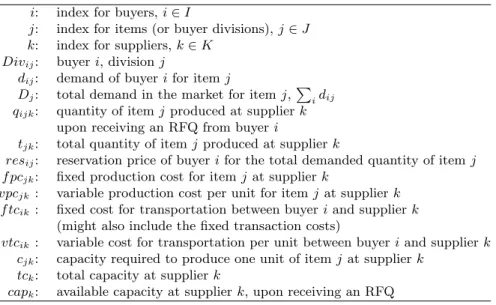
Table 1.1. Glossary of Notation

i: index for buyers,i∈I

j: index for items (or buyer divisions),j∈J k: index for suppliers,k∈K

Divij: buyeri, divisionj

dij: demand of buyerifor itemj

Dj: total demand in the market for itemj,

P

idij

qijk: quantity of itemjproduced at supplierk

upon receiving an RFQ from buyeri

tjk: total quantity of itemjproduced at supplierk

resij: reservation price of buyerifor the total demanded quantity of itemj

f pcjk: fixed production cost for itemjat supplierk

vpcjk: variable production cost per unit for itemjat supplierk

f tcik: fixed cost for transportation between buyeriand supplierk

(might also include the fixed transaction costs)

vtcik: variable cost for transportation per unit between buyeriand supplierk

cjk: capacity required to produce one unit of itemjat supplierk

tck: total capacity at supplierk

capk: available capacity at supplierk, upon receiving an RFQ

3.1.

No Collaboration

In this market structure, we model traditional marketplaces, where neither the functional divisions of a buyer nor different buyers in the market collaborate with each other. As discussed earlier, many firms have uncoordinated purchasing divisions. For example, until recently Chevron’s procurement structure was fragmented and decentralized where “people at many different locations were buying many materials, (often the same materials) from their favorite suppliers, or on an as-needed basis” (Reilly (2001)).

We assume that the functional divisions arrive sequentially and in-dependently to the market. Therefore the marketplace can be thought of as a queue of buyer divisions each with an RFQ for a specific item. When a buyer division makes a contracting decision, she is unaware of the other buyer divisions’ demands or procurement decisions (including the ones both from the same and different companies), or about the cur-rent order status at the suppliers. After submitting an RFQ, a buyer division makes the contracting decision only based on the unit prices quoted by the suppliers. Once the contracting decision is made and the purchase order is submitted by a buyer division, another buyer division arrives to the market and submits an RFQ.

Buyer divisions’ decisions in contracting depend on the kind of infor-mation they receive from the suppliers. A supplier can provide either

a pessimistic or an optimistic quote to a buyer. When providing a pessimistic quote, the supplier regards that buyer as if she will be the last one to contract for that item. When providing an optimistic quote

(opt), the supplier assumes that he will supply all the demand in the

market for that item. The optimistic quote is a lower bound on the final contract price, whereas the pessimistic quote is an upper bound.

Given an RFQ by buyer divisionj of company ifordij units of item

j, the supplier computes the pessimistic quote (bid price per unit) as

follows: bid_ijk= f pcjk qijk+dij +vpc_jk+Pf tcik m∈Sdim +vtc_ik (1.1)

The first two terms in equation (1.1) correspond to the unit production

cost, Pk(dij). The fixed production cost for an item is shared among

multiple buyer divisions (from different companies) who placed orders

for that item with the supplier. q_ijk is the total quantity for item j

already contracted at supplierk upon receiving the RFQ of company i

divisionj.

The last two terms of equation (1.1) correspond to the unit

trans-portation cost, T_k(dij). The fixed transportation cost is shared among

multiple buyer divisions from the same company who placed orders (for

different items) with the same supplier. The set S contains buyer

di-vision j and the other buyer divisions of company i that have already

contracted with supplierk.

Note that if a buyer division is the first one to place an order for an

item at a supplier, then she is quoted all the f pc. Similarly, when a

supplier receives an RFQ for the first time from a buyer division of a

particular company, he incorporates all thef tcin the bid.

To compute the optimistic quote, supplier k needs to first compute

(an upper bound on) the maximum total quantity of orders for item j

he could produce upon receiving an RFQ, which is:

Qijk= min

(

Dj, qijk+cap_c k jk

)

The maximum total quantity is bounded by the minimum of two

terms. The first is the total demand for item j in the market. The

second is the quantity of item j already produced by supplier k plus

the maximum additional quantity of item j that can be produced by

supplierk.

Therefore the following term is a lower bound on the fixed production cost per unit:

max ( f pcjk D_j , f pcjk q_ijk+capk cjk ) .

Upon receiving an RFQ, supplierkcomputes the following optimistic

quote for buyeriper unit of itemj:

optijk= f pc_jk Qijk + f tcik P m∈Sdim +vpcjk+vtcik (1.2)

In the remainder of the paper, we assume that the supplier provides a pessimistic quote unless otherwise stated.

If buyericontracts with supplier k, the final contract price she pays

per unit of itemj is:

priceijk= f pc_t jk jk

+vpcjk+Pf tcik

m∈Sdim+vtcik, (1.3)

wheret_jk is the total quantity of itemj produced at supplierkin the

final matching. The contract price of an item has a similar structure to the bid price for that item. As the number of buyers contracting with a supplier for the same item increases, the unit price to be paid by a buyer decreases. Therefore, in the end the price paid by a buyer might be lower than the quoted price.

The practice of lower final prices paid by the buyers compared to the initial bids offered by the suppliers is commonly observed in group purchasing programs. For example, the price of a product goes down as more buyers join the group and agree to buy that product at the current posted price. Although some buyers may have joined the group (and committed to purchasing) while the price was higher, in the end all the buyers pay the final, lowest price.

In the final matching, the surplus of buyericontracted with supplier

kfor itemj is:

surplusij = (resij−priceijk·dij) (1.4)

Note that when considering the supplier bids the buyer division mul-tiplies the bid price with the total demand for the item to evaluate her surplus.

3.1.1 Buyer Strategies. A buyer division submits RFQs

to the suppliers for the item she demands and chooses a supplier with the goal of maximizing her surplus. We consider the following buyer strategies for accepting or rejecting a bid.

1 If some of the supplier bids are lower than her reservation price, the buyer division accepts the minimum bid.

2 If all the bids are higher than the buyer division’s reservation price,

(a) she accepts the minimum bid with probability α.

(b) she rejects all the bids with probability 1-α, and

i with probability β, she leaves the market permanently.

ii with probability 1−βshe returns to the market (i.e., joins

the end of the queue) since there is a possibility that the minimum bid the buyer receives later is lower than the current minimum bid. The buyer stays in the market until her surplus becomes positive or the bid prices stop decreasing, whichever happens first.

Having defined a general scheme, we consider the following six buyer

strategies resulting from specific choices ofα and β. In each of these, a

buyer division makes a contract with the supplier that offers the mini-mum bid, if that bid is below her reservation price. Otherwise, the buyer division:

Accept the minimum bid, min (α = 1) Contracts with the lowest bid supplier.

Myopic Strategy,myopic (α= 0,β = 1) Leaves the market.

Leave and possibly return later, loq(α= 0,0< β <1) Leaves the

market with probability 0< β <1, returns to the market and joins the

end of the queue with probability 1−β.

Leave and return later, q(α= 0,β = 0) Returns to the market and joins the end of the queue.

Accept the lowest bid or leave and return later,aoq(0< α <1,

β = 0) Accepts the minimum bid with probability α. With probability

1-α she rejects all the bids and joins the end of the queue.

Minimum optimistic bid, mobAccepts the minimum optimistic bid, min_k{opt_ijk}.

Example: Consider a marketplace where there are four buyer divisions,

Divij, i= 1,2, j = 1,2 (two companies with two divisions each), three

responsible for itemIj,j = 1,2. The buyer divisions arrive to the market

in the following order: (1) company 1 division 1, (2) company 2 division 1, (3) company 1 division 2, (4) company 2 division 2. Buyer divisions

use the accept the minimum bid strategy for contracting decisions. For

simplicity we assume that the suppliers are uncapacitated. The

infor-mation regarding buyer divisions (Div), suppliers (S) and items (I) is

listed in the Tables 1.2-1.8.

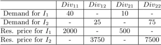
Table 1.2. Demand and reservation prices

Div11 Div12 Div21 Div22

Demand forI1 40 - 10

-Demand forI2 - 25 - 75

Res. price forI1 2000 - 500

-Res. price forI2 - 3750 - 7500

Company 1 division 1 places an RFQ for item 1. The quoted bids per unit of item 1 by supplier 1, supplier 2 and supplier 3 are 18.75, 131.37 and 19.00 respectively (refer to equation (1.1)). Supplier 1 wins the contract for item 1.

Next, company 2 division 1 arrives to the market and submits an RFQ for item 1. Supplier 1 has already initiated production for item 1. Therefore supplier 1 reflects only some portion of the fixed production cost in the quote, whereas supplier 2 and supplier 3 reflect all the fixed production cost in their quotes. The quotes per unit of item 1 by sup-pliers 1, 2 and 3 are 24.00, 486.00 and 30.00 respectively. Company 2 division 1 contracts with supplier 1 for item 1.

Table 1.3. Fixed and variable production costs

S1 S2 S3

I1 f pc11= 100 f pc12= 140 f pc13= 100 vpc11= 10 vpc12= 10 vpc13= 10 I2 f pc21= 9125 f pc22= 100 f pc23= 4605

vpc21= 10 vpc22= 10 vpc23= 10

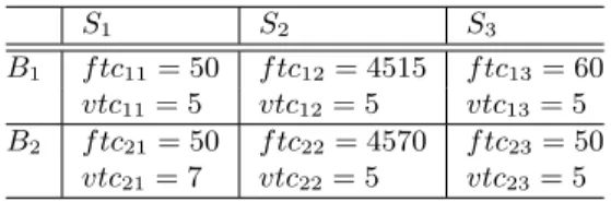
Next, company 1 division 2 places an RFQ for item 2. While quoting the bids, supplier 1 incorporates only some portion of the fixed trans-portation cost, since supplier 1 has already contracted with division 1 of the same company for item 1. The bids quoted by suppliers 1, 2 and 3 are 380.77, 199.60, 201.60, respectively. For item 2, company 1

divi-Table 1.4. Fixed and variable transportation costs S1 S2 S3 B1 f tc11= 50 f tc12= 4515 f tc13= 60 vtc11= 5 vtc12= 5 vtc13= 5 B2 f tc21= 50 f tc22= 4570 f tc23= 50 vtc21= 7 vtc22= 5 vtc23= 5

sion 2 contracts with supplier 2 and is charged for two different fixed transportation costs by both supplier 1 and supplier 2. The surplus she obtains for item 2 isres12−bid122·d12= 3750−199.60·25 =−1240.00. Although the surplus value is negative, since the strategy under

consid-eration isaccept the minimum bid, this does not impose any restriction

on contracting.

Finally company 2, division 2 submits an RFQ for item 2. Supplier 2 has initiated production for item 2. The quotes for item 2 by suppliers 1, 2 and 3 are 139.25, 76.93, 77.07, respectively. For item 2, company 2 division 2 contracts with supplier 2. She is also charged for two different fixed transportation costs. Bid prices and contracted suppliers are shown in Table 1.5.

Table 1.5. Bid Prices

S1 S2 S3

Div11 bid111=18.75 bid112 = 131.75 bid113= 19.00 Div12 bid121= 380.77 bid122=199.60 bid123= 201.60 Div21 bid211=24.00 bid212 = 486.00 bid213= 30.00 Div22 bid221= 139.25 bid222=76.93 bid223= 77.07

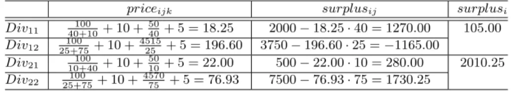
The contract prices paid by the buyers are shown in Table 1.6 and the total surplus is 2115.25. The matching for the no collaboration example is shown in Figure 1.2(a). In the following sections we analyze the same example under different collaboration models.

3.2.

Internal Collaboration

Advances in information technology and enterprise systems have creased the availability of real-time data. This, in turn, has led to in-creased levels of information sharing and collaboration among the di-visions (or business units) of a company. Before 1997, each division of Siemens Medical Systems had its own supplier and this significantly

de-Table 1.6. Contract prices and Surplus

priceijk surplusij surplusi

Div11 ₄₀₊₁₀100 + 10 + 50₄₀+ 5 = 18.25 2000−18.25·40 = 1270.00 105.00 Div12 ₂₅₊₇₅100 + 10 + 4515₂₅ + 5 = 196.60 3750−196.60·25 =−1165.00

Div21 ₁₀₊₄₀100 + 10 + 50₁₀+ 5 = 22.00 500−22.00·10 = 280.00 2010.25 Div22 ₂₅₊₇₅100 + 10 +4570₇₅ + 5 = 76.93 7500−76.93·75 = 1730.25

teriorated buying power. Centralization of purchasing has saved 25% on material costs (Carbone (2001)). Similarly, Chevron Corp. is aiming to cut 5% to 15% from annual expenditures by centralizing the procure-ment system and by leveraging volume buys (Reilly (2001)).

In this section we assume that the procurement function is centralized within each company. Equivalently, multiple divisions within a com-pany collaborate for procurement. We also assume that buyers know

the structure of the transportation cost (f tcand vtc) for each supplier,

possibly specified by a long-term contract. Examples of such practices are commonly found in the procurement of transportation services, such as trucking or sea cargo. Shippers contract with multiple carriers where each contract specifies a volume-based price and capacity availability. However, the buyers usually do not have to commit to a shipment vol-ume in these contracts; even if they do, such minimum volvol-ume com-mitments are typically not enforced by the carriers. In our model, the price structure is defined by fixed and variable costs, i.e., suppliers offer

volume discounts. We assume that a buyer i can request and receive

information about the available total capacity, cap_k, and the

volume-based price quotePk(dij) (first two terms of equation (1.1)) for any item

jfrom a supplierk for her entire demandd_ij. This implies that a buyer

can determine the total cost for an order using the information on the transportation cost component and the quote on the production cost component for any item-supplier combination.

Under internal collaboration each buyer decides how much of each product to procure from each supplier using a centralized mechanism.

The procurement decision of buyer i can be modelled by the following

linear integer program.

xijk: 1, if buyericontracts with supplier k for itemj.

maxX j X k resij·xijk− X j X k (Pk(dij) +vtcik)·dij·xijk− X k f tcik·yik (1.5) subject to _X j cjk·dij ·xijk ≤capk ∀k (1.6) (IP-I) xijk≤yik ∀j, k (1.7) X k x_ijk = 1 ∀j (1.8)

Constraints (1.6) ensure that the amount of demand satisfied by a supplier does not exceed the current available capacity of the supplier. Constraints (1.7) ensure that when a contract is made with a supplier the corresponding fixed transportation cost is charged to the buyer. Con-straints (1.8) ensure that the buyer contracts with a single supplier per item. (Note that a more compact formulation is possible by multiplying

the right hand side of (1.6) byy_ik and removing constraints (1.7).)

The buyers contract with the suppliers sequentially as in the no col-laboration model. Constraints (1.8) imply that even if the buyer surplus is negative after solving IP-I, the buyer still makes the contract. Each buyer makes the contracting decision based on maximizing her current surplus in equation (1.5). In the final matching, the contract price and

the surplus of buyer i for item j is obtained as in equations (1.3) and

(1.4).

Example(cont.): We analyze our previous example assuming that each company makes its procurement decisions centrally. Buyer 1 (both di-visions of company 1) arrives to the market and makes the contracting decisions for both items by solving IP-I. Based on the outcome of the model, buyer 1 contracts with supplier 2 for both items and is charged the fixed transportation cost only once.

When buyer 1 makes her contract, supplier 2 initiates production for both items. Therefore, if buyer 2 also contracts with supplier 2, the associated fixed production cost for both items will be shared among

the two buyers. Buyer 2 solves the same model with updated P2(d21)

and P₂(d₂₂) values. The solution suggests that buyer 2 also contracts

with supplier 2 for both items. Therefore the buyers benefit from both economies of scale and scope.

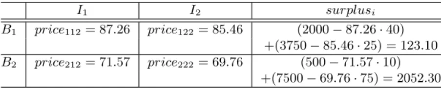
For buyer 1 the final contract price per unit of item 1 is 87.26 and the final price per unit of item 2 is 85.46. Therefore the total surplus of buyer

1 is 123.10. For buyer 2, the contract prices per unit of item 1 and 2 are, 71.57 and 69.76. The total surplus of buyer 2 is 2052.30. As compared to the traditional market, both buyers have increased their total surplus.

The overall buyer surplus obtained in the market is 2175.40.

Table 1.7. Contract prices and surplus

I1 I2 surplusi B1 price112= 87.26 price122= 85.46 (2000−87.26·40) +(3750−85.46·25) = 123.10 B2 price212= 71.57 price222= 69.76 (500−71.57·10) +(7500−69.76·75) = 2052.30

3.3.

Full Collaboration

In the full collaboration model, we assume that a third party interme-diary enables collaboration among multiple buyers. We use the terms e-market and full collaboration interchangeably. However, in practice not all e-markets enable full collaboration. Some e-markets provide only catalog services where suppliers and buyers post supply and de-mand quantities. 3PL providers such as Transplace or C.H. Robinson, where shippers and carriers do not contract directly with each other but through the 3PL intermediary, may enable full collaboration.

In this model, each buyer submits her demand and reservation price for each item, and each supplier submits cost and capacity information to the intermediary. The intermediary in turn matches supply and demand in the market with the objective of maximizing the total buyer surplus. The matching program faced by the intermediary can be modeled by the following linear integer problem, which is a slight modification of (IP-I):

z_jk: 1, if supplierkinitiates production for itemj.

maxX i X j X k res_ij ·x_ijk−X j X k f pc_jk·z_jk−X i X k f tc_ik·y_ik −X i X j X k (vpcjk+vtcik)·dij·xijk (1.9) subject to (1.7) and (1.8) ∀i X i X j cjk·dij ·xijk ≤tck ∀k (1.10)

x_ijk ≤z_jk ∀i, j, k (1.11) Constraint (1.10) ensures that the amount of demand satisfied by a supplier does not exceed the total capacity of the supplier. Constraint (1.11) ensures that when production is initiated at a supplier for an item, a fixed production cost is incurred for that item.

In the final matching, the contract price and surplus of buyer i for

itemj is obtained as in equations (1.3) and (1.4). While matching

sup-ply and demand, it is possible that some buyers have a negative surplus.

Example(cont.): Using our previous example, we illustrate the full col-laboration model where the intermediary simultaneously matches buyers and suppliers. Under this model both companies contract with supplier 3 on both items. The contract prices and the surplus are given in ble 1.8. The total buyer surplus under this model is 6685.00. See Ta-ble 1.9 for a comparison of the surplus obtained by each buyer under three collaboration models.

Table 1.8. Contract prices and surplus

I1 I2 surplusi

B1 price113= 17.92 price123= 61.97 (2000−17.92·40)

+(3750−61.97·25) = 3483.75

B2 price213= 17.58 price223= 61.63 (500−17.58·10)

+(7500−61.63·75) = 3201.25

As seen in Figure 1.2, increasing collaboration levels among buyers leads to different matchings.

In these collaborative environments, the intermediary should well as-sess the implications of antitrust laws. Collaboration in the e-market might give incentives to the participants to collude in the upstream or downstream marketplaces. Therefore intermediaries should keep sensi-tive information such as output levels, reservation prices, costs or ca-pacity levels, confidential. The total surplus obtained under full collab-oration provides an upper bound on the surplus that would be obtained under less collaborative environments. Thus even if full collaboration is not possible due to antitrust laws or other reasons, the upper bound would provide valuable information for the intermediary and the partic-ipants.

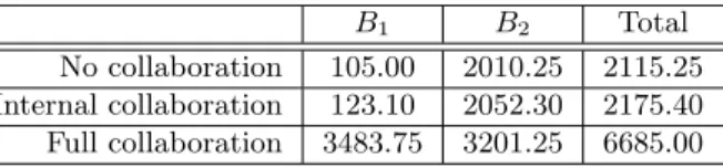
Table 1.9. Surplus obtained by each buyer

B1 B2 Total

No collaboration 105.00 2010.25 2115.25 Internal collaboration 123.10 2052.30 2175.40 Full collaboration 3483.75 3201.25 6685.00

4.

Experimental Design

In this section we test how the three collaboration models perform under different market conditions. We consider a market with 25 buyers, 6 suppliers and 3 items. Each buyer places RFQs for all 3 items and suppliers have the capability to produce any of the items. We assume that the capacity required to produce one unit of any item is 1.

The parameters that define the marketplace are listed in Table 1.10. We selected the following three factors for controlling the market struc-ture:

1 Market supply (total capacity).

2 Manufacturing set-up cost (f pc) versus variable production cost

(vpc).

3 Fixed transportation cost (f tc) versus variable transportation cost

(vtc).

We define two levels (low and high) for each of the three factors and obtain 8 different market settings.

4.1.

Design Parameters

4.1.1 Market Supply vs. Market Demand. The demand of

each buyer for each item is generated from a uniform distribution U[d,d]

(see Table 1.10). The market supply is defined as the total production capacity of the market, which can be either “low” or “high” compared to the expected total demand in the market. We model low (high) market supply by setting the supply equal to the lower (upper) bound of the total demand.

Average total capacity required to satisfy low market demand =

T C_low= (# of buyers)·(# of items per buyer)·(dper item)

·(avg. capacity required per unit)

Average total capacity required to satisfy high market demand =

T C_high= (# of buyers)·(# of items per buyer)·( ¯dper item)

·(avg. capacity required per unit)

In our experiments we assume that the capacities of the suppliers are equal and hence the capacity per supplier is the total market capacity divided by the number of suppliers.

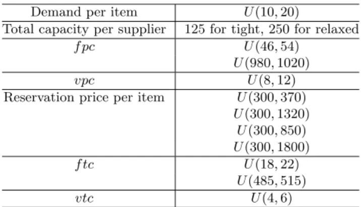
Table 1.10. The parameters of the market

Demand per item U(10,20)

Total capacity per supplier 125 for tight, 250 for relaxed

f pc U(46,54)

U(980,1020)

vpc U(8,12) Reservation price per item U(300,370)

U(300,1320) U(300,850) U(300,1800) f tc U(18,22) U(485,515) vtc U(4,6)

4.1.2 Fixed Costs of Manufacturing and Transportation.

The average setup cost of production, i.e., the mean of f pc, is set

at either “low” or “high” levels as compared to the average variable

are generated randomly from the uniform distributions U[46,54] and

U[980,1020], for the low and highf pclevels, respectively.

The fixed cost of transportation,f tc, is set either at “low” or “high”

levels as compared tovtc, whereµf tc=20 or 500 andµvtc=5. f tcvalues

are generated randomly from the uniform distributions U[18,22] and U[485,515], for the low and high cases, respectively.

Note that rather than the individual values off pc,f tc,vpcandvtc, we consider the ratios f pc_vpc and f tc_vtc as the design factors in our experiments.

4.1.3 Reservation Price. We generate the reservation prices

of the buyers randomly from the uniform distributionU ∼[(vpc+vtc)·

d, f pc+f tc+ (vpc+vtc)·d]. The lower bound corresponds to the case where (in the limit) the buyer only pays the variable costs. The upper bound corresponds to the worst case where a buyer incurs the entire fixed production and transportation cost, in addition to the variable costs. Table 1.11. Upper and lower bound for reservation price in four different market types

Market type µf pc,µf tc Reservation price

1 (50,20) U(300,370) 2 (1000,20) U(300,1320) 3 (50,500) U(300,850) 4 (1000,500) U(300,1800)

The design factors and factor levels are shown in Table 1.12. Table 1.12. Design factors and factor levels

Levels low high Factor 1 Supply/Demand .66 1.33 Factor 2 f pc/vpc 5 100 Factor 3 f tc/vtc 4 10

4.2.

Buyer strategies

In our experiments, we consider the following buyer strategies defined previously:

(a) Myopic strategy (myopic)

(b) Accept the minimum bid (min)

(c) Leave and possibly return later (loq) withβ = D

Q

(d) Leave and return later (q)

(e) Accept the lowest bid or leave and return later (aoq) with

α= 0.25

(f) Minimum optimistic bid (mob)

2 Internal collaboration (int)

3 Full collaboration (e-market)

4.3.

Performance Measures

To evaluate the effectiveness of different bidding strategies under vari-ous market conditions, we consider the following performance measures:

1 % of satisfied demand = quantity of satisfied demand_{total market demand} ·100 2 total surplus = total reservation price - total cost

3 average surplus per unit= _{quantity of satisfied demand}total surplus 4 average cost per unit= _{quantity of satisfied demand}total cost

From a buyer’s perspective, it is desirable to have a high amount of sat-isfied demand (market liquidity), and a high surplus per unit of satsat-isfied demand (quality of surplus), leading to a high total buyer surplus. Note that the quality of surplus is inversely proportional to the suppliers’ costs per unit, i.e., a strategy which decreases the setup effort in the market is desirable.

Current e-marketplaces focus on similar performance measures. For example, Transplace uses the capacity of several carriers to satisfy de-mand, which makes it an attractive choice for shippers in terms of demand satisfaction. Similarly, consortia e-marketplaces such as Cov-isint.com help buyers to achieve economies of scale and therefore reduce average cost per unit.

5.

Experimental Results

In this section we compare the strategies with respect to the perfor-mance measures. Each market consists of 25 buyers, 6 suppliers, and 3 items. The results are obtained and compared using a t-test for 8 market

types and 8 strategies, with 15 runs for each market type and strategy combination.

The market types are indicated by a 3 digit codeabc, wherea,b,c∈{0,1}.

0 corresponds to low level setting for that factor and 1 corresponds to

highlevel. aindicates capacity level in the market, bindicates f pc_vpc level

and c indicates f tc_vtc level. For example, the 101 market corresponds to

high capacity, low fixed cost of production and high fixed cost of trans-portation.

The results are presented in Tables 1.13-1.19. In Tables 1.14, 1.16,

1.18 and 1.20 a “>” sign indicates that a strategy has resulted in a

higher value at the indicated significance level (SL). If two strategies are in the same set, then their performances are not significantly different from each other.

5.1.

Results for the percentage of satisfied

demand

Observation 1 In maximizing the percentage of satisfied demand, when capacity is high

i. aoq,min,moband intperform best, followed by e-market, followed by q, followed by loq and myopic.

ii. If there are no economies of scale and scope (market 100), then

loqand myopichave similar performance; otherwise,loqoutperforms

myopic.

It is not surprising thatmob,min and intperform well in satisfying

the demand since they do not consider reservation prices. Sinceaoq

ac-cepts offers with some probability even if they are above the reservation price, it also performs well in satisfying the demand.

Observation 2 In maximizing the percentage of satisfied demand, when capacity is low

i. e-market is at least as good as any other strategy.

ii. When benefits from economies of scale or scope are high myopic and

loq are always the worst, followed by q.

iii. min, int, aoq and mob have similar performance when there are economies of scope. When there are no economies of scope, e-market

dominates other strategies.

Note that myopic and loq are always the worst in satisfying the

demand except for 000, followed byq, regardless of the capacity level in

Table 1.13. Satisfied demand in different markets (all figures are percentages) Market type myopic min q aoq loq mob int e-market

000 65.0 65.0 65.0 64.8 65.0 64.3 64.8 65.5 001 21.2 64.5 27.2 64.8 21.2 64.5 64.8 64.9 010 29.8 64.9 35.9 65.0 29.8 63.9 64.6 65.4 011 19.9 64.5 26.6 64.5 19.9 64.5 64.6 65.1 100 95.1 100.0 97.4 100.0 95.5 100.0 100.0 99.4 101 22.2 100.0 35.4 99.8 25.0 100.0 100.0 94.7 110 40.9 100.0 57.1 100.0 46.7 100.0 100.0 96.3 111 26.0 100.0 42.7 99.8 30.2 100.0 100.0 84.7

Table 1.14. Comparison of strategies with respect to the percentage of satisfied de-mand

Market

type Performance sl

000 e-market>{min,myopic=loq=q,aoq,int,mob} 97% 001 {e-market,int,aoq,min,mob}>q>{myopic=loq} 99% 010 e-market>{aoq,min}>int>mob>q>{myopic=loq} 96% 011 {e-market,int,min,mob,aoq}>q>{myopic=loq} 99% 100 {aoq=min=mob=int}>e-market>q>{loq,myopic} 99% 101 {min=mob=int,aoq,}>e-market>q>loq>myopic 99% 110 {aoq=min=mob=int}>e-market>q>loq>myopic 99% 111 {min=mob=int,aoq,}>e-market>q>loq>myopic 99%

5.2.

Results for total surplus

Observation 3 e-market outperforms all other strategies in terms of total surplus under any market structure. The benefit of e-market com-pared to the next best strategy is highest when the capacity is low and there are economies of scale and scope (Figure 1.3).

Observation 4 In maximizing the total surplus

i. int outperforms mob when there are economies of scope (markets 001, 011, 101 and 111).

ii. minoutperforms intwhen there are economies of scale but not scope (markets 010 and 110).

iii. qoutperforms loqwhen there are either economies of scale or scope or when the capacity is high. In market 000, q and loq have the same performance.

iv. mob outperforms or does as well as min in all markets. The dif-ference between mob and min is greatest when the capacity is high and there are only economies of scope (market 101).

v. aoq outperforms loq when there are economies of scale (markets 010, 011, 110, 111); otherwise loq either outperforms or does as well as aoq.

Observation 4.i is in line with the fact that int tries to consolidate

orders of the same buyer for different products and therefore saves on

transportation cost, whereas mob focuses on lowering the production

cost by consolidating orders from different buyers for the same product.

Observation 4.ii implies that when the benefits from economies of

scale are high, themin strategy leads to fewer production initiations as

compared to theintstrategy. In theintstrategy, due to collaboration,

the buyer divisions arrive to the system at the same time and contract with a set of suppliers to maximize their overall surplus. Although the fixed cost of transportation is low, experimental results indicate that it is still more beneficial for a buyer to contract with fewer suppliers than the number of items she demands. Please note that this may not

be the case if the variance ofvariable transportation cost is sufficiently

high. In that case a buyer could select a different supplier for each of

her items. In the min strategy, buyer divisions arrive to the market

independently. For most of the cases two divisions of the same buyer are not assigned to the same supplier because they arrive at different times and the same supplier is no longer available for the division that arrives later. Therefore in most of the instances a supplier uses all of his

capacity to produce a single item, whereas in theintstrategy a supplier

each buyer contracting with a supplier for two or more items causes

more suppliers to initiate production as compared to themin strategy.

As a result, while losses from economies of scale are high, gains from

economies of scope are insignificant in theintstrategy.

Observation 4.iv indicates that the “lookahead” policy employed by

the mob strategy helps to increase the surplus compared to the min

strategy, which does not consider potential future arrivals.

Observa-tions 4.iiiand 4.vshow that the total surplus can increase if the buyers

accept the lowest bid even if it is above their reservation price, or return to the market with a positive probability.

We should note that the observations may partly depend on the

ex-perimental settings. For instance, observation 4.ii might change if the

cost values assigned to each supplier had much smaller variance. In that

case, theintstrategy would not necessarily lead to more production

ini-tiations and buyer-supplier assignments would have a similar structure

to theminstrategy.

In our experimental design we limited the number of items that each buyer is willing to buy to three, due to computational difficulties.

How-ever we conjecture that as the number of items increases, int strategy

will achieve a higher total surplus in the presence of economies of scope.

When only economies of scale exist, int strategy might perform worse

due to observation 4.ii.

Table 1.15. Total surplus in different markets (all figures are in thousands).

Market

type myopic min q aoq loq mob int e-mkt

000 5.031 4.629 5.032 4.940 4.503 4.530 4.588 6.703 001 3.220 −3.495 4.614 −3.142 3.220 −1.850 6.046 10.706 010 13.404 16.744 16.176 21.444 13.404 18.245 13.681 29.635 011 8.418 5.064 11.217 12.826 8.418 6.653 10.108 24.932 100 7.607 7.617 7.647 7.626 7.611 7.612 7.750 8.318 101 3.557 7.002 6.671 3.693 4.343 5.970 12.555 13.078 110 18.201 33.263 24.332 33.655 20.330 34.265 31.781 35.950 111 11.724 16.597 18.110 16.768 13.367 20.300 30.563 33.502

5.3.

Results for average surplus per unit

Observation 5 In maximizing the average surplus, when the capacity is low

Table 1.16. Comparison of the strategies with respect to total surplus in different markets

Market

type Performance sl

000 e-market>{myopic=loq=q}>aoq>{min,int,mob} 99% 001 e-market>int>q>{myopic=loq}>aoq>mob>min 99% 010 e-market>aoq>mob>{min,q}>{int,myopic=loq} 95% 011 e-market>aoq>{q,int}>{myopic=loq}>mob>min 90% 100 e-market>int>q>{aoq,min,mob,loq,myopic} 90% 101 e-market>int>{q,mob}>{loq,aoq,myopic}>min 98% 110 e-market>{mob,aoq,min}>int>q>loq>myopic 99% 111 e-market>int>{mob,aoq,q,min}>{loq,myopic} 99%

Figure 1.3. % difference in the total surplus between e-market and the next best strategy under different market types

i. e-market outperforms or does at least as well as any other strategy. ii. aoq outperforms mob and min.

Observation 6 In maximizing the average surplus,

i. myopic, q and loq perform at least as well as or better than all strategies except e-market.

ii. min has the worst performance except when there are only economies of scale (markets 010 and 110), in which case int performs worst.

Note that the strategies which consider reservation prices (myopic,

loq or q) result in higher average surplus compared to the strategies

which do not. Recall that these strategies do not perform well in satis-fying the demand (Observation 1). On the other hand, strategies which

do not consider reservation prices (min and mob) result in lower

aver-age surplus levels, but higher percentaver-ages of satisfied demand. In these strategies it is possible that some buyers obtain a negative surplus. These results imply a significant trade-off between high satisfied demand and the average surplus.

Under tight capacity Observation 4.i also holds for maximizing the

average surplus, i.e.,mob does better when there is economies of scale

andint does better when there are economies of scope.

Table 1.17. Average surplus per unit in different markets Market

type myopic min q aoq loq mob int e-market

000 6.9 6.3 6.9 6.8 6.9 6.3 6.3 9.1 001 13.5 −4.8 15.3 −0.4 13.5 −2.5 8.3 14.7 010 40.1 22.9 40.3 29.3 40.1 25.4 18.9 40.3 011 37.3 7.0 37.5 17.7 37.3 9.2 13.9 34.1 100 7.1 6.8 7.0 6.8 7.1 6.8 6.9 7.5 101 14.1 0.6 16.8 3.0 15.4 5.3 11.2 12.3 110 39.5 29.6 38.3 29.9 38.7 30.5 28.3 33.3 111 40.2 14.8 38.5 15.0 39.5 18.1 27.2 35.4

5.4.

Results for average cost per unit

Observation 7 e-market always has the lowest average cost, except when the capacity is high and there are only economies of scale (market 110).

Table 1.18. Comparison of the strategies with respect to average surplus in different markets

Market

type Performance sl

000 e-market>{myopic=loq=q}>aoq>{min,int,mob} 99% 001 {q, e-market}>{myopic=loq}>int>aoq>mob>min 88% 010 {e-market,q,myopic=loq}>aoq>mob>min>int 99% 011 {q,myopic=loq,e-market}>aoq>int>mob>min 99% 100 e-market>myopic>loq>{q,int}>{aoq,min,mob} 90% 101 q>loq>myopic>e-market>int>mob>aoq>min 95% 110 myopic>{loq,q}>e-market>{mob,aoq,min}>int 95% 111 {myopic,loq,q}>e-market>int>mob>{aoq,min} 93%

Observation 8 min has the highest average cost except when there are only economies of scale (markets 010 and 110), in which case int has the highest average cost.

It is interesting to note that when int is not the worst performer

in average cost, it is the second best. This leads us to conclude that collaboration helps to decrease the average cost per unit, especially when

economies of scale and scope are high. In comparing mob and int,

Observation 4.i also holds for minimizing the average cost, i.e., mob

does better when there are economies of scale andintdoes better when

there are economies of scope.

Table 1.19. Average cost per unit in different markets Market

type myopic min q aoq loq mob int e-market

000 16.0 16.2 16.0 16.0 16.0 16.2 16.0 15.4 001 40.8 42.6 36.5 41.3 40.8 40.5 29.4 28.3 010 26.8 29.8 24.7 28.7 26.8 27.5 34.0 23.7 011 62.7 61.6 58.8 60.8 62.7 59.6 54.4 50.4 100 15.4 15.5 15.4 15.4 15.4 15.4 15.3 14.8 101 39.8 37.0 32.3 34.3 37.1 32.3 26.4 25.0 110 22.5 23.0 20.1 22.7 21.2 22.1 24.3 21.1 111 57.0 53.1 52.1 53.0 55.2 49.9 40.7 39.6

Before closing this section, we would like to briefly discuss how our assumptions of “the buyers being located in the same region” and “each buyer division being responsible for the procurement of one item”

af-Table 1.20. Comparison of the strategies with respect to average cost in different markets

Market

type Performance sl

000 {mob,min}>{aoq,q=myopic=loq,int}>e-market 99% 001 min>{aoq,myopic=loq,mob}>q>int>e-market 99% 010 int>{min,aoq}>{mob,myopic=loq}>q>e-market 95% 011 {myopic=loq,min,aoq}>{mob,q}>int>e-market 95% 100 {mob,min,aoq,q,loq,myopic,int}>e-market 99% 101 myopic>{loq,min}>aoq>{q,mob}>{int,e-market} 98% 110 int>{min,aoq,myopic,mob}>{loq,e-market}>q 80% 111 myopic>loq>{min,aoq,q}>mob>int>e-market 97%

fect the experimental results. If these two assumptions were to be re-laxed, then the structure of the model and the form of collaboration would change. In this case divisions that belong to different buyers located in the same region could achieve savings from transportation, whereas buyer divisions of the same buyer located at different regions could achieve savings from production by leveraging their purchasing power. This might lead to a conclusion that internal collaboration is beneficial when benefits from economies of scale are high. However, full collaboration would still be most beneficial when savings both from economies of scale and scope are high.

6.

Conclusion and Future Work

We analyzed markets where multi-unit transactions over multiple items take place. We considered three different trading models with increasing levels of collaboration among buyers. The “no collaboration” model con-siders traditional markets where there is no collaboration among buyers or buyer divisions. In the “internal collaboration” model, purchasing divisions of a buyer collaborate for procurement. In the “full collab-oration” model an intermediary enables collaboration among different buyers.

We studied six different buyer strategies for the no collaboration model, and one for the internal collaboration model. These strategies were tested against the centralized buyer-seller matching mechanism em-ployed by the intermediary in the “full collaboration” model.

The experimental results show that when there is tight capacity in the market and when potential economies of scope are high (i.e., when the fixed cost of transportation is high), the “full collaboration” model

results in significantly higher total surplus than the other strategies. The increase in surplus is even more pronounced when economies of scale are also high (i.e., when the fixed costs of both manufacturing and trans-portation are high). The extra benefits obtained by full collaboration are relatively low when the capacity is high and the fixed cost factors are low.

We also observe that internal collaboration performs very well, pro-vided that the potential benefits from economies of scope are high. On the other hand, when the potential benefits from economies of scale are high, buyer strategies with a “look-ahead” perform well. These are the strategies which consider potential future trades in the market by other buyers while contracting with a supplier.

Our analysis indicates that the potential benefits of intermediaries are highest in capacitated markets with high fixed production and/or transportation costs. Process industries such as rubber, plastic, steel and paper are typically characterized by high fixed production costs. High fixed transportation costs can arise in industries that have to either manage their own distribution fleet or establish contracts with carriers that guarantee a minimum capacity in order to ensure adequate service levels (e.g., Ford Customer Service Division guarantees routed deliveries to their dealers every three days and hence has high fixed transportation costs. Due to variability in the demand that they face, it can be the case that there is fairly low capacity utilization).

It is important to note that different collaboration models require different coordination, personnel, and technology costs. Although our current models do not account for any fixed or variable costs of imple-menting a collaboration strategy, they could easily be modified to incor-porate such information. Clearly, the benefits should outweigh the costs of implementing a particular strategy for that strategy to be attractive for a firm.

In our future work we are planning to extend the experimental anal-ysis to a larger market size in an effort to observe the effect of market liquidity on performance. In addition, we would like to design allocation mechanisms that are both computationally efficient and perform well across a broad range of performance measures. Finally, it would be in-teresting to consider the issue of pricing strategies for the intermediary such as charging a subscription fee to buyers and/or suppliers versus charging the participants for each transaction.

Aviv, Y.2001. The Effect of Collaborative Forecasting on Supply Chain

Performance. Management Science,47, 1326–1343.

Cachon, G. P. 2003. Supply Chain Coordination with Contracts, S. Graves, T. de Kok, eds., Supply Chain Management-Handbook in OR/MS (forthcoming). North-Holland, Amsterdam.

Cachon, G. P. and Zipkin, P. H. 1999. Competitive and

Coopera-tive Inventory policies in a Two-Stage Supply Chain. Management

Science,45, 936–953.

Carbone, J.2001. Strategic Purchasing Cuts Costs 25% at Siemens. Purchasing, September 20, 29–34.

Cetinkaya, S. and Lee, C. Y.2000. Stock Replenishment and

Ship-ment Scheduling for Vendor-Managed Inventory Systems.

Manage-ment Science,46, 217–232.

Cheung, K. L. and Lee, H. L.2002. The Inventory Benefit of

Ship-ment Coordination and Stock Rebalancing in a Supply Chain.

Man-agement Science,48, 300–306.

Elmaghraby, W. and Keskinocak, P.2002. Ownership in Digital

Marketplaces. European American Business Journal, 71–74.

Gurnani, H.2001. A Study of Quantity discount Pricing Models with Different Ordering Structures: Order Coordination, Order

Consol-idation, and Multi-Tier Ordering Hierarchy. International Journal

of Production Economics,72, 203–225.

Jin, M. and Wu, D. 2001. Supply Chain Contracting in Electronic Markets: Auction and Contracting Mechanisms. Working Paper, Lehigh University, Bethlehem, PA.

Kalagnanam, J., Davenport, A. J. and Lee, H. S. 2001. Com-putational Aspects of Clearing Continuous Call Double Auctions

with Assignment Constraints and Indivisible Demand. Electronic

Commerce Research,1, 221–238.

Keenan, F. and Ante, S. E. 2002. The New Teamwork. Business Week e.biz, February 18, 12–16.

Keskinocak, P. and Tayur, S. 2001. Quantitative Analysis for

Internet-Enabled Supply Chains. Interfaces,31, 70–89.

Ledyard, J. O., Banks, J. S. and Porter, D. P. 1989.

Alloca-tion of Unresponsive and Uncertain Resources. RAND Journal of

Economics,20, 1–25.

Lee, H. L., Padmanbhan, V., Taylor, T. A. and Whang, S.2000.

Price Protection in the Personal Computer Industry. Management

Reilly, C.2001. Chevron Restructures to Leverage Its Buying Volumes. Purchasing, August 9.

Reilly, C. 2002. Specialists Leverage Surfactants, Plastics, Indirect

and Other Products. Purchasing, January 15.

Smyrlis, L. 2000. Secrets of a Successful Marriage: 3PL Users Want a Deeper, more Meaningful Relationship with their 3PL Service

Providers. Are 3PLs ready to commit? Canadian Transportation

Logistics, February.

Stackpole, B.2001. Software Leaders - Trading Exchange Platforms. Managing Automation, June.

Strozniak, P. 2001. Sharing the Load. IndustryWeek, September 1, 47–51.

Weng, Z. K. 1995. Channel Coordination and Quantity Discounts. Management Science,41, 1509–1522.