ON THE DISCOUNTED PENALTY FUNCTION IN A
MARKOV-DEPENDENT RISK MODEL∗
Hansj¨org Albrecher a, b,† Onno J. Boxmac
a Graz University of Technology, Steyrergasse 30, A-8010 Graz, Austria bUniversity of Aarhus, Ny Munkegade, DK-8000 Aarhus C, Denmark
cEindhoven University of Technology and EURANDOM, P.O. Box 513, 5600 MB Eindhoven, The Netherlands
Abstract
We present a unified approach to the analysis of several popular models in collective risk theory. Based on the analysis of the discounted penalty function in a semi-Markovian risk model by means of Laplace-Stieltjes transforms, we rederive and extend some recent results in the field. In particular, the classical compound Poisson model, Sparre Andersen models with phase-type interclaim times and models with causal dependence of a certain Markovian type between claim sizes and interclaim times are contained as special cases.
Keywords: Dependence; classical risk model; Sparre Andersen model; time of ruin; deficit at ruin; surplus before ruin
1
Introduction
Let us consider the following risk model for the surplus processR(t) of an insurance portfolio: R(t) =x+ct− N(t) X j=1 Xj, (1)
where x is the initial capital, c is the premium density which is assumed to be constant, Xj is the size of the jth claim and N(t) is the number of claims up to time t. In classical risk theory, the claims Xj and the claim number process N(t) are assumed to be independent. However, in many applications the independence assumption is too restrictive and recently several authors looked at more general models where this assumption is relaxed in some way (see Asmussen (2000) for a survey on the subject).
∗JEL Classification: G22, Subject and Insurance Branch Code: IM13, Date: June 16, 2005 †Corresponding author. Email: [email protected]; Supported by Fellowship F/04/009 of
In this paper we will consider a semi-Markovian dependence structure of the follow-ing type: Let Wi denote the time between the arrival of the (i−1)th and the ith claim and W0 =X0 = 0 a.s. Then
P(Wn+1 ≤x, Xn+1 ≤y, Zn+1=j|Zn =i,(Wr, Xr, Zr),0≤r≤n)
=P(W1 ≤x, X1 ≤y, Z1=j|Z0 =i) = (1−e−λix)p
ijBj(y), (2) where {Zn, n ≥ 0} is an irreducible discrete-time Markov chain with state space
{1, . . . , M}and transition matrixP = ((pij),1≤i, j ≤M). Thus at each instant of a claim, the Markov chain jumps to a state j, and the distribution Bj of the claim depends on the new state j. Then the next interarrival time is exponentially dis-tributed with parameterλj. Note that given the statesZn−1 andZn, the quantities
Wn and Xn are independent, but there is autocorrelation among consecutive claim sizes and among consecutive interclaim times as well as cross-correlation between
WnandXn. This semi-Markov process was first considered in Janssen and Reinhard (1985), where a formal solution for the survival probabilities in terms of an infinite series of matrix convolutions was derived.
We considerably generalize the approach in Janssen and Reinhard (1985) and inves-tigate the discounted penalty function in such a risk model by means of Laplace-Stieltjes transforms (LST). This allows us to obtain information on several charac-teristics of the risk process.
The model considered in this paper is quite general: it contains the compound Poisson model (M = 1) and Sparre Andersen models with (generalized) Erlang(n)-interclaim distributions (see e.g. Gerber and Shiu (2005), Li and Garrido (2004)) as well as phase-type interclaim distributions (see Avram and Usabel (2004) and Li and Garrido (2005)) as special cases (just choose appropriate transition probabilities and let Bj be degenerate at 0 for all but one state among{1, . . . , M}). Moreover, it also covers models with causal dependence structures of the type considered in Albrecher and Boxma (2004), namely that the distribution of the inter-arrival time depends on the size of the previous claim in a specified way. To see this, choose a generic claim size random variableX and for alli= 1, . . . , M,pij =P(X ∈Aj) for some (possibly random) interval Aj ⊂R and Bj ∼X|X ∈ Aj (cf. Section 6.3). Note that by con-sidering state-dependent transition probabilities pij = P(X ∈ Aj|current state i), we here arrive at a more general model that also allows the claim size distribution itself to depend on the state of the Markov chain. The purpose of this paper can also be seen as to provide an umbrella to the analysis of all these risk models. A fluid queue approach for the Laplace transform of the time until ruin (which is a special case of the discounted penalty function) in a related model can be found in Badescu et al. (2005). For an analysis of the time until ruin based on the methodology of piece-wise deterministic Markov processes, see Jacobsen (2003). For a study on the asymptotic behavior of the ruin function in the presence of depen-dence between interclaim times and claim sizes based on random walk techniques, see Albrecher and Teugels (2004). Adan and Kulkarni (2003) recently considered a
queueing model with dependence structure (2) with λi replaced by λj. Translated to a risk model setting, the latter means that an interclaim time of statej is always followed by a claim size of state (and thus distribution) j (whereas in model (2) it is the other way round). In principle, a similar analysis can be developed for this model, too. However, in view of applications, (2) seems more appealing.
The paper is organized as follows. In Section 2, an explicit expression for the Laplace transform of the discounted penalty function in model (2) is derived. Section 3 then gives an explicit formula for the discounted penalty function for zero initial capital. In Section 4, the asymptotic behavior of the penalty function is investigated for light-tailed claim sizes. In concrete cases, it is sometimes not possible to explicitly evaluate the occurring expressions. Thus, in Section 5 it is shown how to (at least) obtain arbitrary moments of the time to ruin, surplus before ruin and the deficit at ruin. Finally, in Section 6, we specify examples and use the results of the paper to rederive and extend various formulas from the risk theory literature.
2
An equation for the discounted penalty
func-tion
Let µ(ij) denote the jth moment of distribution Bi, given it exists and furthermore
µi :=µ (1)
i . In the sequel we will always assume the net profit condition M X i=1 πiµi < c M X i=1 πiλ−i 1, (3)
whereπ= (π1, . . . , πM) is the stationary distribution of{Zn}. We are now interested in various characteristics of the risk model (1) together with (2). Gerber and Shiu (1998) introduced the by now classical discounted penalty function at ruin
mδ(x) :=E
w(R(Tx−),|R(Tx)|)e−δTx1{Tx<∞}
, (4)
where Tx denotes the time of ruin with initial capital x, R(Tx−) is the surplus im-mediately before ruin, |R(Tx)| is the deficit at ruin and the penalty w(x1, x2) is an arbitrary non-negative function on [0,∞)×[0,∞). δ ≥ 0 may be interpreted as a force of interest, but (4) may also be considered in terms of a Laplace transform with δ as its argument. The function mδ(x) contains a lot of useful information about the risk process. For example, if w ≡ 1, then mδ(x) is the LST of the time to ruin given it occurs, and m0(x) is then simply the ruin probability ψ(x). For
w(x1, x2) = 1{x1≤y1}1{x2≤y2}, m0(x) is just the joint distribution of the surplus be-fore ruin and the deficit at ruin.
We will now derive an integro-differential equation formδ(x) for our Markov additive risk process. Let mδ,i(x) denote the discounted penalty function given thatZ0 =i.
Then by conditioning on the time interval (0, dt), we obtain mδ,i(x) = (1−λidt)e−δdtmδ,i(x+c dt)+λidt M X j=1 pij x+c dt Z 0 e−δdtmδ,j(x+c dt−y)dBj(y) +λidt M X j=1 pij ∞ Z x+c dt e−δdtw(x+c dt, y−x−c dt)dBj(y) +o(dt) (i= 1, . . . , M).
Taylor expansion and rearranging yields
cdmδ,i dx (x)−(λi+δ)mδ,i(x) +λi M X j=1 pij x Z 0 mδ,j(x−y)dBj(y) +λi M X j=1 pij ∞ Z x w(x, y−x)dBj(y) = 0 (i= 1, . . . , M). (5)
Define, for Res ≥0 the Laplace(-Stieltjes) transforms ˜ mδ,i(s) := Z ∞ 0 e−sxmδ,i(x)dx, ˜bi(s) := Z ∞ x=0 e−sxdBi(x), (i= 1, . . . , M), ˜ ωi(s) := Z ∞ x=0 e−sx Z ∞ x w(x, y−x)dBi(y)dx, (i= 1, . . . , M).
Then we obtain for i= 1, . . . , M,
csm˜δ,i(s)−cmδ,i(0)−(λi+δ) ˜mδ,i(s) +λi M X j=1 pij( ˜mδ,j(s)˜bj(s) + ˜ωj(s)) = 0, (6) or in matrix notation, (cs−δ)I−Λ + ΛP B˜(s)m~˜δ(s) =c ~mδ(0)−ΛP ~ω˜(s), (7) whereI is the identity matrix, Λ = diag(λ1, . . . , λM), ˜B(s) = diag(˜b1(s), . . . ,˜bM(s)) and m~˜δ(s) = ( ˜mδ,1(s), . . . ,m˜δ,M(s)).
Thus it remains to solve a system of linear equations. First, the quantities mδ,i(0) have to be determined. For that purpose, denote
Aδ(s) := (cs−δ)I−Λ + ΛPB˜(s).
Proposition 2.1. (i) The equation det(A0(s)) = 0 has one zero s1 = 0 and M −1
zeroes s2, . . . , sM with Re(si)>0.
Proof: Case (i): If δ = 0, then the statement immediately follows from Theorem 3.2 of Adan and Kulkarni (2003) (after transposing their matrix).
Case (ii): We follow an idea in De Smit (1983), see also Adan and Kulkarni (2003). Let C denote a circle with its center at [δ + max1≤i≤Mλi]/c and radius [δ+ max1≤i≤Mλi]/c, and let Aδ(s, u) := (cs−δ)I −Λ +uΛPB˜(s), 0≤ u ≤1. We first prove, for 0≤u≤1, that
det(Aδ(s, u))6= 0 for s∈C. (8) The matrix Aδ(s, u) is diagonally dominant for 0≤u≤ 1, since
|cs−δ−λi+uλipi,i˜bi(s)| ≥ |δ+λi−cs| − |uλipi,i˜bi(s)|
≥ δ+λi−uλipi,i˜bi(0)> uλi(1−pi,i˜bi(0)) = uλi X j6=i pi,j˜bj(0)≥ |uλi X j6=i pi,j˜bj(s)|. (9)
The diagonal dominance implies (cf. Marcus and Minc (1964, pp.146-147)) that detAδ(s, u)6= 0 for s∈C.
Now let f(u) denote the number of zeroes of det(Aδ(s, u)) in C+, the interior of C. Then f(u) = 1 2πi Z C d dsdet(Aδ(s, u)) det(Aδ(s, u)) ds.
Hencef(u) is a continuous function on [0,1], integer valued, and therefore constant.
f(0) = M, because det(A0(s)) = det((cs−δ)I −Λ) = 0 fors∗i := δ+cλi, 1≤i ≤M.
Hence alsof(1) =M. 2
Remark 2.1. It follows from the above proof for Case (ii), and from Remark 6.2 of Adan and Kulkarni (2003) for Case (i), that the zeroes are located in the interior
C+ (s
1 = 0 is located on C in Case (i)).
Remark 2.2. The solutions of
det(Aδ(s)) = 0 (10)
are intimately connected with the behavior ofmδ(x): zeroes with negative real part determine the asymptotic behavior, whereas zeroes in the right half-plane determine the constants in the exact expressions formδ(x). Since for M = 1, this equation is known as the Lundberg fundamental equation (see e.g. Gerber and Shiu (2005)), we call (10) thegeneralized Lundberg fundamental equation.
Now, under the assumption that the functionsmδ,i(x) do not grow super-exponentially fast (which is fulfilled for all penalty functions of practical interest), ˜mδ,i(s) are an-alytic functions for Re(s) ≥ 0, so that for each of the M zeroes s1, . . . , sM we can proceed in the following way: Determine a non-trivial solution~ki of
AT
for each i= 1, . . . , M. Since we then have
0 =m~˜δ(si)T ATδ(si)~ki = (c ~mδ(0)−ΛP ~ω˜(si))T~ki, (11) this gives M linear equations formδ,1(0), . . . , mδ,M(0).
Remark 2.3. For δ = 0, the zeroes s1, . . . , sM can always be obtained numerically. Moreover, if the involved claim size distributions have a rational Laplace transform, then the discounted penalty function can be obtained explicitly by inversion of the Laplace transform of the solution of (7).
3
Zero initial capital
The following explicit expression for the discounted penalty function with zero initial capital can be obtained:
Proposition 3.1. Let K := (~k1, . . . , ~kM)T and let detKj2,i denote the minor of K
with respect to rowj2 and column i. Then
mδ,i(0) = M X j1=1 M X j2=1 Cj(1i),j2(s1, . . . , sM, δ) ˜ωj1(sj2), (i= 1, . . . , M) (12)
where the coefficients Cj(1i),j2(j1, j2 = 1, . . . , M) are given by
Cj(1i),j2 = (−1) i+j2 ·detK j2,i· PM l=1λlpl,j1kj2,l c detK (13)
with kj2,l denoting the l-th component of vector~kj2 (l=1,. . . ,M). Proof: Equations (11) can be written as
c K ~mδ(0) = PM j1=1d (1) j1 ω˜j1(s1) ... PM j1=1d (M) j1 ω˜j1(sM) , with d(jj12) = PM
l=1λlpl,j1kj2,l. An application of Cram´er’s rule gives
mδ,i(0) = k1,1 · · · k1,i−1 PMj1=1d (1) j1 ω˜j1(s1) k1,i+1 · · · k1,M ... ... ... ... ... kM,1 · · · kM,i−1 PMj1=1d (M) j1 ω˜j1(sM) kM,i+1 · · · kM,M c detK .
Expanding the determinant in the numerator along thei-th column then yields the
Letfi(y1, y2, t|x) denote the (defective) joint density function ofR(Tx−),|R(Tx)|and Tx given Z0 =i, i.e. mδ,i(x) = Z ∞ y1=0 Z ∞ y2=0 Z ∞ t=0 w(y1, y2)e−δ tfi(y1, y2, t|x)dt dy2dy1
and define the discounted joint density function of surplus prior to and after ruin by fi(y1, y2|x) =
R∞
0 e−δtfi(y1, y2, t|x)dt. The following result generalizes Formula (8.3) of Gerber and Shiu (2005):
Corollary 3.2. Assume that the claim size distributions Bi(i= 1, . . . , M) are
ab-solutely continuous with density functionbi(y). Then fi(y1, y2|0) = M X j1=1 M X j2=1 Cj(1i),j2(s1, . . . , sM, δ)e−sj2y1bj1(y1+y2), (i= 1, . . . , M) (14) Proof: Choosew(x1, x2) to be the Dirac delta function with respect tox1 =y1, x2 =
y2(i.e. ˜ωi(s) =e−s y1bi(y1+y2)). Then the assertion is a direct consequence of
Propo-sition 3.1. 2
Accordingly, we obtain for the discounted marginal density of the surplus prior to ruin fi(y1|0) = Z ∞ 0 fi(y1, y2|0)dy2= M X j1=1 M X j2=1 Cj(1i),j2(s1, . . . , sM, δ)e−sj2y1(1−Bj1(y1)) and for the discounted marginal density fi(y2|0) =
R∞ 0 fi(y1, y2|0)dy1 of the deficit at ruin fi(y2|0) = M X j1=1 M X j2=1 Cj(1i),j2(s1, . . . , sM, δ)e sj2y2 ˜bj 1(sj2)− Z y2 0 e−sj2zb j1(z)dz .
4
Asymptotic behavior
From Section 2 it follows that
~˜ mδ(s) =
Aδ,adj(s)c ~mδ(0)−ΛP ~ω˜(s)
detAδ(s) (15)
is a vector of analytic functions for Re(s) > 0 (here Aδ,adj(s) denotes the adjunct matrix of Aδ(s)).
Let us assume that all the LST ˜bi(s) of the claim size distributions Bi exist in a neighborhood of the origin. Then, due to the structure of (15), the functions ˜mδ,i(s) are analytic for all s with Re(s) > −Rδ, where −Rδ denotes the zero with largest real part in the negative halfplane of detAδ(s) (which is the generalized Lundberg
adjustment coefficient). From the damping property of Laplace transforms, we have
L(eRδxmδ,i(x)) = ˜mδ,i(s−Rδ) so that
lim x→∞e Rδxm~δ(x) = lim s→0s ~m˜δ(s−Rδ) = ~ C,
given that the limit exists (which for instance is guaranteed ifeRδxmδ,i(x) is
mono-tonically increasing in x for each i= 1, . . . , M, see e.g. Doetsch (1937)).
For convenience, let s= −Rδ be a simple pole of ˜mδ,i(s), then we obtain, using de L’Hospital: ~ C = Aδ,adj(−Rδ) c ~mδ(0)−ΛP ~ω˜(−Rδ) ∂ ∂s detAδ(s) s =−Rδ . (16)
Thus the discounted penalty function decays exponentially with initial capitalx at rate Rδ and the corresponding constants are given by (16).
5
Moments of three Characteristics of the Ruin
Process
5.1
Moments of the Time to Ruin
First take w(·,·)≡1 and define fn,i(s) := ∂nm˜δ,i(s)∂δn
δ=0 which is (up to the sign) the Laplace transform w.r.t. x of the nth moment of the time to ruin. Differentiation of Formula (6) and substitution ofδ= 0 gives after some algebraic manipulations:
(cs−λi)fn,i(s)−n fn−1,i(s) +λi M X j=1 pij˜bj(s)fn,j(s) = c ∂nmδ,i(0) ∂δn δ=0, or in matrix form A0(s)f~n(s) =c ∂nm~δ(0) ∂δn δ =0 +n ~fn−1(s). (17) Note that f~0(s) = m~˜0(s) = ψ~˜(s), where ˜ψi(s) is the Laplace transform of the ruin probabilityψi(x) (i= 1, . . . , M). The vector ψ~˜(s) is available as the solution of (6) forδ = 0. Thus we get a recursion for thenth moment of the time to ruin. In thejth recursive step, we have to determine theM constants ∂jmδ,i(0)
∂δj
δ=0 (i= 1, . . . , M) in the above way using theM zeroes of detA0(s) = 0 in the positive halfplane (which can always be obtained numerically).
5.2
Moments of the Surplus prior to Ruin
Next take w(x, y) ≡ e−ax so that ˜ωi(s) = 1−˜bi(s+a)s+a . Let furthermore δ = 0 and denotegn,i(s) = ∂nm˜0,i(s)
∂an
xof thenth moment of the surplus prior to ruin. Differentiation of (6) w.r.t. aand substitution ofa = 0 gives A0(s)~gn(s) =c ∂nm~ 0(0) ∂an a=0−ΛP diag (ξn,1(s), . . . , ξn,M(s)), where ξn,i(s) := ∂ nω˜i(s) ∂an a =0 = (−1)nn! sn+1 1−˜bi(s)− n X j=1 (−s)j j! ∂j˜bi(s) ∂sj ! .
Thus the Laplace transform of the n-th moment can be obtained by first deter-mining theM constants ∂nm0,i(0)
∂an
a
=0 using the zeroes of the generalized Lundberg’s fundamental equation in the positive halfplane in the usual way and then solving the above linear system of equations.
5.3
Moments of the Deficit at Ruin
Finally takew(x, y)≡e−ayand thus ˜ωi(s) = ˜bi(a)−˜bi(s)s−a . Definekn,i(s) := ∂nm˜ 0,i(s) ∂an a=0, which is (up to the sign) the Laplace transform w.r.t. x of the nth moment of the deficit at ruin. Differentiation of (6) w.r.t. a and substitution of a= 0 gives
A0(s)~kn(s) =c ∂nm~ 0(0) ∂an a=0−ΛP diag (ηn,1(s), . . . , ηn,M(s)), where ηn,i(s) := ∂ nω˜i(s) ∂an a =0 =− n! sn+1 ˜bi(s)− n X j=0 (−s)j j! E(B j i) ! .
Thus the Laplace transform of the n-th moment can again be obtained by first determining theM constants∂nm0,i(0)
∂an
a=0using the zeroes in the positive halfplane of Lundberg’s fundamental equation and subsequently solving the above linear system of equations.
6
Examples
6.1
The classical compound Poisson model
For M = 1 we retain the classical compound Poisson risk model, and indeed from (6) it follows that in this case
˜
mδ(s) = cmδ(0)−λω˜(s)
cs−δ−λ+λ˜b(s) =
λ(˜ω(s1)−ω˜(s))
cs−δ−λ+λ˜b(s), (18)
in agreement with Dickson (1998). If the LST of the claim size distributionB exists in a neighborhood of the origin and limx→∞eRδxmδ(x) exists, then one obtains from
(16)
lim x→∞e
Rδxmδ(x) = λ(˜ω(s1)−ω˜(−Rδ))
where−Rδ denotes the negative zero of cs−δ−λ+λ˜b(s) = 0 (which is unique, cf. Gerber and Shiu (1998)). In the special case w ≡1 and δ = 0 we have s1 = 0 and ˜
ω(s) = (1−˜b(s))/s, so that (19) reduces to the Cram´er-Lundberg approximation limx→∞eR0xψ(x) = λµ−c
c+λ˜b′(−R0).
Let us now look at moments of the time to ruin in the classical risk model and assume that µ(2) <∞. Let, forn ∈N, ψn(x) :=E(Tn
x 1{Tx<∞}) and ψ0(x) :=ψ(x),
the ruin probability. Then E(Txn |Tx < ∞) = ψn(x)
ψ(x) and the Laplace transform of
ψn(x) is just (−1)nfn(s) defined in Section 5.1. Equation (17) here translates into
fn(s) = c∂nmδ(0) ∂δn δ=0+n fn−1(s) cs−λ+λ˜b(s) . (20)
Lemma 6.1. For the classical compound Poisson model and w ≡ 1, the following recursive relation holds forn ≥1 (n∈N):
∂nmδ(0) ∂δn δ=0 = (−1)nn c Z ∞ 0 ψn−1(u)du.
Proof: (20) is an analytic function for Re(s) ≥ 0. Since s = 0 is the only zero of the denominator in the positive halfplane, it follows that
∂nmδ(0) ∂δn δ=0 =− n c lims→0 ∂n−1m˜δ(s) ∂δn−1 δ=0 =−n c Z ∞ 0 ∂n−1mδ(u) ∂δn−1 δ=0du= (−1)nn c Z ∞ 0 ψn−1(u)du. 2
Using the Pollaczek-Khintchine formula ˜ψ(s) = 1s − cs−λc−λµ+λ˜b(s) and Lemma 6.1, (20) now yields fn(s) = (−1)nψ˜n(s) = (−1)nn Z ∞ 0 ψn−1(u)du+nψ˜n−1(s) 1 s −ψ˜(s) c−λµ leading to ψn(x) = n c−λ µ Z x 0 ψ(x−u)ψn−1(u)du+ Z ∞ x ψn−1(u)du−ψ(x) Z ∞ 0 ψn−1(u)du ,
which is equivalent to Formula (6.29) of Lin and Willmot (2000), where the result was obtained using compound geometric tails. Note that the above derivation is particularly simple.
Using the identity R∞
0 ψ(x)dx= λ µ(2)
2(c−λµ) (which itself is a direct consequence of the Pollaczek-Khintchine formula forµ(2) <∞), one obtains for the specific case n= 1
E(Tx|Tx<∞) = Rx 0 ψ(x−u)ψ(u)du+ R∞ x ψ(u)du− λµ(2) 2(c−λµ)ψ(x) (c−λµ)ψ(x) ,
which is Formula (6.23) of Lin and Willmot (2000).
Let us now choose δ = 0, then s1 = 0 and it follows from (18) and the Pollaczek-Khintchine formula ˜ m0(s) =λ ˜ ω(0)−ω˜(s) 1 s −ψ˜(s) c−λ µ so that m0(x) = λ c−λ µ ˜ ω(0)(1−ψ(x))− Z x 0 (1−ψ(x−u)) Z ∞ u w(u, y−u)dB(y)du. (21) The latter formula gives rise to a number of nice identities. For instance, the LST of the surplus prior to ruin is obtained for w≡e−ax, i.e. ˜ω(s) = 1−˜b(a+s)
a+s , and from (21) E(e−a R−Tx1{T x<∞}) = λ c−λ µ 1−˜b(a) a (1−ψ(x))− Z x 0 (1−ψ(x−u))e−a uB¯(u)du ! . (22) This leads to the defective density of the surplus prior to ruin
f(y1|x) = λ c−λ µ ¯ B(y1)(1−ψ(x))−1{y1<x}B¯(y1)(1−ψ(x−y1)) ,
which already appeared in Dickson (1992). By differentiation of (22) we immediately obtain E((R− Tx) n|T x <∞) = λ (c−λ µ)ψ(x) µ(n+1)(1−ψ(x)) n+ 1 − Z x 0 un(1−ψ(x−u)) ¯B(u)du ,
in agreement with (5.3) of Lin and Willmot (2000) (again, our Laplace transform approach leads to the result in a straight-forward way).
On the other hand, the choice w ≡ e−ay (i.e. ˜ω(s) = b˜(as−a)−˜b(s)) in (21) leads to the LST of the deficit at ruin
E(e−a|RTx|1 {Tx<∞}) = λ c−λ µ 1−˜b(a) a (1−ψ(x)) − Z x 0 (1−ψ(x−u)) Z ∞ u e−a(y−u)dB(y)du (23) and differentiation gives the moments
E(|RT x| n|T x<∞) = λ (c−λ µ)ψ(x) µ(n+1)(1−ψ(x)) n+ 1 − Z x 0 (1−ψ(x−u)) Z ∞ u (y−u)ndB(y)du,
which is another way of writing Equation (4.5) in Lin and Willmot (2000).
In particular, it follows from (22) and (23) that for x = 0 the distributions of the surplus prior to ruin and of the deficit at ruin coincide (see also Dufresne and Gerber (1988)).
6.2
Renewal models
6.2.1 Generalized Erlang(n)-interclaim times Let us assume that we start in state 1 and that
P = 0 1 0 · · · 0 0 0 1 · · · 0 ... ... ... ... 0 0 0 · · · 1 1 0 0 · · · 0 .
Assume furthermore that M =n and a claim can only occur in state 1 (with claim size distribution B1 = B and LST ˜b), and the claim size distributions B2, . . . , Bn of all other states are degenerate at zero, i.e. ˜B(s) =diag(˜b(s),1, . . . ,1) and~ω˜(s) = (˜ω(s),0, . . . ,0)T.
Thenmδ(x) := mδ,1(x) is the discounted penalty function for a renewal model with generalized Erlang(n) interclaim times. HereAδ(s) has the simple form
Aδ(s) = cs−δ−λ1 λ1 0 · · · 0 0 0 cs−δ−λ2 λ2 · · · 0 0 ... 0 . .. . .. ... ... ... ... · · · cs−δ−λn−2 λn−2 0 0 0 · · · 0 cs−δ−λn−1 λn−1 λn˜b(s) 0 · · · 0 cs−δ−λn
so that its determinant is easily calculated yielding detAδ(s) = (−1)n n Y j=1 (λj +δ−cs)−˜b(s) n Y j=1 λj ! . (24)
Due to the simple transition matrixP of this example, it follows from (5) thatmδ(x) is the solution of the integro-differential equation
n Y j=1 1 + δ−cD λj mδ(x) = Z x 0 mδ(x−y)dB(y) + Z ∞ x w(x, y−x)dB(y), (25) whereD denotes the differentiation operator w.r.t. x.
This model has recently been studied in detail by Gerber and Shiu (2005) and for
λ1 = . . . = λn by Li and Garrido (2004) (see Dickson and Hipp (2001), Sun and Yang (2004) and Cheng and Tang (2003) for the special case n= 2).
Again, our formalism can be used to rederive results for this model in a quite trans-parent way. For instance, mδ(0) follows from Proposition 3.1: Since we start in statei= 1 and only in state 1 there is a non-degenerate claim size distribution, (12) simplifies to mδ(0) = n X j2=1 C1(1),j2(s1, . . . , sn, δ) ˜ω(sj2).
It remains to determine the constants
C1(1),j2(s1, . . . , sn, δ) =
(−1)1+j2λ
nkj2,n detKj2,1
c detK .
From (11) one obtains
K = n Q j=2 λj+δ−cs1 λj−1 n Q j=3 λj+δ−cs1 λj−1 · · · λn+δ−cs1 λn−1 1 .. . ... . .. ... ... n Q j=2 λj+δ−csn λj−1 n Q j=3 λj+δ−csn λj−1 · · · λn+δ−csn λn−1 1 leading to detK = c n(n−1) 2 λ1λ22· · ·λn−n−11 1 s1 · · · sn−1 1 ... ... ... ... 1 sn · · · sn−n 1 = c n(n−1) 2 λ1λ22· · ·λn−n−11 n Y j,k=1 k>j (sk−sj). Analogously, detKj2,1 = c(n−1)(2n−2) λ2λ23· · ·λn−n−21 n Y j,k=1 k>j,k6=j2,j6=j2 (sk−sj), from which we obtain
C1(1),j2(s1, . . . , sn, δ) = λ1· · ·λn cn n Y k=1 k6=j2 1 sk−sj2 and finally mδ(0) = n X j2=1 λ1· · ·λn cn n Y k=1 k6=j2 1 sk−sj2 ˜ ω(sj2). (26)
As in Corollary 3.2, it for instance follows that the discounted joint defective density function of the surplus prior to ruin and the deficit at ruin withx= 0 is given by
f(y1, y2|0) = n X j2=1 λ1· · ·λn cn n Y k=1 k6=j2 1 sk−sj2 e−sj2y1b(y 1+y2), (27)
which is Formula (8.3) of Gerber and Shiu (2005) (for further details, see Albrecher (2005)). A comparison of (26) with (22) and (23) elucidates that for n ≥ 2 the presence of strictly positive zeroes sj distorts the symmetry of the classical model between the distribution of the surplus prior to ruin and of the deficit at ruin for
x= 0 .
A general expression for ˜mδ(s) in this model can be obtained by evaluating the first row of the numerator in (15):
Lemma 6.2. The first row of the vector Aδ,adj(s)m~δ(0) is given by Aδ,adj(s)m~δ(0) 1 = (−1)n+1λ 1· · ·λn c n X j=1 ˜ ω(sj) n Y k=1 k6=j s−sk sj−sk . (28)
Proof: The first row of the adjunct matrix Aδ,adj(s) of Aδ(s) is given by (Aδ,adj(s))1 = Yn i=2 (c s−δ−λi),−λ1 n Y i=3 (c s−δ−λi), λ1λ2 n Y i=4 (c s−δ−λi), . . . ,(−1)n+1λ1· · ·λn−1. In view of (12), we have ~ mδ(0) = λn c detK
detK1,1ω˜(s1)−detK2,1ω˜(s2) +. . .+ (−1)n+1detKn,1ω˜(sn)
−detK1,2ω˜(s1) + detK2,2ω˜(s2) +. . .+ (−1)n+2detKn,2ω˜(sn) .. . (−1)n+1detK 1,nω˜(s1) + (−1)n+2detK2,nω˜(s2) +. . .+ detKn,nω˜(sn) .
Now, collecting all coefficients of ˜ω(sj) (j = 1, . . . , n) in
Aδ,adj(s)m~δ(0) 1, we obtain (−1)j+1λ n c detK n Y i=2 (c s−δ−λi) detKj,1+λ1 n Y i=3 (c s−δ−λi) detKj,2 +. . .+λ1· · ·λn−1detKj,n ! = (−1) j+1λ 1· · ·λn cdetK (−1) n−1 n Y i=2 λi+δ−c s λi−1 detKj,1+ (−1)n−2 n Y i=3 λi+δ−c s λi−1 detKj,2 +. . .+ detKj,n ! = (−1) n−1λ 1· · ·λn cdetK −1) j+1 n Y i=2 λi+δ−c s λi−1 detKj,1+ (−1)j+2 n Y i=3 λi+δ−c s λi−1 detKj,2 +. . .+ (−1)j+ndetKj,n ! .
But the last term in brackets is just the determinant of a matrix K∗
j, which is the matrixK with entriessinstead ofsj. Hence (28) follows from
detK∗ j detK = Qn k=1 k6=j s−sk sj−sk.2
Since (Aδ,adj(s)ΛP ~ω˜(s))1= (−1)n+1λ1· · ·λnω˜(s), (15) now implies that
˜ mδ(s) = ˜ ω(s)− n P j2=1 ˜ ω(sj2) n Q k=1 k6=j2 s−sk sj2−sk Qn j=1(1 + δ−cs λj )− ˜b(s) , (29)
which is Equation (7.3) of Gerber and Shiu (2005).
If the LST of the claim size distribution B exists in a neighborhood of the origin and limx→∞eRδxmδ(x) exists, then (16) yields
lim x→∞e Rδxmδ(x) = n P j2=1 ˜ ω(sj2) n Q k=1 k6=j2 −Rδ−sk sj2−sk −ω˜(−Rδ) Pn j=1 λcj Qn k=1 k6=j(1 + δ+c Rδ λk ) + ˜b ′(−Rδ),
where −Rδ is the largest negative zero of detAδ = 0. This formula generalizes Equation (4.10) of Gerber and Shiu (1998).
Finally, in line with the approach leading to (21), one can provide an alternative proof of Identity (3.4) of Dickson and Drekic (2004):
Proposition 6.3. The joint (defective) density function of the surplus prior to ruin and the deficit at ruin in the Sparre Andersen model with generalized Erlang interclaim times is given by
f(y1, y2|x) = λ1· · ·λnb(y1+y2) cnφ(0) n X j2=1 Yn k=1 k6=j2 1 sk−sj2 e−sj2(y1−x) x Z max{0,x−y1} e−sj2zdφ(z), (30)
where φ(x) = 1−ψ(x) is the survival probability for initial capital x.
Proof: Forδ = 0 andw≡1 we have from (29)
˜ ψ(s) = 1−˜b(s) s − n P j2=1 1−˜b(sj2) sj2 n Q k=1 k6=j2 s−sk sj2−sk Qn j=1(1− cs λj)− ˜b(s) . In terms of the survival probability, this implies
˜ φ(s) = 1 s −ψ˜(s) = Qn j=1(1− cs λj)−1 +s n P j2=1 1−˜b(sj2) sj2 n Q k=1 k6=j2 s−sk sj2−sk sQn j=1(1− cs λj)− ˜ b(s) .
Obviously the numerator is a polynomial in s of degree n. But ˜φ(s) is an analytic function for Re(s) > 0 and has a simple pole at s = 0, so that the numerator has to have the zeroes s1, . . . , sn (since for δ = 0 we have s1 = 0, the latter is a zero of multiplicity 2 in the above denominator). One can deduce that the numerator is of the formβQn
j=1(s−sj) for a constant β ∈R. By taking the limit
φ(0) = lim s→∞s ˜ φ(s) = (−1) nβ λ 1· · ·λn cn ,
we obtain ˜ φ(s) = (−1) ncnφ(0)Qn j=1(s−sj) λ1· · ·λns Qn j=1(1− cs λj)− ˜b(s). (31) Clearly, f(y1, y2|x) is obtained from the discounted penalty function for δ = 0 and
w the Dirac delta function atx1 =y1 and x2 =y2 (so that ˜ω(s) =e−s y1b(y1+y2)). Thus the Laplace transform of f(y1, y2|x) follows from (29) to be
˜ f(y1, y2|s) = b(y1+y2) e−s y1 − n P j2=1 e−sj2y1 n Q k=1 k6=j2 s−sk sj2−sk Qn j=1(1− cs λj)− ˜b(s) . Substituting (31) into the last equation leads to
˜ f(y1, y2|s) =b(y1+y2) (−1)nλ 1· · ·λnsφ˜(s) cnφ(0) e−s y1 Qn j=1(s−sj) − n X j2=1 e−sj2y1 s−sj2 n Y k=1 k6=j2 1 sj2 −sk .
Using partial fractions, the first term in the brackets above can be written as
e−s y1 Qn j=1(s−sj) = n X j2=1 e−s y1 (s−sj2) n Q k=1 k6=j2 (sj2 −sk) and hence ˜ f(y1, y2|s) = b(y1+y2) λ1· · ·λn cnφ(0) Xn j2=1 sφ˜(s)e −sj2y1 −e−s y1 s−sj2 n Y k=1 k6=j2 1 sk−sj2 , (32)
which is just the Laplace transform of (30). 2
6.2.2 Phase-type interclaim times
Our Markov additive process also contains the Sparre Andersen model with a phase-type interclaim time distribution and arbitrary claim size distribution. From the definition, a phase-type distribution is the lifetime of a terminating Markov pro-cess {Jt} with finite state space E and time homogeneous transition rates (see e.g. Asmussen (2000)). In our setting, we pick out state 1 as the absorbing state of
{Jt} and let pij(i, j = 2, . . . , M) coincide with the transition probabilities of the embedded Markov chain of Jt. A claim (with distribution B) can then only occur, if our process is in state 1 (i.e. Bi is degenerate at 0 for i = 2, . . . , M), so that again ˜B(s) = diag(˜b(s),1, . . . ,1) and ω~˜(s) = (˜ω(s),0, . . . ,0). Moreover, the first row entries of P are given by p11 = 0 and p1j = αj, where ~α = (α2, . . . , αM) is the (M−1)-dimensional vector of initial probabilities of{Jt} andp21, . . . , pM1 represent the exit probabilities of {Jt} into the absorbing state 1. If our Markov additive
process R(t) is in state 1 and a claim has occurred, it immediately jumps to one of the other states according to the vector~α. Thus,R(t) corresponds to a renewal risk model with phase-type interclaim times, if we letλ1 → ∞. For then, by taking the limit in (6) fori= 1, we obtain the discounted penalty function
mδ(x) :=mδ,1(x) = M
X
j=2
αj mδ,j(x). (33)
Going to the limitλ1 → ∞, one can rewrite (7) as
AP h δ (s)m~˜δ(s) = c(0, mδ,2(0), . . . , mδ,M(0))T −ΛP hP ~ω˜(s), where ΛP h = diag (1, λ 2, . . . , λM), AP hδ (s) := (cs−δ)I−ΛP h+ ΛP hPB˜(s)− (cs−δ)I ~e1~eT1 (with~e1 = (1,0, . . . ,0)T), i.e. AP hδ (s) = −1 α2 α3 · · · αM λ2p21˜b(s) cs−δ−λ2(1−p22) λ2p23 · · · λ2p2M ... ... . .. . .. ... λMpM1˜b(s) λMpM2 · · · cs−δ−λM(1−pM M) and ~˜ mδ(s) = AP h δ,adj(s)· 0 mδ,2(0)−λ2p21ω˜(s) ... mδ,M(0)−λMpM1ω˜(s) detAP h δ (s) , (34) whereAP h
δ,adj(s) is the adjugate matrix ofA P h δ (s). The equation detAP h
δ (s) = 0 has exactly M −1 solutions s1, . . . , sM−1 in the right half-plane (which, for simplicity, we assume to be distinct). Thus, one can determine the unknown quantitiesmδ,j(0) (j = 2, . . . , M) by (11) (with the obvious adaptation) and (12). Finally, mδ(0) then follows from (33).
However, in the concrete situation, mδ(0) can also be obtained more directly from (34): A careful analysis of the structure ofAP h
δ,adj(s) reveals that ˜
mδ(s) = qδ(s)−gδ(s) ˜ω(s) detAP h
δ (s)
, (35)
where qδ(s) is a polynomial in s of degree M −2, the coefficients of which contain the unknown quantitiesmδ,j(0) (j = 2, . . . , M). In addition, gδ(s) is explicitly given by
gδ(s) = det(cs−δ)I−ΛP h+ ΛP hP+ (1,1)AP h
δ (s), (36) with (1,1)AP h
δ (s) denoting the minor ofAP hδ (s) w.r.t. row and column 1. In partic-ular, gδ(s) is also a polynomial in s of degree M−2. Since ˜mδ(s) is analytic in the
positive halfplane, the zeroes s1, . . . , sM−1 must also be zeroes of the numerator in (35). By Lagrange interpolation we thus obtain
qδ(s) = M−1 X j=1 gδ(si) ˜ω(si) M−1 Y k=1,k6=j s−sk sj −sk . (37)
Now, mδ(0) = lims→∞s m˜δ(s) and it just remains to determine the latter limit. Since fors→ ∞, ˜b(s)→0 and ˜ω(s) =O(1/s) (the latter holds for penalty functions
w that do not grow super-exponentially fast), we have to collect the dominating terms in the denominator and numerator of (35), i.e.
qδ(s)∼sM−2 M−1 X j=1 gδ(si) ˜ω(si) M−1 Y k=1,k6=j 1 sj −sk and det(cs−δ)I−ΛP h+ ΛP hP∼ −cM−1sM−1. This finally leads to
mδ(0) = lim s→∞sm˜δ(s) = − 1 cM−1 M−1 X j=1 gδ(sj)˜ω(sj) M−1 Y k=1,k6=j 1 sj −sk , (38)
which is Equation (20) of Li and Garrido (2005). For instance, letw(x1, x2) be the Dirac delta function with respect to x1 = y1, x2 = y2 (i.e. ˜ω(s) = e−s y1b(y1+y2)). Then we obtain from (38) the (defective) joint density function of the surplus prior to ruin and the deficit at ruin
f(y1, y2|0) = (−1)M−1 b(y1+y2) cM−1 M−1 X j=1 gδ(sj)e−sjy1 M−1 Y k=1,k6=j 1 sk−sj ,
generalizing Formula (27) and Formula (4.6) of Dickson and Drekic (2004).
For arbitraryx >0,f(y1, y2|x) is, from (35), given as the inverse Laplace transform of ˜ f(y1, y2|s) = b(y1+y2) PM−1 j=1 gδ(si) e−si y1QM−1 k=1,j6=k s−sk sj−sk −gδ(s)e −s y1 detAP h δ (s) , (39)
which can be obtained explicitly whenever the claim size distribution B has a ra-tional Laplace transform. On the other hand, for arbitrary B and δ = 0, one can derive the following generalization of (30):
Proposition 6.4. The joint (defective) density function of the surplus prior to ruin and the deficit at ruin in the Sparre Andersen model with phase-type interclaim times satisfies f(y1, y2|x) = − b(y1+y2) cM−1φ(0) n X j=1 g0(sj) Yn k=1 k6=j 1 sk−sj e−sj(y1−x) x Z max{0,x−y1} e−sjzdφ(z). (40)
Proof: We will proceed in a similar fashion as in Proposition 6.3. First, one observes that ˜ φ(s) = 1 s−ψ˜(s) = detAP h 0 (s)−s PM−1 j=1 g0(sj) 1− ˜ b(sj) sj QM−1 k=1,j6=k s−sk sj−sk +g0(s)(1− ˜b(s)) s detAP h 0 (s) .
The polynomial g0(s) can also be written as
g0(s) =
detAP h
0 (s) + (1,1)AP h0 (s) ˜b(s) , so that we are left with
˜ φ(s) = − (1,1)AP h 0 (s)−s PM−1 j=1 g0(sj) 1− ˜b(sj) sj QM−1 k=1,j6=k s−sk sj−sk +g0(s) s detAP h 0 (s) ,
the numerator of which is again a polynomial ins of degree M−1. As in the proof of Proposition 6.3, it follows by analyticity arguments that
˜ φ(s) = −c M−1φ(0)Qn j=1(s−sj) s detAP h 0 (s) .
Now, the latter equation can be substituted in (39) which gives ˜ f(y1, y2|s) = b(y1+y2)sφ˜(s) cM−1φ(0) g0(s)e−s y1 QM−1 k=1 (s−sk) − M−1 X j=1 g0(sj)e−sjy1 s−sj M−1 Y k=1,k6=j 1 sj−sk .
By partial fractions, we have
g0(s) QM−1 k=1 (s−sk) = M−1 X j=1 g0(sj) QM−1 k=1,k6=j(sj−sk) 1 s−sj and hence ˜ f(y1, y2|s) = b(y1+y2) cM−1φ(0) M−1 X j=1 g0(sj)sφ˜(s) e−s y1 −e−sjy1 s−sj M−1 Y k=1,k6=j 1 sj−sk , (41)
which is the Laplace transform of (40). 2
Note that for generalized Erlang(n) interclaim times we haveg0(s) = (−1)M+1λ2· · ·λM (corresponding to (−1)nλ
1· · ·λnin the notation of Subsection 6.2.1), so that indeed in this case (40) reduces to (32).
Finally, our approach leads to an alternative proof of a nice identity that is due to Dickson and Drekic (2004, Equ. 2.4):
Corollary 6.5. Forδ = 0we have f(y1, y2|x) = b(y1+y2) φ(0) Z x max{0,x−y1} f(y1−x+z|0) 1−B(y1−x+z) dφ(z). (42)
Proof: The density of the surplus prior to ruin is obtained from mδ(x) for δ = 0 and w the Dirac-delta function w.r.t. x1 = y1 (and thus ˜ω(s) = e−sy1(1−B(y1))). From (38) we then have
f(y1|0) =− 1−B(y1) cM−1 M−1 X j=1 g0(sj)e−sjy1 M−1 Y k=1,k6=j 1 sj−sk .
The idea is now to consider the function
f(y1−x|0) 1−B(y1−x)
1{y1≥x}, whose Laplace transform w.r.t. xis given by
− 1 cM−1 M−1 X j=1 g0(sj)e−sjy1 1−e−(s−sj)y1 s−sj M−1 Y k=1,k6=j 1 sj −sk .
In view of (41), the result easily follows. 2
6.3
A causal dependency model
In Albrecher and Boxma (2004), a causal dependency model was introduced, where the distribution of the interclaim time depends on the actual size of the previous claim in the following way: if the claim exceeds a (possibly random) threshold T, then the next interclaim time is exponentially distributed with rate λ1, otherwise the interclaim time is exponentially distributed with rate λ2. As mentioned in the introduction, the approach introduced in this paper contains this case for the special choice M = 2 and dB1(y) = 1 P(T < B)T(y)dB(y) and dB2(y) = 1 P(T > B)(1−T(y))dB(y)
for a generic claim size distribution B(y) and a threshold variable T together with the transition probabilities pi1 = P(B > T) and pi2 = P(T > B) for i = 1,2. We can thus extend the analysis of Albrecher and Boxma (2004) considerably, since an investigation of the discounted penalty function is at hand.
For illustration, let us work out explicit expressions for a numerical example. Let
T ∼ Exp(2), B ∼ Exp(1), c= 2, λ1 = 3, λ2 = 1 (which is the setup of Example 3 of Albrecher and Boxma (2004)), and thus
P = 2/3 1/3 2/3 1/3 , Λ = 3 0 0 1 ,
˜b 1(s) = 3 2 1 1 +s − 1 3 +s , ˜b2(s) = 3 3 +s.
Assume in the sequel δ= 0. Then we obtain the determinant detA0(s) = 3−8s+ 4s2+
6s−3 1 +s −
4s
3 +s,
which has one zero at 0 and one positive zero (s2 = 1.226, all the other zeroes are negative), as they should be (here and later on, all numbers are rounded to their last digit). Moreover,
K = 2/3 1 −0.922 0.388 .
For an arbitrary penalty function w, one thus obtains from Proposition 3.1
m0(0) = 0.328 0.781 ˜ ω1(0) + 0.672 −0.448 ˜ ω1(1.226) + 0.164 0.391 ˜ ω2(0) + 0.336 −0.224 ˜ ω2(1.226). (43) The largest negative zero of detA0(s) = 0 is given by −R0 =−0.065. Consequently, under the assumptions of Section 4, it follows from (16) and (43) that
lim x→∞e 0.065x ~ m0(x) =C~ with ~ C = 6.014 5.555 ˜ ω1(−0.065)− 5.631 5.202 ˜ ω1(0)− 0.383 0.354 ˜ ω1(1.226) + 3.007 2.778 ˜ ω2(−0.065)− 2.815 2.601 ˜ ω2(0)− 0.191 0.177 ˜ ω2(1.226). (44) In the special casew≡1 (where mi(x) is the ruin probabilityψi(x), given Z0 =i), we have ˜ ω1(s) = 1 s 1− 3/2 1 +s + 3/2 3 +s , ω˜2(s) = 1 s 1− 3 3 +s
and from (43) it follows that ψ1(0) = 0.945, ψ2(0) = 0.870. Subsequently, from (7) we then arrive at
ψ1(x) = 0.007e−3.161x+ 0.938e−0.065x, ψ2(x) = 0.003e−3.161x+ 0.867e−0.065x, which coincides with (26) in Albrecher and Boxma (2004). Moreover, in this case (44) indeed reduces toC~ = (0.938,0.867)T.
Let us now choosew(x1, x2) as the Dirac delta function with respect tox1 =y1, x2 =
fi(y1, y2|x) of the surplus prior to ruin and the deficit at ruin. From (43) we obtain
~
m0(0) and then from (7) and inversion of the Laplace transform
~ f(y1, y2|x) =e−y2f~(y1|x) with ~ f(y1|x) = 1{x≤y1} 9 9 e−y1+e−3.161x 0.106 0.045 e−2.226y1 − 0.061 0.026 e−y1 ! +e−0.065x −0.574 −0.531 e−2.226y1− 8.446 7.802 e−y1 ! + 1{x≤y1}e 1.226x−2.226y1 1.476 −0.186 + 1{x≥y1} 9.020 8.333 e−0.0645x−0.935y1 − 0.045 0.019 e−3.161x+2.161y1 !
Note that due to the lack-of-memory property of the exponential distribution, the distribution of the deficit at ruin is again exponential and independent of the surplus before ruin. Alternatively, one could have derived the above formula usingw=e−a x1 (so thatm(x) is the Laplace transform of the surplus before ruin) and then, by virtue of (43) and (7), inverting iteratively the Laplace transform with respect to s and with respect to a. The moments of the surplus before ruin can now be determined either from the density above or by differentiating the above mentioned Laplace transform of the surplus before ruin. For instance,
E(RT− x1{Tx<∞}) = 1.746 1.613 e−0.065x− 0.050 0.021 e−3.161x− 1 0.556 e−x E((R− Tx) 21{T x<∞}) = 5.041 4.657 e−0.065x− 0.095 0.040 e−3.161x− 2x+ 3.778 1.111x+ 2.395 e−x.
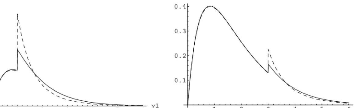
In Figure 1 the density function fi(y1|x)/ψi(x) of the surplus prior to ruin, given it occurs, is plotted for two specific values of initial capital x. Figure 2 depicts both the expected value
E(R−
Tx|Tx <∞, Z0 =i) =
E(R−
Tx1{Tx<∞}|Z0 =i)
ψi(x) and the standard deviation
SDR− Tx = q E((R− Tx) 2|T x <∞, Z0 =i)−E2(R−Tx|Tx <∞, Z0 =i)
as a function of initial capital x. Note that from the analytic expressions above, we see that limx→∞E(R−T
x|Tx < ∞) = 1.86 and limx→∞SDR−Tx = 2.32 (this holds for
bothZ0 = 1,2).
Finally, we briefly illustrate how to use the procedure of Section 5.1 to obtain mo-ments of the time to ruin. From (17), we have for n= 1
A0(s)f~1(s) =c ∂ ~mδ(0) ∂δ δ=0+ ~˜ ψ(s). (45)
1 2 3 4 5 6 y1 0.2 0.4 0.6 0.8 1 1 2 3 4 5 6 y1 0.1 0.2 0.3 0.4
Figure 1: Density function of the surplus prior to ruin, given it occurs, for x = 1 (left) andx= 3 (right) (initial state Z0 = 1 (dashed line) and Z0 = 2 (solid line)).
2 4 6 8 10 12 14 x 0.25 0.5 0.75 1 1.25 1.5 1.75 2 2 4 6 8 10 12 14 x 0.5 1 1.5 2 2.5
Figure 2: Expected value (left) and standard deviation (right) of the surplus prior to ruin, given it occurs (initial stateZ0 = 1 (dashed line) and Z0 = 2 (solid line)).
By analyticity off~1(s) in the right half-plane we thus obtainc∂ ~m∂δδ(0) δ=0=− 7.949 17.841
and thus, after solving (45) and inverting the Laplace transform, we obtain
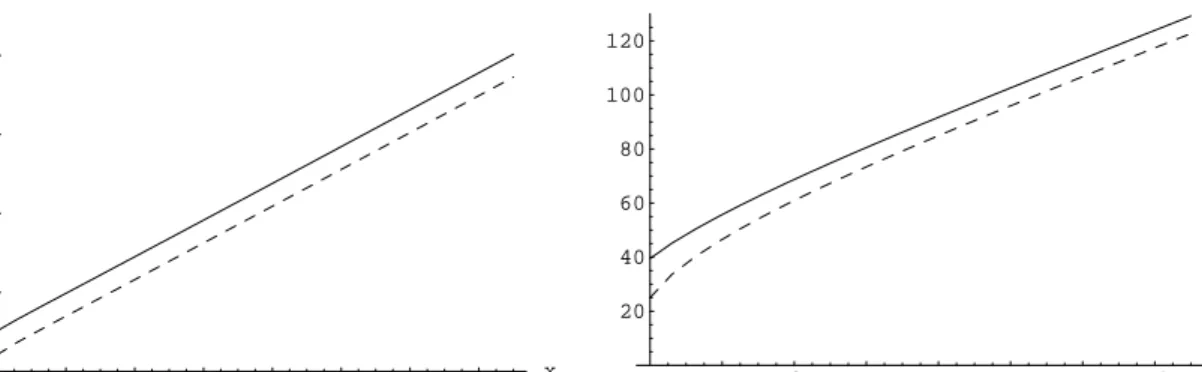
E(Tx1{T x<∞}) = 4.330x+ 4.431 4x+ 9.114 e−0.065x− 0.457 0.193 e−3.161x Analogously, from (17), E(T2 x1{Tx<∞}) = 19.980x2+ 711.096x+ 681.816 18.458x2+ 703.242x+ 1469.25 e−0.065x− 75.458 32.806 e−3.161x. Figure 3 depicts the expected value E(Tx|Tx < ∞, Z0 = i) = E(Tx1{Tx<∞}|Z0=i)
ψi(x) and
the standard deviation of the time to ruin, given it occurs, as a function of initial capitalx. One observes that the standard deviation of the time to ruin exceeds the expected value, so that in this dependency model it is particularly dangerous to just consider the first moment as an indicator for the riskiness of the portfolio strategy. Acknowledgement. The authors would like to thank Clemens Heuberger for help-ful advice on handling determinants.
2 4 6 8 10 12 14 x 20 40 60 80 2 4 6 8 10 12 14 x 20 40 60 80 100 120
Figure 3: Expected value (left) and standard deviation (right) of the time to ruin, given it occurs (initial stateZ0 = 1 (dashed line) and Z0 = 2 (solid line)).
References
[1] I. Adan and V. Kulkarni (2003) Single-server queue with Markov depen-dent interarrival and service times. Queueing Systems 45, 113-134.
[2] H. Albrecher (2005) Discussion on “The time value of ruin in a Sparre Andersen Model” by H. Gerber and E. Shiu. North American Actuarial Journal
9 (2), 71–74.
[3] H. Albrecher and O.Boxma(2004) A ruin model with dependence between claim sizes and claim intervals. Insurance Math. Econom. 35 (2), 245-254. [4] H. Albrecher and J. Teugels(2004) Exponential behavior in the presence
of dependence in risk theory. EURANDOM Research Report 2004-011, TU Eindhoven.
[5] S. Asmussen (2000) Ruin Probabilities, World Scientific, Singapore, 2000. [6] F. Avram and M. Usabel (2004) Ruin probabilities and deficit for the
renewal risk model with phase-type interarrival times. ASTIN Bulletin 34, No.2, 315–332.
[7] A. Badescu, L. Breuer, A. da Silva Soares, G. Latouche, M. Remiche and D. Stanford (2005) Risk processes analyzed as fluid queues.
Scandinavian Actuarial Journal, No.2, 127–141.
[8] Y. Cheng and Q. Tang(2003) Moments of the surplus before ruin and the deficit at ruin in the Erlang(2) risk process. North American Actuarial Journal, 7, 1–12.
[9] J. de Smit(1983) The queueGI/M/swith customers of different types or the queue GI/Hm/s. Adv. in Appl. Probab. 15, 392-419.
[10] D. Dickson(1992) On the distribution of the surplus prior to ruin Insurance Math. Econom.11(3), 191–207.
[11] D. Dickson (1998) Discussion on ”On the time value of ruin” by H. Gerber and E. Shiu. North American Actuarial Journal2(1), 74.
[12] D. Dickson and S. Drekic (2004) The joint distribution of the surplus prior to ruin and the deficit at ruin in some Sparre Andersen models. Insurance Math. Econom.34, 97–107.
[13] D. Dickson and C. Hipp (2001) On the time to ruin for Erlang(2) risk processes. Insurance Math. Econom. 29, 333–344.
[14] G. Doetsch (1937) Theorie und Anwendung der Laplace-Transformation. Springer, Berlin.
[15] F. Dufresne and H. Gerber(1988) The surpluses immediately before and at ruin, and the amount of the claim causing ruin. Insurance Math. Econom.
7(3), 193–199.
[16] H. Gerber and E. Shiu(1998) On the time value of ruin. North American Actuarial Journal, 2(1), 48–78.
[17] H. Gerber and E. Shiu(2005) The time value of ruin in a Sparre Andersen Model. North American Actuarial Journal, 9(2), 49–69.
[18] M. Jacobsen (2003) Martingales and the distribution of the time to ruin.
Stochastic Process. Appl. 107(1), 29–51.
[19] J. Janssen and J. Reinhard (1985) Probabilit´es de ruine pour une classe de mod`eles de risque semi-Markoviens. ASTIN Bulletin 15(2), 123–134.
[20] S. Li and J. Garrido(2004) On ruin for the Erlang(n) risk process.Insurance Math. Econom.34 (3), 391–408.
[21] S. Li and J. Garrido (2005) On a general class of renewal risk process: Analysis of the Gerber-Shiu function. Preprint, Concordia University.
[22] X. Lin and G. Willmot(2000) The moments of the time to ruin, the surplus before ruin and the deficit at ruin. Insurance Math. Econom. 27, 19–44. [23] M. Marcus and H. Minc (1964) A Survey of Matrix Theory and Matrix
Inequalities. Allyn and Bacon, Boston.
[24] L. Sun and H. Yang(2004) On the joint distributions of surplus immediately before ruin and the deficit at ruin for Erlang(2) risk processes. Insurance Math. Econom.34, 121–125.