School of Electrical Engineering, Computing and Mathematical Sciences
Automatically Selecting Parameters for Graph-Based Clustering
Ross Callister
This thesis is presented for the Degree of Doctor of Philosophy
of
Curtin University of Technology
To the best of my knowledge and belief this thesis contains no material previously published by any other person except where due acknowledgement has been made. This thesis contains no material which has been accepted for the award of any other
degree or diploma in any university.
Acknowledgements
Huge thanks to my programme supervisors - Mihai Lazarescu, Duc-Son Pham, and Patrick Peursum, who provided invaluable advice and information, and who amazingly managed to somehow guide me, dazed and confused, to completing this thesis.
I would also like to acknowledge and thank the Australian Federal Government, who generously provided me with the Australian Postgraduate Award (later replaced by the Research Training Program) during my research, which ultimately allowed this work to be produced.
My deepest gratitude goes to my parents, who supported and encouraged me through-out this journey. I love you and appreciate all you’ve done for me. Thank you for being so amazing.
Also to my pets and friends, past and present, thank you for keeping me sane helping me smile at times where smiling was difficult.
Abstract
Clustering data streams is an area of current and active study in the data mining com-munity. Data streams present challenges which are unique and distinct from traditional batch datasets, namely in that each data point may only be read once, there is a poten-tially unlimited number of data points to cluster, and that the distribution of the data points may vary over time. This final challenge requires that the algorithm be able to adjust itself to match the changing distributions as they arise.
Because clustering is an unsupervised process, setting the input parameters cor-rectly is of vital importance, and can greatly affect the quality of clusters produced by a clustering algorithm. However, in a data stream the distribution of the data can change over time. This means that not only is it a challenge to set initial input param-eters appropriately, but the paramparam-eters used for clustering may not be appropriate at different times during the stream. In this thesis we address this issue for the state-of-the-art clustering algorithm - RepStream by removing the need to set and update the critical K parameter. This leads us to introduce the RobustRepStream algorithm, an extension to its predecessor which is designed to adapt to some of the most difficult challenges facing stream clustering algorithms.
Our first major contribution is a demonstration that features computed from the structure of the K-nearest neighbour sparse graph used by RepStream can be used to detect change in the distribution of the dataset. We do this by computing several fea-tures based on the internal K-nearest neighbour graph structure and using a change detection algorithm on these features to show that they vary over time as the stream distribution changes. This in turn provides evidence that changes in the data
distribu-tions are measurable and can be used to help algorithms adapt to the changes.
Secondly, we introduce the anomalous edge score, which is a feature computed from theK-nearest neighbour structure of RepStream. The anomalous edge score rep-resents the number and relative length of edges which are significantly longer than average for any given vertex. We study the average anomalous edge score for a range ofK values on various dataset and suggest that changes in the value of the score corre-spond to changes in the value of the optimumK value. By introducing a threshold to the anomalous edge score we can continuously selectK values in RepStream over the length of the stream which perform comparably well compared to the optimalKvalue at each time step.
Next, we modify and extend RepStream to automatically vary theK parameter for newly added data points in response to the changing anomalous edge score. We adjust the K parameter based on a threshold in a single live instance of RepStream. Setting theK parameter in RepStream was difficult as different datasets had different optimal values, and in data streams the optimalKvalue could vary over time as the distribution changed. We demonstrate that by adjusting theK value for new incoming data points we can continuously select and update its internalKvalue which produces high quality clustering results over time in data streams.
Finally, we propose RobustRepStream, an extension of the RepStream algorithm, to automatically select the number of outgoing edges for newly added data points in response to the changing skewness excess score. RobustRepStream causes the number of outgoing edges for each vertex to be no longer dependent on a staticK value. We demonstrate that this method constructs nearest neighbour graphs without the need for specifying a specific number of outgoing edges, which removes the need to set the most critical and sensitive parameter of RepStream.
Published Work
This thesis includes material from the following works that have been published over the course of the Ph.D research. They are listed along with the corresponding chapters within this thesis.
• Article 1 (Chapter 2,3) -Callister, R., Lazarescu, M., & Pham, D. S. (2015). Detection of Structural Changes in Data Streams. In Proceedings of the Thir-teenth Australasian Data Mining Conference (AusDM 2015), Sydney, Australia,
August 2015(pp. 79-88).
• Article 2 (Chapter 4) - Callister, R., Lazarescu, M., & Pham, D. S. (2017, April). Graph-based clustering with DRepStream. InProceedings of the
Sympo-sium on Applied Computing(pp. 850-857).
• Article 3 (Chapter 2,4) -Callister, R., Pham, D. S., & Lazarescu, M. (2019). Using distribution analysis for parameter selection in RepStream.Mathematical
Foundations of Computing, 2(3), 215-250.
• Article 4 (Chapter 2,5) -Callister, R., Pham, D. S., & Lazarescu, M. (2020). RobustRepStream: Robust Stream Clustering Using Self-Controlled Connectiv-ity Graph.Intelligent Data Analysis, 24(4).
Statement of Contribution by Others
Articles in the following attribution tables are numbered according to the list of published works on the previous page. This represents contributions to the following papers by the listed co-authors.Attribution of Dr. Duc-Son Pham Article Literature Review Concept Design Software Modelling Experimental Results Data Analysis Discussion Paper Writing 1 X 2 X 3 X X 4 X X
Attribution of Dr. Mihai Lazarescu Article Literature Review Concept Design Software Modelling Experimental Results Data Analysis Discussion Paper Writing 1 X 2 X 3 X 4 X Ross Callister. ... Dr. Duc-Son Pham... Dr. Mihai Lazarescu...
Contents
Acknowledgements v
Abstract vii
1 Introduction and Motivation 1
1.1 Data Stream Clustering . . . 2
1.2 Problems With Stream Clustering . . . 6
1.3 Problem Statement . . . 9
1.4 Contributions . . . 11
1.5 Thesis Structure . . . 12
2 Background and Literature Review 15 2.1 Change Detection Background . . . 15
2.1.1 Approaches Including Change Detection . . . 16
2.1.2 Anomaly detection . . . 16
2.1.3 Stream Change Detection Methods . . . 17
2.2 Stream Clustering Algorithms . . . 18
2.2.1 Micro-Cluster/Density-Based Clustering . . . 18
2.2.2 Grid-Based Clustering . . . 21
2.2.4 Other Novel Clustering Methods . . . 27
2.2.5 Parameters In Clustering . . . 29
2.3 The RepStream Algorithm . . . 32
2.3.1 Point Level Sparse Graph . . . 33
2.3.2 Representative Level Sparse Graph . . . 34
2.3.3 Clustering With RepStream . . . 36
2.3.4 Algorithm . . . 37
2.3.5 Parameters In RepStream . . . 41
3 Change Detection 43 3.1 Overview of Stream Change Detection . . . 43
3.1.1 Contributions . . . 46
3.2 Definitions . . . 46
3.2.1 Basic Definitions . . . 46
3.2.2 Feature Definitions . . . 48
Cluster Count . . . 48
Edge Change Count . . . 49
Cluster Merges and Splits . . . 51
Edge-Length Variation . . . 52
History Count . . . 52
3.3 Methodology . . . 54
3.3.1 Feature Extraction . . . 54
3.3.2 Detection Scheme . . . 54
3.3.3 Defining Ground Truth Changes . . . 56
3.4 Experiments . . . 59
3.4.2 Dataset . . . 60
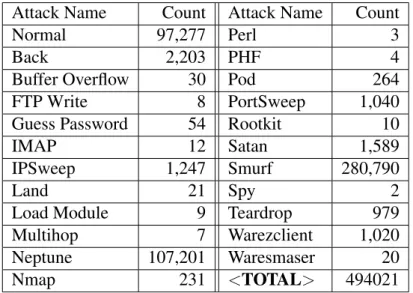
KDD Cup 99’ . . . 60
KDD Dataset Composition . . . 61
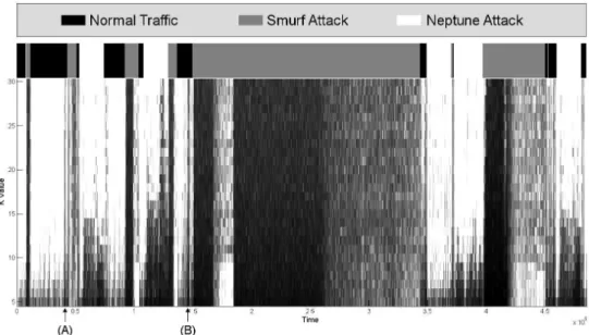
Smurf Attack . . . 62
Nepune Attack . . . 63
Normal Traffic and Other Attacks . . . 63
3.4.3 Feature Evaluation . . . 65
3.4.4 Setup and Parameter Selection . . . 71
3.4.5 Results . . . 73
3.5 Discussion . . . 75
3.5.1 Qualitative Analysis . . . 76
3.5.2 Comparison Method Analysis . . . 78
3.5.3 Parameters . . . 79
3.5.4 Summary . . . 79
3.6 Conclusion . . . 81
4 SelectingK in RepStream 83 4.1 DynamicK Selection Overview . . . 83
4.2 Proposed Method . . . 86
4.2.1 Inter versus Intra Class Edges . . . 86
4.2.2 Edge Distribution Score . . . 88
4.2.3 Selection of theKParameter . . . 92
4.3 Evaluation . . . 94
4.3.1 Synthetic Datasets . . . 94
DS1 and DS2 . . . 94
Closer . . . 97
4.3.2 Benchmark Datasets . . . 98
The KDD Cup 1999 dataset . . . 98
The Tree Cover Type dataset . . . 99
4.3.3 Experimental Set-Up . . . 99
4.3.4 Results vs Other Algorithms . . . 100
4.3.5 Results vs RepStream . . . 110 4.4 Discussion . . . 115 4.5 Conclusion . . . 116 5 RobustRepStream 117 5.1 Overview of RobustRepStream . . . 117 5.2 Proposed Method . . . 120 5.2.1 Skewness Excess . . . 121 5.2.2 RobustRepStream . . . 125 5.3 Experiments . . . 131
5.3.1 Real World Data Sets: KDD and Tree Cover . . . 131
The KDD Cup 1999 data set . . . 131
The Tree Cover Type Data Set . . . 132
5.3.2 Synthetic Data Sets . . . 132
Closer Data Set . . . 132
SynTest Data Set . . . 133
Shapes Data Set . . . 134
DS1 and DS2 . . . 134
5.3.3 Evaluation Metrics . . . 136
5.3.5 Baseline for Comparison . . . 141 5.3.6 Evaluation of RobustRepStream . . . 146 5.3.7 Sensitivity . . . 148 5.4 Results Discussion . . . 150 5.5 Conclusion . . . 151 6 Conclusions 153 6.1 Change Detection . . . 154
6.2 Dynamic K Parameter Selection . . . 154
6.3 RobustRepStream . . . 155
6.4 Future Work . . . 156
List of Figures
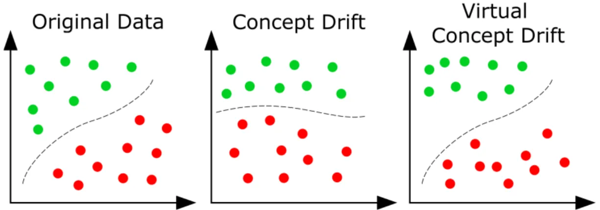
1.1 Real and virtual concept drift. Colours represent members of different classes. . . 6
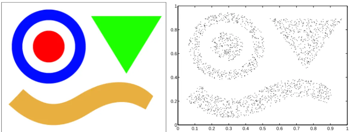
1.2 The underlying classes in a stream versus data points sampled from the same set of classes. . . 8
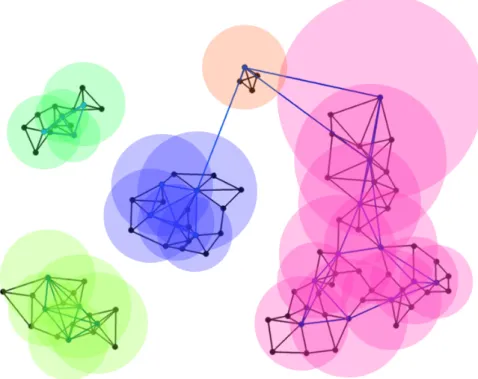
2.1 An illustration of the representative and point-level sparse graphs in the RepStream algorithm. . . 34
2.2 Representative compared to point-level sparse graphs. . . 35
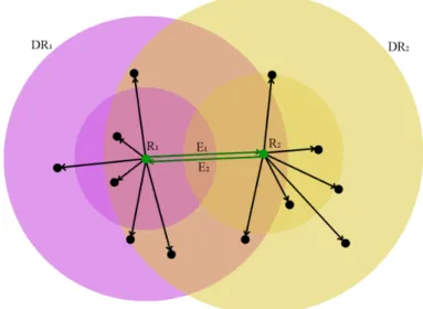
2.3 The density relation radius of a representative point is equal to α×
AvgDist whereAvgDist is the average distance to itsK-nearest
neigh-bours. . . 38
2.4 An example of two representative points which are both reciprocally connected, and density related. . . 38
2.5 An example of two representative points which are reciprocally con-nected, but not density related. . . 38
2.6 Density relation radii for the representative points in the hypothetical example in RepStream. The distance to the neighbours at the point level determines the density relation radius for the representative level clustering. . . 39
3.1 Example of distribution change in a stream. Distribution A shows two classes of the same density at different spacial locations. At a later time in the data stream, distribution B, the red cluster has shifted its position, whilst the blue cluster has increased its size, and decreased
its density. . . 47
3.2 Cluster Count. In this example at T =1 there are 3 clusters. The addition of an extra point at T =2 results in two clusters merging, reducing the cluster count to 2. . . 49
3.3 history count. PointP1begins in clusterC1initially, then at timeT =2 the addition of a new data point causes a change in the membership to clusterC2. Later atT =3 it returns to the cluster it was previously in. 53 3.4 Flowchart showing feature extraction, detection on each feature, then majority voting to reach the final change detection decision. . . 56
3.5 Illustrative example of the F-Measure heatmap. . . 57
3.6 The heatmap of the KDD 99’ Dataset, with change points marked. . . 61
3.7 Locations of the three most common classes in the KDD Dataset, with heatmap. . . 64
3.8 Raw feature data taken from the KDD dataset with the heatmap for comparison. . . 66
3.9 Raw feature data taken from the KDD dataset with the heatmap for comparison. . . 67
3.10 Detected change points using individual features. . . 71
3.11 Our moving average detection algorithm on the KDD dataset. . . 73
3.12 PCA Change Detection algorithm run on the KDD dataset. . . 73
3.13 ROC Curve of the two methods, using curve-fitting. AUC is 0.9888 for the proposed method and 0.7298 for the PCA based method. . . . 74
4.1 Intra and Inter-class edges. The Edge E1 is considered an inter-class edge as it connects two vertices R1 and R2 that belong to different ground-truth classes. EdgeE2 connects two vertices belonging to the
same class and thus is considered an intra-class edge. . . 88
4.2 An illustration of relative edge lengths of nearest neighbours in the middle of a cluster versus near the edge of a cluster. . . 89
4.3 Different cases for the distribution of edge lengths. . . 91
4.4 Visualisation of the DS1 dataset. . . 95
4.5 Visualisation of the DS2 dataset. . . 95
4.6 Two dimensional representations of the 5 classes in the SynTest dataset. The main class is always present and steadily changes shape, the smaller classes appear at various points through the dataset, as shown in Figure4.7. . . 96
4.7 The class presence of the classes in the SynTest dataset. A marker indicates that the class is present in the dataset during the given time window. . . 96
4.8 The evolution of the Closer dataset, showing slices of its 3 sections.. . . 97
4.9 Comparative purity for Tree Cover dataset . . . 101
4.10 Comparative purity for Tree Cover dataset . . . 101
4.11 Comparative purity for KDD 99’ Cup dataset . . . 102
4.12 Comparative purity for KDD 99’ Cup dataset . . . 103
4.13 Comparative purity for DS1 dataset . . . 104
4.14 TheKvalue selected by our dynamicK method on the DS1 dataset . . 104
4.15 Comparative purity for DS2 dataset . . . 105
4.16 Comparative purity for SynTest dataset . . . 106
4.17 Comparative purity for Closer dataset . . . 107
4.18 Comparative purity for Tree Cover dataset . . . 107
4.19 Comparative purity for KDD 99’ Cup dataset . . . 108
4.21 F-Measure comparison vs RepStream using optimal parameters on DS1 dataset . . . 111
4.22 F-Measure comparison vs RepStream using optimal parameters on DS2 dataset . . . 111
4.23 F-Measure comparison vs RepStream using optimal parameters on Syn-Test dataset . . . 112
4.24 F-Measure comparison vs RepStream using optimal parameters on Closer dataset . . . 113
4.25 F-Measure comparison vs RepStream using optimal parameters on Tree Cover dataset . . . 113
4.26 F-Measure comparison vs RepStream using optimal parameters on KDD 99’ Cup dataset . . . 114
5.1 Intra and Inter-class edges. The Edge E1 is considered an inter-class
edge as it connects two vertices R1 and R2 that belong to different
ground-truth classes. Edge E2connects two vertices belonging to the
same class and thus is considered an intra-class edge. . . 122
5.2 An illustration of relative edge lengths of nearest neighbours in the middle of a cluster versus near the edge of a cluster. . . 122
5.3 Histograms of normalised edge lengths for variousKvalues . . . 125
5.4 Average SE vsK, normalised with respect to MAD . . . 126
5.5 Histogram showing the distance to the nearest 200 vertices in a 400 point 2 dimensional normal distribution, with the origin at the centre of the distribution. Standard deviation is 100 in both the x and y direction.126
5.6 Nearest neighbour plot of a 400 point 2 dimensional normal distri-bution with a standard deviation of 100. Plot shows the 200 nearest neighbours from the centre of the distribution. . . 127
5.8 Two dimensional representations of the 5 different classes. The main class is always present and steadily changes shape, the smaller classes appear at
various points through the data set, as shown in Figure5.9. . . 134
5.9 The class presence of the classes in the SynTest data set. A marker indicates the class is present in the data set during the given time window.135 5.10 The first and second stage of the Shapes data set. . . 135
5.11 DS1 and DS2 datasets. . . 136
5.12 Comparative purity for TreeCov dataset. . . 138
5.13 Comparative purity for KDD dataset. . . 139
5.14 Comparative purity for our Synthetic datasets against D-Stream and DBStream. . . 142
5.15 Comparative purity for KDD Cup 99’ data set . . . 143
5.16 Comparative purity for Tree Cover data set . . . 143
5.17 F-Measure scores for RobustRepStream versus optimally-parametrised RepStream . . . 145
5.18 Results for the KDD data set. . . 146
5.19 Results for the Tree Cover data set. . . 147
Chapter 1
Introduction and Motivation
It has been predicted that in the current age of information, the total amount of data generated and stored in all human history will double approximately every two years for the foreseeable future (Zwolenski et al., 2014). This massive explosion in data is thanks to the rising popularity and use of things such as:
• Sensor networks(Kumar et al., 2017) used for monitoring the state of equipment
or the environment.
• Location data(Zhao et al., 2016) from GPS systems built into cars, smartphones,
animals for behavioural research, and other devices.
• Social networking data(Imran et al., 2018) from online networks such as Twitter
and Facebook, in which huge amounts of interactions occur every second.
• Web metadata, such as clickstream analysis (Wang et al., 2017) which provides
analytics services for website administrators.
• Cloud computing(Botta et al., 2016) with the need for analysis and optimisation
of usage being an ever more important thing.
• Smart-connected devicessuch as the Amazon Alexa or Google Nest which
With the huge rise in captured data comes a proportional increase in demand for data-mining techniques, and in order to make use of this torrent of new data the field of data stream mining has arisen. Such streams present a number of constraints (Ag-garwal, 2015), specifically their unbounded length, the infeasibility of storage, the one-pass constraint, concept drift, the rate of data generation, and the vast amounts of metadata which must be handled.
Data mining techniques used on data streams can include supervised classification, outlier detection, and pattern mining, however stream cluster analysis is the topic on which we focus in this work.
Cluster analysis is regarded as the primary objective of unsupervised data mining (Gorunescu, 2011), and is a vital tool in exploratory data mining. While on the surface it may seem like a trivial and intuitive task to determine which members of a group are similar and which are dissimilar, this task is actually incredibly complex in an unsupervised context, and is abound in edge cases and subjective judgements. This has led to a wide and varied field of research into determining better ways of clustering data, particularly, in recent times, on data streams.
1.1
Data Stream Clustering
Data streams continue to become a more common feature of study thanks to their prevalence in the computing sphere. Streams generated by sensor networks, online interaction, business or market data, and video streams contain huge amounts of data which can be mined to gain useful, practical insights (Barddal, 2019). Particularly, stream clustering is an informative process, which involves the unsupervised separation of data points into groups, called clusters.
Data streams are typified by a series of data arriving sequentially over time. This data may be numerical, categorical, binary, images, video, audio, or any one of a multitude of different types. This thesis concentrates on multi-dimensional numerical data, which can be expressed as vectors in hyperspace.
Definition 1.1.1 A data streamS is a set of vectors X1,X2, . . . which is unbounded in length and ordered by time:
S ={X1,X2, . . . ,Xm. . .} (1.1)
with each vectorXiin the stream being composed of a number of attributes -Xi=
{xi,1. . .xi,d} - where d is the dimensionality of the stream, the number of attributes
associated with each data point. Each attribute of a data point has a real value, such that the data point can be represented as a point ind-dimensional space.
The values of these attributes define the location of the vector in the hyperspace. The attributes making up each data point are also alternatively referred to as data di-mensions, observations, features, or components.
Using clustering algorithms we seek to group the vectors from the data set into groups of similar data points, as distinct from data points which are dissimilar (Berkhin, 2006; Charu & Chandan, 2013). The fundamental steps of clustering (Gorunescu, 2011) are:
• Defining a similarity measure between data points.
• Defining a method to construct clusters based on the similarity measure.
• An algorithm which incrementally changes clusters as new data points arrive from the stream.
Similarity between data points is defined according to a given distance metric. Most commonly, the Euclidean distance, Manhattan distance, or Manhattan Squared distance measures are used due to their simplicity and intuitiveness (Jain et al., 1999). However, other more sophisticated distance measures are occasionally used including the Mahalanobis distance measure (Mao & Jain, 1996). While alternative distance metrics can address problems related to Euclidean and Manhattan distances, namely
that attributes with greater scales tend to dominate over the smaller scaled ones, an-other common solution is to normalise each dimension of the incoming data points, such that the scales of each is equal.
In both stream and batch clustering methods, data points are grouped based on their distance from each other using a chosen distance metric. Thus, the process is to separate the data points{X1,X2...Xk...}into subsets known asclusters, by mapping each point to one of a series of clustersC1,C2, . . .Cj. . .. These clusters are meant to approximate distinct concepts within the dataset, and describe different regions of the data. As such, clusters represent a model of the hidden underlying concepts of the stream, and this is what makes clustering an unsupervised process - that training data and validation data is unavailable to the algorithm. Clusters typically do not intersect within the data space, although exceptions exist.
Stream clustering is typically a process used on batches too large to fit entirely into memory, or unbounded streams of data, in which clusters must be produced ei-ther incrementally over time, or at user-specified times. Clusters can be used to locate sub-groups within a complex dataset, and to identify relationships between members of the stream. Cluster analysis has been used in a rage of applications such as mar-ket research, image analysis (Li et al., 2018), medical analysis (Camara et al., 2019), genome clustering (Wang et al., 2019), recommender systems (Logesh et al., 2019), and anomaly detection (Aytekin et al., 2018), and so reliable performance when deal-ing with datasets where little is known is important.
Due to the streaming nature of the data the membership of the clusters can change over time, with data points swapping from cluster to cluster, or being added to new clusters as the clustering algorithm dictates. Data streams have a series of requirements (Cao et al., 2006), specifically:
• The number of clusters can’t be assumed. • Clusters may be of arbitrary shape and size.
As such, clusters are typically thought of as contiguous regions of the data space which contain data points at a relatively high level of density, separated by regions of space with a significantly lower density or containing no points at all.
There are various approaches that are used to perform clustering, with one of the earliest being the well-knownK-means algorithm (MacQueen et al., 1967), which is a partition-based approach. While the K-means algorithm was designed for batch datasets rather than streams, later approaches have applied the K-means algorithm to the streaming context (Ackermann et al., 2012). The limitation of theK-means algo-rithm is that the number of desired clusters must be specified, and the algoalgo-rithm is only capable of finding convex clusters. To address these limitations, there are a wealth of other more sophisticated approaches (Aggarwal, 2015, 2007; Charu & Chandan, 2013) including micro-cluster and density based methods, graph-based methods, grid-based methods, agglomerative and divisive hierarchical approaches, and even unique evo-lutionary or biologically-based clustering approaches. These other approaches have their own limitations and requirements. Micro-cluster and density based approaches, for example DenStream (Cao et al., 2006), typically do not require a number of clusters to be specified, however density threshold and micro-cluster size parameters typically need to be given by the user. Graph-based approaches, such as ExCC (Bhatnagar et al., 2014) and PatchWork (Gouineau et al., 2016), similarly typically require den-sity thresholds and grid size parameters to be set by the user. Graph-based approaches often use nearest-neighbour graphs like SNCStream (Barddal et al., 2015), or mini-mal spanning trees like HASTREAM (Hassani et al., 2014), which require parameters to determine connectivity, or thresholds for cluster construction after hierarchical tree splitting has occurred. As we see, whilst more sophisticated approaches can operate without specifying the number of clusters, they each have their own requirements for parametrisation.
Despite the large variety in algorithms designed to perform clustering on data streams, it is far from being a solved field. Cluster analysis remains a foundational part of gaining useful knowledge from data, and so achieving high quality clustering
Figure 1.1: Real and virtual concept drift. Colours represent members of different classes.
is an important goal.
1.2
Problems With Stream Clustering
Originally, cluster analysis was a task to be performed on batches of data - algorithms mapping each data point in a static data set to a cluster, with the data being accessible multiple times and at will, and having a finite number of data points to process. As technology advanced and requirements changed the need arose for clustering to be performed on data streams.
Streams introduce multiple significant challenges compared to batch data, specifi-cally:
• The data stream is potentially endless, so storing every data point is infeasible. • Data points may be read from the stream only once, in the order that they arrive. • The distribution of data points from the stream can change over time, requiring
entirely different cluster mapping at different periods in the stream.
According to Schlimmer & Granger (1986), concept attainment is a field of ma-chine learning in which one seeks to create a model learning to separate data points into specific concepts. These concepts represent a priori divisions of the data space
into distinct categories. The idea behind learning these concepts and building a model to represent them is to successfully predict the concept to which a new unseen instance of data belongs to. Concept attainment includes supervised tasks like classification us-ing trainus-ing data, as well as unsupervised learnus-ing like clusterus-ing, in which no trainus-ing data is used.
According to Gama et al. (2014), in machine learning, concept drift occurs when the underlying concepts change over time.
Definition 1.2.1 Concept drift occurs when the probability of a set of input variables X being mapped to a target variable y changes over time. In the context of data clus-tering, it is the probability that the observed data points, X will be correctly mapped to the ideal ground-truth classes y over time, which can be defined as:
∃X:pt
0(X,y)6=pt1(X,y), (1.2)
where pt0(X,y) represents the joint probability distribution of the data at time t0
between the set of input data points X and the distribution classes y, and likewise
pt1(X,y)represents the joint probability of pointsX and classesyat the later timet1. In reality we can only observe the unlabelled data points as they arrive from the stream - i.e. we only observe p(X)over time (Gao et al., 2007). This makes it hard to determine whether the change is merely a change in sample population or real concept drift.
Real concept drift occurs when the probability of a given observation belonging to a given class changes over time - whenp(y|X)changes. Virtual concept drift, however, occurs when the population shifts, but the probability of an observation belonging to a given class doesn’t change - when p(X)changes, but p(y|X)remains the same (Gama et al., 2014).
In the context of clustering, and this thesis, we are interested in real concept drift that affects the predictive power of clustering algorithms - changes in the underlying concepts in the stream over time. Since clustering is an unsupervised process we have
0 0.1 0.2 0.3 0.4 0.5 0.6 0.7 0.8 0.9 1 0 0.2 0.4 0.6 0.8 1
Figure 1.2: The underlying classes in a stream versus data points sampled from the same set of classes.
only the data points sampled from these underlying concepts available for observation. Adjusting to handle such changes in concept involve predicting changes in concept by examining the changes in population distribution of time.
Changes in data distribution, known asstream evolutionorconcept drift, is a partic-ularly challenging property of data streams (Hulten et al., 2001). The data points from the data stream are sampled from an underlying set of classes, which ideally would map to clusters in the stream clustering context, as illustrated in Figure1.2. The goal of cluster analysis is to discover and approximate these classes, and to map the given data points to clusters representative of them. Over time, these classes can change in density, move within the data space, merge, split, disappear, emerge, change size, ro-tate, or change shape. This would result in changes to the distributions of sampled data points. Such changes in underlying distribution can happen abruptly, or gradually over time, and both kinds of evolution can impact the integrity of clustering results if the algorithm is not designed to deal with it. In addition, noise in the stream can impact clustering in the same way that evolution does.
Stream evolution poses several challenges which have significant implications for stream clustering algorithms. Firstly, stream evolution means that older data may be less and less representative of the current data distribution as time goes on (Aggarwal, 2018). This can lead to algorithms defining clusters based on older data which is no longer relevant for the current state of the stream. This problem is often addressed
using fading functions and decay of older data, in which newer data is prioritised in clustering and older data is weighted less, or gradually removed over time (Khalilian & Mustapha, 2010). A trade-off is inevitable between the consideration of historical data points in clustering decisions, and focusing on newer data points to reduce the possibility of basing clustering decisions off of data which is no longer relevant. This trade-off is often left to the user in the form of a parameter which affects the rate at which older data is made redundant.
Secondly, as the stream evolves over time the distribution of data can change in un-predictable ways such that the underlying classes are completely different at different times in the stream. Clustering algorithms typically rely on user-specific parameters which represent thresholds, or similar values, which affect how the algorithm groups data points into clusters. Setting these parameter values inappropriately can lead to clustering output which is meaningless, yielding little or no useful knowledge about the data. It is imperative that the parameters are set well in order to achieve useful clustering results. However, a major issue with stream clustering is that even if the ini-tial parametrisation of the stream clustering algorithm results in high-quality clustering output at one point in the stream, concept drift may mean that those same parameters are no longer appropriate later in the stream.
1.3
Problem Statement
In light of the above issues, our purpose in this thesis is to achieve higher and more consistent quality clustering output in a streaming context. Particularly we wish to develop methods which respond to changes in the underlying data stream, and which are more robust to concept drift, requiring as little parametrisation by users as possi-ble. Clustering is an unsupervised process, where often little, if anything, is known about the dataset prior to analysis. As such, algorithms which require users to specify parameters which are very sensitive to the data distribution are not robust with respect to unpredictable stream evolution. One of the greatest challenges in stream
cluster-ing is buildcluster-ing algorithms without requircluster-ing ad-hoc critical parameters such as cluster number, density, grid granularity, graph connectivity, or window length (Silva et al., 2013). We propose, therefore, that it is vital for algorithms to consider concept drift with respect to algorithm parametrisation. It is vital to make these input parameters less sensitive, or, preferably, to reduce the number of input parameters a user must set, so as to achieve more robust and reliable clustering.
Because of the issues with stream clustering our motivation is to adapt to concept drift within the data streams in a stream clustering context. The first method for adap-tation is by identifying when these changes occur. Such a process is known aschange
point detection. Firstly we wish to demonstrate that concept drift is detectable
algorith-mically by analysis of geometric and distributional properties of the stream clustering model. By employing change point detection methods we wish to identify when stream evolution occurs. Change point detection is itself an area of study in statistical anal-ysis (Truong et al., 2018), and we wish to use it to identify when changes occur in arbitrarily dimensional data streams, as defined earlier. By analysing the geometric and structural properties of the multi-dimensional stream data we propose that these change points can be identified. Our goal is to create a method for reporting when change points happen in the underlying data as the stream progresses.
Secondly, we wish to improve the robustness of clustering algorithms. Specifically in this thesis we concentrate on the nearest-neighbour graph-based clustering approach. Typically this kind of clustering involves setting aK connectivity parameter, which is sensitive and must be set correctly for useful clustering to occur. K-nearest neighbour (KNN) graph-based stream clustering algorithms are able to detect arbitrarily shaped clusters with arbitrary levels of density, this results in high quality clustering output at the expense of a higher level of computational complexity provided that theK param-eter is set appropriately. Our goal is to reduce the sensitivity of the critical clustering parameters used in this method of clustering, making it less sensitive to stream evo-lution. We do this by computing features based on the relative distances of edges connecting to nearby neighbours in theKNN graph structure, and using these features
to inform clustering.
1.4
Contributions
The contributions of this thesis are:
• A thorough review of related background literature in Chapter2, particularly in regards to current stream clustering approaches. We show their methods, cat-egorise them by their approaches, and describe their various input parameters. We show that clustering relies on sensitive input parameters which must be set by users.
• A change point analysis algorithm for use in a multi-dimensional data stream in Chapter3, which uses features computed from the nearest-neighbour structure of RepStream.
• A method for the analysis of the geometrical and statistical features in Rep-Stream’s graph structure to evaluate the effectiveness of the currentK connectiv-ity parameter, and to indicate when and in which direction it should be changed over time in Chapter4. This is achieved through the use of theedge distribution
score, which is a statistical measure computed from the edges in the K-nearest
neighbour structure in RepStream. The edge distribution score approximates how much the edge length distributions differ from the expected distribution, and allows us to infer properties of the local neighbourhood.
• An extension of RepStream in Chapter4which automatically varies its K con-nectivity parameter in response to changes in the edge distribution score. We show how the thresholding parameter is relatively insensitive and robust com-pared to the sensitiveK parameter which must be set and remains static during the whole stream in the original RepStream version.
• A method for controlling the local connectivity of vertices in a nearest-neighbour sparse graph, in Chapter 5, through the analysis of the skewness excess score,
which quantitatively measures the relative skewness excess of the local neigh-bourhood in a nearest neighbour graph. We show how this measure can be used to approximate an appropriate level of connectivity of a vertex in its local neigh-bourhood.
• The RobustRepStream algorithm in Chapter 5, an extension of the RepStream algorithm which removes the need for the user to set theKparameter entirely by using the skewness excess score. We show that this algorithm is robust across varied types of datasets, both on real-world and synthetic datasets.
1.5
Thesis Structure
Our thesis structure is as follows:
Firstly in Chapter 2 we present a thorough background and review of literature regarding stream clustering methods with respect to evolution of data streams. Specif-ically, we show the prevalence and importance of initial input parameters to the al-gorithms. Whilst the algorithms are often very different in which parameters must be specified by users, all the algorithms require some level of parametrisation and as-sumptions that must be made about the data. The papers reviewed in this chapter cover algorithms which deal with stream evolution via various techniques, and also covers a variety of different classes of clustering algorithms.
Having showed the wide variety of clustering approaches and their reliance on input parameters, in Chapter3we propose a method for detecting concept drift within data streams that evolve over time. Given that the evolution of concepts in the stream directly relates to the effectiveness of the input parameters, being able to measure and detect when this change occurs is paramount. We show that high-level computed features can be effectively used to identify when stream evolution takes place, and we experimentally show that our method performs better than other related stream change detection methods.
features to produce more robust clustering. Given that stream evolution can be detected using these features, we hypothesise that they could also allow critical input parameters to be adjusted over time to produce better clustering. Thus, we present our extended version of RepStream, which uses a novel concept called theedge distribution scoreto determine an appropriate level ofK connectivity in RepStream’sK-nearest neighbour sparse graph structure. Using the edge distribution score to automatically control theK
connectivity over time, we show that we can achieve clustering performance which is comparable to that of RepStream when the theoretical bestKparameter is set. We also show that our method achieves performance which is superior to other contemporary, sophisticated stream clustering approaches.
While allowing parameters to be automatically adjusted to more appropriate val-ues over time in response to stream evolution is a good step, perhaps a better solution is reducing the number and sensitivity of parameters that clustering algorithms rely on. In Chapter5we introduce the RobustRepStream algorithm which performs stream clustering without the need for the user to set the sensitiveK parameter, which is the primary parameter of the RepStream algorithm. We introduce the concept of skewness excess, which is used by the proposed RobustRepStream algorithm to automatically determine appropriate levels of connectivity in its sparse graph structure without the need for aK parameter. With the user no longer responsible for determining the crit-icalK parameter, we show that RobustRepStream produces consistently high quality clustering across all of the datasets we evaluate on, with no changes in input parameter values.
Chapter 6 concludes this thesis. We discuss the proposed methods in regards to handling data stream evolution and parameter sensitivity in clustering algorithms, as well as possible directions for future work.
Chapter 2
Background and Literature Review
Our research focuses on the adaptation of clustering algorithms to changes in a data stream over time, otherwise known as concept drift, or stream evolution. This chter reviews the lichterature related to change detection in data streams, as well as ap-proaches that have been used to adapt to concept drift in order to mitigate the problems it presents.
The literature reviewed in Section2.1examines clustering methods which analyse incoming data for distributional changes, as well as stream change detection meth-ods. In Section 2.2 we examine various stream clustering algorithms, particularly in analysing the hyper-parameters used by each approach. This covers the different stream clustering approaches, including micro-cluster based, grid-based, and graph-based methods, as well as other approaches.
2.1
Change Detection Background
Data streams, as we discussed in the previous chapter, are characterised by evolving data. Data evolution poses major challenges to data mining algorithms, and so re-searchers have applied many techniques to address it (Khamassi et al., 2018). Concept drift is closely related to the idea of change detection in statistics, and so many tech-niques have been proposed which are inspired by change detection methods. Here we present an overview of such techniques, which seek to identify when change occurs, so that the knowledge can be used to better understand emerging concepts in the stream.
2.1.1
Approaches Including Change Detection
There are some clustering approaches which do use change detection mechanisms in their operation, either for the purposes of remaining consistent with newer data, or for discovering new concepts as they emerge. The grid-based algorithm clustering algorithm ExCC (Bhatnagar et al., 2014) uses a novel approach to handling drift in stream distribution. When new points are outside expected boundaries in ExCC they are added to a ‘hold queue’, which is periodically examined to determine whether change has occurred. If a sufficient number of new points are outside expected ranges then a ‘change’ is reported, otherwise it is counted as an outlier or short-term temporary drift. This method can be thought of as a form of detecting stream change, in the case of ExCC it is change within the position of new points on a grid. This is an example which does not use standard statistical methods of change detection. ExCC is described in more detail in Section2.2.
An approach by (Masud et al., 2011) proposes a method for detecting the appear-ance of new classes in a data stream clustering context by deferring classification of outliers and placing them in a buffer, then analysing the points in the buffer for cohe-sion representing a novel class. This method detects the appearance of new classes in a stream, which is relevant to the field of cluster analysis and especially given that one of our primary goals is to adapt to emerging classes. Other topics related to change detection in data streams include recording and tracking change over time for the iden-tification of temporal change (Dunham & Hahsler, 2011), or tracking change in a noisy stream through cluster density analysis (Nasraoui & Rojas, 2006).
2.1.2
Anomaly detection
Anomaly detection is a related field which seeks unexpected or anomalous inputs which may be used for data streams. (Chandola et al., 2009) categorise anomaly detection approaches into the following categories. Classification-based approaches construct a classifier using training data, then classifies new data points into one of the learned classes, examples of which are provided by (Janssens et al., 2009). Nearest-neighbour based approaches use a distance measure between data points and either take the distance to its kth nearest neighbour, or which calculate a density based on distance to neighbouring points.
An example is iNNE (Bandaragoda et al., 2014) which attempts to isolate new points from its nearest neighbours to calculate an anomaly score. Clustering-based
approaches use clustering algorithms to group normal data into a series of clusters, and new data points are considered to be anomalous or not depending on whether they match an existing cluster for instance (Rajasegarar et al., 2014) uses clustering algorithms on distributed sensor networks and examines the inter-cluster distance for anomalous data.
Statistical anomaly-based techniques compare new points to a model and gener-ate either an anomaly score or perform a hypothesis test to probabilistically determine when change occurs (Soule et al., 2005). Some more novel techniques use other con-cepts such as spectral methods, for example a paper by Pham et al. (2014) which uses residual subspace analysis to detect anomalies in a compressed form of the data stream. These algorithms are somewhat similar in concept to change detection, concentrating on unexpected transient changes which differ from what is considered to be ‘normal’ behaviour. Anomaly detection can, in a sense, be considered as a more specific and constrained version of the change detection methods we are exploring in this work.
2.1.3
Stream Change Detection Methods
There are relatively few examples in existing literature of algorithms which deal with change specifically in a streaming context. However, there are some which operate on streams, either of transaction data or a series of time-ordered multidimensional vectors. STREAMKRIMP (Van Leeuwen & Siebes, 2008) is an algorithm which is used to detect changes in data streams involving transaction and item data. STREAMKRIMP constructs a Minimum Description Length code table as it reads the stream. This is used to compress the data as it arrives in the stream. When the distribution of transac-tions in the stream changes the compression rate of the code table also changes. This prompts STREAMKRIMP to make a new MDL code table, which indicates a change in the stream. This approach is similar to our goal of detecting distributional stream change, however it is designed to work on transaction data rather than multidimen-sional vector streams.
Another method by (Qahtan et al., 2015) uses a principle component analysis (PCA) based approach to detect changes in data streams. Specifically, it seeks to detect changes in high dimensional data by projecting down into multiple one-dimensional data streams, using the principle components. These projected streams are then anal-ysed for change from a given reference window to a test window comprised of new points. This algorithm performs well when on detecting change on high dimensional data sets.
2.2
Stream Clustering Algorithms
There has been a wealth of research regarding stream clustering approaches, particu-larly in the area of increasing efficiency and accuracy of clustering output. A common theme, however, is the reliance on input parameters - set values which affect the cluster-ing output. Since clustercluster-ing is an unsupervised exploratory data mincluster-ing process, these parameters can’t be tuned in response to training data in the same way that supervised classification algorithms can. Instead, the users must rely on their own intuition about the data structure, or guidance from the algorithm’s author.
Stream clustering algorithms are divided into a range of different general approaches which we present here.
2.2.1
Micro-Cluster/Density-Based Clustering
CluStream (Aggarwal et al., 2003) is an early example of a distance-based micro-clustering framework for use in stream micro-clustering. CluStream uses Cluster Feature Vec-tors (CFVs) to maintain information about groups of data points, which summarises the data of multiple data points into a single structure. The CFVs are made up of a tuple, which includes the sum of the data values for each associated data point in each dimension, the sum squared of the data values for each associated data point in each dimension, as well as the sum and sum squared of the time-stamps of each data point associated with the CFV. This type of micro-cluster has desirable properties, being both additive, so that CFVs can be easily merged, and also being subtractive such that a snapshot of a CFV at a previous time can be subtracted from the current time to yield data about how the CFV has evolved. CluStream maintains snapshots of its CFVs in a pyramidal way to make use of this property - with more recent snapshots being kept than older ones. A parameterα affects the frequency of snapshots, and another param-eterldetermines how many snapshots are stored. New points incoming from a stream are added to existing CFVs if they are within a boundary defined by a parametert, or become new CFV micro-clusters otherwise. A relevance thresholdδ determines when an existing CFV can be removed and replaced by a new one. The CFV micro-clusters are used in an offline stage to build clusters with a variant of the k-means cluster-ing algorithm that treats the CFV micro-clusters as pseudo-points. The micro-cluster structure is a very common concept which is used in many other algorithms.
The DenStream algorithm (Cao et al., 2006) uses a variant of the micro-cluster concept to do density-based clustering on stream data. DenStream handles
stream-ing data usstream-ing a damped-window model, meanstream-ing that the weight of each individ-ual points decays exponentially over time according to a decay parameter λ, which makes the algorithm biased towards more recent data. DenStream defines three types of micro-cluster - the Core Micro-Cluster (CMC), the Potential Core Micro-Cluster (potential-CMC), and the Outlier Micro-Cluster. A newly added data point from a stream becomes part of an existing micro-cluster if it is within a distance defined by a parameterε, or becomes a new outlier micro-cluster if it can’t be added to an existing one. A micro-cluster becomes a CMC if its weight is greater than or equal to an input parameter µ, or otherwise is a potential-CMC if its weight is greater thanβ µ where β is an input parameter 0≤β ≤1. Micro-clusters which have weight less than β µ are considered to be outlier micro-clusters. Micro-clusters are clustered together using a variant of DBScan, in which micro-clusters are regarded as virtual points. CMCs which are less distance from each other than the sum of their micro-cluster radii are grouped together into the same cluster, while Potential-CMCs follow this same rule but can only be grouped with CMCs. Outlier micro-clusters are not included in any cluster, and are maintained in a separate memory space. This density-based clustering approach allows the algorithm to locate arbitrarily shaped clusters, unlike CluStream and SWClustering which can find only hyper-spherical clusters.
High dimensionality can make traditional clustering algorithms produce less useful results, since a common distance metric used is Euclidean distance, and the HPStream algorithm (Aggarwal et al., 2004) seeks to address this. Data sets with high levels of di-mensionality suffer the so-called curse of didi-mensionality, in which distance functions become less and less useful in higher dimensions. HPStream projects clusters into fewer, more relevant dimensions in order to perform clustering. HPStream initialisesk
clusters using thek-means algorithm, and cluster dimensionality is calculated based on these cluster. Dimensionality for these clusters is defined with a bit-vector, in which the input data is normalised and thel dimensions with the lowest radii for that cluster are chosen to be projected into. The parameterl corresponds to an expected dimen-sionality for clusters in the data-space. Distance calculations for each cluster are done using that cluster’s dimensionality bit vector - i.e. the clusters only consider the di-mensions which are marked with a 1 in the dimensionality bit vector. This reduces the effects of high dimensionality on the distance calculations. The initial cluster centres are moved and dimensionality bit vectors are recalculated until they converge. Sub-sequent points which are added to HPStream are added to the nearest cluster, where the distance is projected using the bit vector of each cluster, if it is within a distance
defined by a spread factorr, otherwise a new cluster is created. HPStream differs from the previously mentioned algorithms in that it works in an incremental online manner, having no separate offline clustering phase. Clusters monotonically decay, like cluster structures in other methods, using a decay function defined by a decay factorλ.
The BEStream algorithm (Wattanakitrungroj et al., 2018) takes the micro-cluster concept and extends it by introducing the idea of elliptic micro-clusters. In BEStream clusters are in the form of hyper-dimensional ellipses arranged along the eigenvectors of the data distribution, which differs from the standard hyper-spherical micro-clusters used in other algorithms. Additionally, BEStream can handle individual data points from a data stream, or batches of data at a time. Data points are added into existing micro-clusters, with their elliptical shapes being adjusted if necessary to fit the data. Data is captured into micro-clusters, which have a radius according to a parameter ξ affecting the elliptical micro-cluster’s size. To merge micro-clusters together a direc-tion thresholdθ and a distance threshold∆are used to determine when micro-clusters
can safely be combined into a single elliptical micro-cluster. In the macro-clustering phase a density threshold τ is used, and overlapping clusters with a density at least 1−τ similar may be considered part of the same cluster
Whilst micro-cluster and grid-based approaches are common in stream clustering there are problems that are associated with them. The DBStream algorithm (Hahsler & Bolaos, 2016) is designed to counter the common assumption in grid and micro-cluster-based algorithms that points have an even distribution within grid cells and micro-clusters. The assumption by other algorithms can not capture separation that occurs within micro-clusters or grid cells. Grid and micro-cluster-based algorithms are usually unable to capture separation that occurs within micro-clusters or grid cells because of an assumption of an even distribution within grid cells and micro-clusters. DBStream (Hahsler & Bolaos, 2016) addresses this problem by allowing data points to be shared between micro-clusters, having the micro-clusters overlap in order to retain more data about the distribution of the points represented by the micro-clusters. Newly added points become part of a micro-cluster if they fall inside the micro-cluster’s ra-dius, defined by a radius parameter r, otherwise they become the centre of a new micro-cluster. New data points cause micro-clusters to shift position towards the newer points. Data about the number of data points that are shared in the intersection between micro-clusters is recorded for clustering purposes. Reclustering in the offline phase is done using the shared density information. If the shared density exceeds a given threshold α then the micro-clusters merge into the same cluster. Micro-clusters fade
using a fading function and parameter λ and micro-clusters are removed periodically everyt gaptime steps, if the micro-cluster is beloww minweight. This shared density model helps to avoid the problem of uneven distributions inside micro-clusters, as even nearby micro-clusters will not merge if they don’t have a large shared density. Over-lapping micro-clusters with few, or no shared data points imply a level of separation between the micro-clusters which is not captured by traditional micro-cluster models.
Another algorithm which builds on CluStream and uses a similar micro-cluster stricture is SWClustering (Zhou et al., 2008). The SWClustering algorithm uses Tem-poral Cluster Features (TCFs), that contain similar information to the tuple used by CluStream - sum and sum squared of data values for each associated data point in each dimension, number of records, and most recent time-stamp. TCFs are stored in an exponential histogram, such that more recent records are stored with more detail and granularity than older TCFs. The older TCFs become merged together if the current exponential bucket exceeds 1
ε+1 records, whereεis a limiting parameter. Merges are cascaded through the exponential levels, and the last TCF is deleted if its time-stamp is no longer one of the most recent. These Exponential Histogram of Cluster Features (EHCF) act like micro-clusters, and new data points are added to their nearest EHCF based on a radius thresholdβ, and at mostN EHCFs can be in memory. EHCFs are deleted or merged when the number exceeds the threshold. The EHCF structure allows more granularity on more active clusters over time than the pyramidal snapshots used in CluStream. SWClustering, like CluStream, uses the k-means algorithm to cluster the EHCFs as pseudo-points, where each EHCF is weighted based on the number of records it contains.
2.2.2
Grid-Based Clustering
While micro-clusters are a popular approach in clustering, an alternative method is the grid-based approach, like that used in D-Stream (Chen & Tu, 2007). The D-Stream algorithm partitions the data space of the input stream into a fixed granularity grid, in which the input data is normalised to[0,1]and each dimension is partitioned into even segments with a length determined by a parameter len. A value oflen=0.02 corre-sponds to each dimensions being partitioned into 50 even segments, with in total 50d cells, wheredis the number of dimensions in the data. Like many other stream cluster-ing algorithms D-Stream uses a parameterλ to control the decay of data, and bias the algorithm towards newer data. Each cell maintains a characteristic vector which con-tains data on its last time of update, last grid density, the class label, and whether the
cell is a sporadic or normal cell. Each time a data point is added to the grid it increases the weight of a cell. When a cell reaches a weight above a user defined parameterCm
it becomes a dense cell, if the weight is lower thanCmbut higher than another
param-eterCl it is a transitional cell, otherwise the cell is called a sparse cell. Periodically sparse cells may become marked as sporadic if their weight is below a threshold set by the parameterβ, if a sparse cell has already been marked as sporadic and remains be-low the required weight threshold on the next periodic check then it is removed from memory to save space. In the offline clustering phase, adjacent dense cells become merged together and are assigned the same cluster label, working similar to how core micro-clusters work in DenStream. Similarly, transitional cells are grouped into the same cluster as adjacent dense cells.
Density and grid-based techniques are used in the (Dense Units Clustering) DUC-Stream algorithm (Gao et al., 2005) to form an online incremental clustering method, which is in contrast to many methods which separate maintenance and clustering phases into online and offline components respectively. DUCStream partitions data into non-overlapping hyper-rectangles - a multi-dimensional grid, in which individual cells are referred to as local units. The density of a unit is equal to the number of data points contained within that unit, and the unit is considered to be a dense unit if its relative density exceeds a given density thresholdγ. A unit is considered to be a local dense unit ifden(u)/m(t−i+1)>γ whereden(u)is the density of the given unit,m is the size of a chunk of data points,tis the current time, andiis the time when the unit
ustarted being maintained. In this manner, even if many data points belong to a given unit it still may not qualify as a local dense unit if relatively more data points belong to other units in the same chunk. Local dense units are used for clustering, with dense units being combined with other adjacent dense units to form clusters.
The PatchWork algorithm (Gouineau et al., 2016) is another grid-based clustering algorithm designed to be easy to deploy in a distributed way. This allows for linear horizontal scalability. PatchWork works by inserting data points into a grid, in which the grid’s granularity is controlled by a parameterε. Grid cells that contain data points are sorted by density, and the cell with the highest density is selected for processing. Cells nearby that cell are clustered together if their density is greater than a fraction
ratioof the original cell’s density. This process is repeated, with the next highest cell
being selected for clustering, until all cells containing data points have been processed. OptionalminPointsand minCellsparameters are available to filter out clusters which are too small.
Similar to grid-based approaches the MR-Stream algorithm (Wan et al., 2009) keeps multiple granularities of data grids in memory to allow for multiple resolution analysis and clustering of a data stream. The data space is initially partitioned into 2n cells, where n is the dimensionality of the data stream. At each successive level of resolution the cells are further split into an additional 2n cells. The total number of cells at each level is 2nh, wherehis the current level of the multi-resolution partition. A parameterHdefines the upper limit to the resolutions stored by the algorithm. Data points are added into the grid at all resolutions, adding to the weight of one cell at each resolution that contains the data point. MR-Stream uses a fading function for records added to a cell, with the fading factor λ controlling the speed of the decay of the weight. Cell density at each resolution is the weight of a cell divided by the volume, where the volume of each highest-level cell is 1, and the total volume of every cell in the data space is 2nH. Like D-Stream, MR-Stream uses the parameterCH as a threshold
for the minimum density a cell must be to be considered a dense cell. Similarly the
CL algorithm is the upper-bound threshold for when a cell is considered a sparse cell. Cells between these thresholds are called transitional cells. At each resolution, clusters are formed by linking nearby cells together. A cell must be within a distance d from a dense cell to be part of the same cluster. The value ofdis defined by a parameterε whered=ε2−H. The algorithm can filter out smaller clusters at finer granularities by labelling them as noise clusters. A cluster is considered to be a noise cluster if its total weight is less than a parameterβ or if its volume is less than a parameterµ.
Another example of grid-based clustering is the Exclusive and Complete Cluster-ing (ExCC) algorithm (Bhatnagar et al., 2014). ExCC is another fixed granularity approach, but unlike D-Stream its only input parameters are grid granularity for each dimension. Cells in the grid are stored in a tree structure, with each leaf storing the number of data points in the cell, time of the first point to arrive, and the time of the most recent point. The average inter-arrival time of points for each cell can be calculated based on the number of points, and the two previously mentioned stored timestamps. ExCC prunes old cells on calls for clustering. Prior to clustering cells are pruned from the tree structure if they have not been updated in more than the average inter-arrival time. This helps reduce the memory usage of the algorithm, and makes sure older less relevant data is not considered in clustering. Cells which are not pruned at a clustering call are merged together into clusters if they are adjacent. Cells are con-sidered to be dense cells when their weight surpasses an internal thresholdψ, which is defined asψ =dln(gµ+d)ewhereµ is the average number of points in each cell,gis the
average granularity of the dimensions, andd is the number of dimensions in the data. Cells which are above this computed threshold form the core of clusters in ExCC, with adjacent dense cells being grouped together. To satisfy the goal of complete clustering, cells which are not dense are added onto adjacent clusters, such that all data points be-long to a cluster. ExCC also has a mechanism for handling data drift outside of defined maximums and minimums in each dimensions. When a data point from the stream is outside the bounds of a dimension it is considered to be an anomalous point and is added to a hold queue. This hold queue is periodically processed, and if the number of anomalous points exceeds the number of points in the boundary cells, then the grid’s boundaries are expanded to deal with the data drift.
2.2.3
Graph-Based Clustering
Another approach is the graph-based clustering approach, in which data points, or micro-clusters, and connected into a tree or graph structure. There are many clustering algorithms that use graph-based approaches, however methods which require nearest neighbour searches can be computationally expensive. Minimum spanning trees, are a popular structure for clustering algorithms because they start from a minimal connec-tivity between data points, and therefore are efficient with respect to producing clusters. Using a minimum spanning tree (MST) turns clustering from a problem of grouping points together into a problem of splitting the tree into segments representing clusters. A successful graph-based approach requires consideration about how to be more ef-ficient than a strict nearest neighbour search including all data points. The PASCAL algorithm (Cagnini & Barros, 2016) is a graph-based batch clustering algorithm which uses a minimum spanning tree in its clustering. PASCAL is introduced as a param-eterless clustering method, working on a static distribution of data points, and seeks to find clusters by breaking the MST into pieces which correspond to clusters. The MST contains exactlyN−1 edges between nodes, which is a significant reduction on the number of edges in a k-nearest neighbour graph, and reduces the clustering prob-lem to one of finding which edges to remove from the MST to identify clusters. The MST is mapped onto a direct probabilistic graphical model, in which the probability of objects belonging to the same initial cluster is given by a function dividing euclidean distance by the weight of edges in the MST. The probabilities in the graphical model are mapped into a univariate distribution which PASCAL samples from to identify which pairs in the MST aremust-linkand which pairs arecannot-link. PASCAL then uses an evolutionary algorithm, iterating over a number of generations, removing the
worst must-link pairs from the population according to the density-based clustering validation criterion as a fitness function. The pairs are removed from the population, and new pairs are added from the GM until the solution converges to a peak in the fitness value. This approach makes use of evolutionary convergence and also a MST graph-based data structure to find arbitrarily shaped clusters in a static non-streaming dataset. The approach is parameterless in the clustering, except in the evolutionary estimation of density algorithm used to converge towards the solution, which requires several hyper-parameters.
The HASTREAM algorithm (Hassani et al., 2014) uses a hierarchical model for the MST to provide multi-resolution clustering. In the online phase HASTREAM main-tains a series of micro-clusters, in which the radius is defined as
q
|CF2|
w −(
|CF1|
w )2and
the centre isCF1, wherew is the weight of the pointsCF1is the linear weighted sum of the data points and CF2 is the weighted sum of the squared data points. This is similar to the definition of micro-clusters in CluStream, but with the radius defined by the distribution of the data points rather than a parameter. Data points are added to existing micro-clusters if possible and the weight is updated based on the number of added points. The clusters decay if no new data points are added however, with a fading function controlled with a parameter λ. The offline phase of HASTREAM requires an input parameterminPts, which acts as a density threshold. During the of-fline phase, micro-clusters are considered as vertices in a graph, with a core distance defined as the Euclidean distance to that vertex’s minPts’th nearest neighbour. The mutual reachability distance between two micro-clusters is defined as the maximum of the Euclidean distance, and each micro-cluster’s respective core distance. A mu-tual reachability graph is constructed, which is a complete graph, with the weight of each edge being the mutual reachability distance of each pair of vertices. A minimum spanning tree is constructed using this mutual reachability graph. A hierarchical den-drogram is then constructed from the MST, the top level containing the entire MST and all micro-clusters in one cluster, then lower levels splitting the MST by remov-ing the longest edge, which splits the dataset into its component sub-clusters. At any level of the dendrogram, if the total weight of the subcomponent does not exceed t
minPtsparameter then it is considered to be noise. Using this dendrogram, clusters at
various hierarchical levels can be extracted manually, or HASTREAM can produce a flat clustering by itself by using a concept called cluster stability. Cluster stability is a function derived from the difference of a maximum and minimum density thresholds for which the sub cluster will continue to exist, multiplied by the weight of the cluster.
The clustering used as the final flat clustering is the set of non-overlapping clusters from the dendrogram which has the highest sum of cluster stability. Intuitively, the sub clusters which are most stable through a range of threshold values are likely to be well separated from the rest of the data, so these are logical choices for the flat clustering.
Nearest neighbour graph-based clustering algorithms are computationally intensive due to having to update and maintain edges connecting to nearest neighbours for each vertex in a graph. SNCStream (Barddal et al., 2015) is an algorithm which uses social network principles to make this connectivity maintenance more efficient. SNCStream uses a K-nearest neighbour clustering approach, in which each vertex has edges con-necting to theKneighbours which are closest using a given distance measure. Instead of using the strict nearest neighbours, the maintenance phase uses two-hop neighbours - that is, it searches only data points that connect to i