Thesis for the Degree of Doctor of Engineering
On flexible random field models for spatial
statistics: Spatial mixture models and
deformed SPDE models
Anders Hildeman
Division of Applied Mathematics and Statistics Department of Mathematical Sciences
Chalmers University of Technology and University of Gothenburg
c
Anders Hildeman, 2019
ISBN: 978-91-7905-134-1
Doktorsavhandlingar vid Chalmers tekniska h¨ogskola Ny serie nr 4601
ISSN 0346-718X
Department of Mathematical Sciences
Chalmers University of Technology and University of Gothenburg SE-412 96 G¨oteborg, Sweden
Phone: +46 (0)31 772 1000
Author e-mail: [email protected]
Cover: Rough seas outside Gothenburg, Sweden, 2018. An example of a sea state characterized by a large significant wave height and a relatively short mean wave period.
Typeset with LATEX.
Department of Mathematical Sciences Printed in G¨oteborg, Sweden 2019
On flexible random field models for spatial
statistics: Spatial mixture models and
deformed SPDE models
Anders Hildeman
Department of Mathematical Sciences
Chalmers University of Technology and University of Gothenburg Abstract
Spatial random fields are one of the key concepts in statistical anal-ysis of spatial data. The random field explains the spatial dependency and serves the purpose of regularizing interpolation of measured values or to act as an explanatory model.
In this thesis, models for applications in medical imaging, spatial point pattern analysis, and maritime engineering are developed. They are constructed to be flexible yet interpretable. Since spatial data in sev-eral dimensions tend to be large, the methods considered for estimation, prediction, and approximation are focused on reducing computational complexity.
The novelty of this work is based on two main ideas. First, the idea of a spatial mixture model, i.e., a stochastic partitioning of the spatial domain using a latent categorically valued random field. This makes it possible to explain discontinuities in otherwise smoothly varying ran-dom fields. It also introduces a different perspective—that of a spatial classification problem. This idea is used to model the spatial distri-bution of tissue types in the human head; an application important in reducing cell damage due to ionizing radiation in medical imaging. The idea is also used to introduce an extension of the popular log-Gaussian Cox process. This extension adds an extra layer of a latent random partitioning of the spatial domain. Using this model, it is possible to classify spatial domains based on observed point patterns.
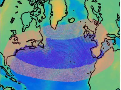
The second main idea of this thesis is that of spatially deforming a solution to a stochastic partial differential equation. In this way, a random field with a needed degree of non-stationarity and anisotropy can be acquired. A coupled system of two such stochastic partial dif-ferential equations is used to model the joint distribution of significant wave heights and wave periods in the north Atlantic. The model is used to assess risks in naval logistics.
Keywords: Spatial statistics, Point processes, Substitute-CT, Gaussian ran-dom field, Stochastic partial differential equation, Significant wave height
Acknowledgements
I would like to thank my supervisor David Bolin for introducing me to the interesting field of spatial statistics and teaching me the SPDE-approach, since you are a leading expert in this field. When I studied for my master’s degree I could not choose between focusing on statistics or numerical solutions to PDEs, therefore I kind of did both. Due to the SPDE-approach I kind of did both for my PhD as well. I am also grateful for you finding the time when I have questions, and introducing me to interesting research topics.
I would also like to thank my co-supervisor Igor Rychlik for his great ideas and vast knowledge—your insights in ocean wave modeling and its effect on naval vessels have been an invaluable contribution to this thesis. Jonas Wallin for your ideas and quick comprehension of new problems as well as collabora-tion on Paper I and II. Jun Yu for your hospitality during my visit to Ume˚a and collaboration on Paper I. Janine Illian for your expert insight in point process theory, the importance of interdisciplinary work, and collaboration on Paper II.
A grateful thanks to Milo Viviani and Efthymios Karatzas for our friend-ship and fantastic jam sessions with 3lele. Thank you to all of you in the lunch group for making the days at the office much better. During these years I discovered, unexpectedly, how fun it is to teach. I would like to thank the people who have supported me in this, most notably Johan Tykesson, Reimond Emanuelsson, and Johan Jonasson.
Attending conferences has given me an important understanding of con-temporary ideas and modern tools in my area of research. These visits would not have been possible without the travel grants I was awarded. Therefore I would like to thank Wilhelm och Martina Lundgrens vetenskapsfond, Stif-telsen GS Magnussons fond, ˚AForsk, SVeFUM, and Oscar Ekmans stipendie-fond.
I would like to thank all my friends and family for being who you are, caring for me, and making life enjoyable. A particular thanks to Herman Lundgren for proofreading this thesis. Last, but certainly not least, I would like to thank Karin Mellqvist for all the strong support when I needed it.
Anders Hildeman Gothenburg, April, 2019
Paper I A. Hildeman, D. Bolin, J. Wallin, A. Johansson, T. Nyholm, T. Asklund, and J. Yu.
Whole-brain substitute CT generation using Markov random field mixture models.
Preprint
Paper II A. Hildeman, D. Bolin, J. Wallin, J. Illian. Level set Cox processes.
Spatial Statistics, 28: 169-193, doi:10.1016/j.spasta.2018.03.004
Paper III A. Hildeman, D. Bolin, I. Rychlik
Spatial modeling of significant wave height using stochastic par-tial differenpar-tial equations.
Preprint
Paper IV A. Hildeman, D. Bolin, I. Rychlik
Joint spatial modeling of significant wave height and wave period using the SPDE approach.
Preprint
My contribution to the appended papers:
Paper I: I participated in the development of the model. I conducted the analysis and drafted the manuscript by myself and, after consul-tation, produced the final manuscript. I co-developed the code together with J. Wallin and D. Bolin.
Paper II: I co-developed the model together with the other authors of the paper. I developed the code and conducted the analysis. I pro-duced the theoretical results of Appendices A and B together with J. Wallin and D. Bolin. I drafted the manuscript and we finalized it together.
Paper III: I co-developed the model together with the other authors and I produced most of the theoretical results. I developed the code and conducted the analysis. I drafted the manuscript and we finalized it together.
Paper IV: I co-developed the model together with the other authors. I pro-duced the theoretical results. I developed the code and conducted the analysis. All authors wrote the paper together.
Publications not included in this thesis:
• O. Eliasdottir,A. Hildeman, M. Longfils, O. Nerman, J.Lycke. A nationwide survey of the influence of month of birth on the risk of developing multiple sclerosis in Sweden and Iceland.
Journal of Neurology (2018), 265 (1): 108-114. doi:10.1007/s00415-017-8665-y
• O. Andersen,A. Hildeman, M. Longfils, H. Tedeholm, B. Skoog, W. Tian, J. Zhong, S. Ekholm, L. Novakova, B. Runmarker, O. Nerman, S.E. Maier.
Diffusion tensor imaging in multiple sclerosis at different final outcomes. Acta Neurologica Scandinavica (2018), 137 (2): 165-173. doi:10.1111/ane.12797
CDF Cumulative Distribution Function CSR Complete Spatial Randomness CT Computed Tomography EM Expectation Maximization EMG EM-Gradient
FEM Finite Element Method GMM Gaussian Mixture Model GRF Gaussian Random Field
Hs Significant wave height
INLA Integrated Nested Laplace Approximation LGCP Log Gaussian Cox Process
LHS Left Hand Side LSCP Level Set Cox Process
MALA Metropolis Adjusted Langevin Algorithm MC Monte Carlo
MCMC Markov Chain Monte Carlo MH Metropolis Hastings ML Maximum Likelihood
MRI Magnetic Resonance Imaging NIG Normal Inverse Gaussian PC Penalized Complexity PDE Partial Differential Equation PDF Probability Distribution Function PET Positron Emission Tomography RHS Right Hand Side
SDE Stochastic Differential Equation SPDE Stochastic Partial Differential Equation
T1 Mean wave period
Tp Peak wave period
Tz Mean zero-level crossing wave period
Contents
I Introduction 1
1 Introduction 2
2 Random fields 7
2.1 Spatially continuous random fields . . . 10 2.2 Spatially discrete random fields . . . 14 2.3 Spatial mixture models . . . 17
3 Spatial point processes 21
3.1 The Poisson process . . . 22 3.2 Cox processes . . . 24 3.3 Characterizations of point processes . . . 24
4 Stochastic differential equations 29
4.1 Partial differential equations . . . 31 4.2 Finite element method . . . 33 4.3 The SPDE approach to Mat´ern fields . . . 35
5 Estimation and inference 38
5.1 Maximum likelihood estimation using the EMG algorithm . . . . 39 5.2 Bayesian inference . . . 40 5.3 Monte Carlo simulation . . . 41
6 Applications 47
6.1 Computed tomography . . . 47 6.2 Magnetic resonance imaging . . . 48
7.1 Paper I: whole-brain substitute CT generation using Markov ran-dom field mixture models . . . 57 7.2 Paper II: Level set Cox processes . . . 59 7.3 Paper III: Spatial modeling of significant wave height using SPDEs 62 7.4 Paper IV: Joint spatial modeling of significant wave height and
wave period using SPDEs . . . 64
8 Future work 67
8.1 Future work related to Paper I . . . 67 8.2 Future work related to Paper II . . . 68 8.3 Future work related to Paper III and IV . . . 69
Bibliography 70
II Papers 74
Part I
Introduction
Introduction
The thesis you are currently holding in your hand (or reading in the soothing light of your screen) is a work made up of four articles in the field of spatial statistics. In order to set the stage for presenting this work you need to know the background and main concepts on which the effort was based. The remainder of this chapter is devoted to a brief introduction to the field of spatial statistics. Chapter 2 introduces the important concept of random fields, Chapter 3 introduces the basics of spatial point processes, and Chapter 4 introduces the basics of stochastic partial differential equations. The main philosophy behind the parameter estimation and statistical inference methods used are explained in Chapter 5. The models presented in this thesis were developed to solve problems arising in several separated fields of study. These fields have their own methods, technology, and nomenclature. Chapter 6 give an overview of the most important problems and concepts associated to the particular applications considered in this thesis. Chapter 7 presents brief summaries of the papers and finally, Chapter 8 discusses possible future extensions to the work of this thesis.
Spatial statistics is a subfield of statistics that arose from problems in the industrial sectors in the early 1800s. The purpose of spatial statistics is to draw conclusions or aid in decision making based on observed spatial data. The word spatial here referring to data that can be compared using geometrical concepts such as distance, direction, and/or neighborhood struc-ture. The methodology originated from the fields of forestry, agriculture, and mining (Gelfand et al., 2010).
In agriculture the yield of cereal was being studied. It was recognized that spatial variations in yield could be attributed partly to soil constituents or
3
other known covariates. The remaining variation usually showed some spatial dependency that needed to be accounted for.
In forestry, the distribution of trees was being studied. Spatially repulsive effects, such as the competition for sunlight and other resources, explained why trees did not grow infinitely dense. At the same time, spatially attractive effects due to pollination paths and seed dispersal explained why trees did not grow far apart from each other. In order to model the distribution of trees, such effects had to be represented by models and inference needed to be drawn based on data.
In mining, engineers needed to predict the prevalence of certain minerals in the ground based on samples. The samples were typically acquired by drilling holes in the ground. Sampling was costly and they needed as much information as possible from the smallest possible sample sizes.
The main philosophy behind the methodology of spatial statistics can be summed up in Tobler’s first law of geography, i.e., “everything is related to everything else, but near things are more related than distant things” (Tobler, 1970, p.236). Therefore, the methods are concerned with quantifying and modeling spatial dependency structures. Spatial data can be sorted into three main categories:
• Data sampled on a continuous spatial domain.
Between any two pointss1 ands2, in some continuous space, D, there are an infinite number of other points. The data consist of values at some of these points. The interest of the analyst is how these measure-ments relate to the values on the entire spatial domain made up of an uncountable number of locations. Examples of such data are surface air temperatures and water salinity.
• Data sampled on a discrete spatial domain.
The spatial domain only has a countable number of points. The data consist of values at some of these points. Example of such data sets are observed values associated with spatial regions such as countries, digi-tal images (that are made up of a discrete set of pixels), experimendigi-tal designs with “blocked” regions. For data on a discrete spatial domain there is usually some logic to the discretization that is not directly as-sociated to geometrical distances. The discretization might instead be due to regions of varying natural resources, policies, or risks. Hence, it is often of more interest to measure proximity using the neighbor-hood structure and number of paths between two locations instead of the typical metrics of geometrical distance.
• Spatial point pattern data.
For point patterns, the location of events are studied. The spatial do-main concerned is most often continuous. The big difference compared to the two other types of data is that the randomness is not in the values at the locations but in which locations were chosen. That is, the data is a countable collection of points; spread out over a (usually) continuous spatial region. Typical examples of point patterns are locations of trees in a forest, locations of robberies in a city, or locations of earthquakes in a geographical region.
Statistical analysis of spatial data is typically needed to answer one or more of the following questions:
• What are the values at unobserved points in space? (Spatial prediction / Kriging / interpolation)
• What are the parameter values of the spatial model explaining the data? (Model estimation)
• Is the assumed model reasonable? (Model validation)
Spatial prediction refers to prediction of values at unobserved points in space given the values at some observed ones, i.e., interpolation/extrapolation. Spa-tial prediction was of interest to the South African mining engineer Danie Ger-hardus Krige who pioneered research in this field. In spatial statistics such conditional prediction problems are hence, as a homage to Krige, referred to as Kriging. Often predictions are more than just point values, instead the analyst wants to know the whole conditional distribution given the observed data. From conditional distributions, important point estimates such as the expected value, median, or mode can be acquired. Additionally, estimates of the uncertainty such as the standard deviation or interquartile range can be acquired from the conditional distribution and give important information about the prediction error of the corresponding point estimate.
Model estimation is the act of fitting the parameters of a model to the observed data. This is typically needed in order to draw conclusions about the underlying process that generated the spatial data. For instance, a parametric model representing tree growth in a forest might have a parameter representing the repulsive effect between trees. Estimation of this particular parameter gives information about the extent of the repulsive effect among this particular species of tree.
Model validation examines a model’s ability to explain the observed data. Since conclusions are drawn based on data and some model assumptions, it is
5
important to assess whether these assumptions are reasonable given observed data. Validating a model is an important part of accepting or rejecting a theory in any scientific field. Hence, having methodology to validate a spatial model is of great importance. Moreover, if the model does not explain the data well, the Kriging estimates and model estimation might not give any useful information.
In order to perform meaningful spatial analysis, some model of spatial de-pendency is assumed, either explicitly or implicitly. The assumed model is often simplistic in order to make model estimation reliable and computation-ally feasible. However, the true, but usucomputation-ally unknown, mechanism of spatial dependencies might not be so simple. Therefore, some degree of model mis-specification will often be present. An interesting phenomena is that a true but complex model can often be less useful than a simplification. This is because a simple model often has analytical expressions of important characteristics, easier interpretation of parameters, a lighter computational footprint, and can be estimated using smaller sample sizes and/or with greater robustness. Due to these issues, statistical modeling is a constant balancing act between what is possible and what is required. Closing this gap is one of the main aims of research in spatial statistics. Particularly, this thesis has focused on adding flexibility while keeping a low computational cost and robust estimates. An effort has also been made on developing models in which parameters are easily interpreted and convey a message; a property that is important in communi-cating research results, especially in interdisciplinary work.
The archetypal spatial model is the mixed effects generalized linear model. Here,Y(s) is an observable random variable associated to the spatial location s. The mean ofY is dependent on some covariates{Bj(s)}Kj=1as well as some spatially varying random effectX(s), i.e.,
EY(s){Bj(s)}Kj=1, X(s) =g−1 β0+ K X j=1 βjBj(s) +X(s) ,
The link function, g, adds an extra layer of flexibility since the conditional mean does only need to be a linear model after transformation.
What makes this model stand out compared to a typical generalized linear model is the spatially dependent random effect X(s). Typically, X is used to model unknown covariates and/or interactions between values at separate locations. The distribution ofY(s) given the conditional expectation models independent randomness between measurements at separate locations, typi-cally measurement noise.
Spatial variations can act on different scales. For instance, looking at crop yield, there might be large scale variations due to regions with different weather and there might be small scale variations due to the distance to some nearby stream. Often, it is not possible to model all scales of variability simultaneously. Therefore, depending on the scope of the problem, the short scale variability might be included in the spatially independent noise of Y|X, or the long scale variability in the baselineβ0.
Chapter 2
Random fields
In statistics, conclusions are drawn based on incomplete information using concepts from probability theory. Probability theory concerns processes where the outcome of an action is not determinstic, i.e., the same action can result in different outcomes under exactly the same surrounding conditions. We will call such an action anexperiment and the outcome of the experiment a realization. A real-valued random variable is a mapping between a realization and a real value, i.e., X : Ω → R, where X is the random variable, X(ω) a
real value,ω∈Ω a realization, and Ω is the set of all possible realizations. A random field is a mapping between a realization and a, possibly infinite, set of random variables, X(s, ω), indexed in space. Heresdenotes a point in the spatial domain D.
Intuitively, we can think of a realization of a random field as a real-valued function in D. Hence, a random field is a random function with the domain
D. An example of two different realizations of the same random field on a bounded and continuous domain inR2can be seen in Figure 2.1. Note how the
two images show similar qualities even though they are, pointwise, completely different.
A random field can have a discrete spatial domain, or a continuous spatial domain. We will refer to a random field on a spatially discrete domain as a spatially discrete random field and the contrary as a spatially continuous random field. Likewise, the image of the random variables,X(s), (all possible values attainable) at a point s can also be continuous or discrete. We will refer to a random field where X(s) can only take on a countable number of values for any fixeds as a discrete random field. From here on we omit the dependence on the sample space in the notation, i.e., X(s, ω) = X(s).
Figure 2.1: Two realizations of the same stationary Gaussian random field on a bounded domain inR2.
As was mentioned in Chapter 1, spatial statistics concerns analysis of data observed on a spatial domain. For the case of the first two types of data (continuous- and discrete-domain spatial data), the quantity of interest is the values at points in space. In other words, the data can be seen as observations (or partial observations) of realizations of random fields. Also in the third type of data (spatial point patterns) a realization is often dependent on some underlying random fields, see Section 3. Therefore, the concept of random fields is a vital part of spatial statistical methodology.
Two important functions used to characterize random fields are themean function andcovariance function.
Definition 2.0.1 (Mean function). The mean function, µ(s), of a random field, X(s), is defined as
µ(s) :=E[X(s)].
Definition 2.0.2(Covariance function). The covariance function,Cov(s1,s2), of a random field, X(s), is defined as
Cov(s1,s2) :=E[X(s1)X(s2)]−µ(s1)µ(s2).
The mean function is afirst order characteristicsince it only concerns the behavior ofX at one location inDat a time. The covariance function instead relates the value at two locations with each other and is hence a second order characteristic.
An important concept of random fields isstationarity.
Definition 2.0.3(Strongly stationary random field). LetX be a random field on the spatial domain D. Furthermore, assume that translations are defined on D, i.e.,s2=s1+t.
9
The random field,X, is strongly stationary if the vector[X(s1), ..., X(sn)]
is equal in distribution to the vector[X(s1+t), ..., X(sn+t)]for any finite n,
any set of locations, and for any translation,t, that keep the locations within the spatial domain, D.
In other words, strong stationarity is when the joint distribution between a set of points is only dependent on their relative positions and not on their absolute positions. Random fields that are stationary have important useful properties. However, stationarity is a strong restriction and many real world problems can not be modeled by truly stationary random fields. However, for a small region the most random fields are approximately stationary.
A slightly less restrictive and related property of a random field is that of weak stationarity, also known assecond order stationarity.
Definition 2.0.4(Weakly stationary random field). A random field is weakly stationary if
Cov(s1,s2) = Cov(s1+t,s2+t), andµ(s1) =µ,∀s1,s2∈ D.
A strongly stationary random field with finite variance is weakly stationary. A weakly stationary field do not, however, need to be strongly stationary.
Just as stationarity concerns translations,isotropy concerns rotations.
Definition 2.0.5 (Isotropic random field). The random field is isotropic if [X(s1), ..., X(sn)] is equal in distribution to[X(r s1), ..., X(r sn)]for any
ro-tation,r, any finiten, and any set of locations.
An important property of a random field that is both weakly stationary and isotropic is that it will have a covariance function that only depends on the distance between the two points considered.
Another property of a random field that is of great concern both in Pa-per I and PaPa-pers III and IV is the Markov proPa-perty. There are three slightly different definitions of the Markov property, the local, global, and pairwise (Rue and Held, 2005). We here only present the global Markov property since it can be defined both for spatially discrete and spatially continuous random fields.
Definition 2.0.6 (Global Markov property). X is globally Markov if X(A) and X(B) are independent conditioned on X(C) for any two subdomains
A, B ⊂ D separated by a domain C ⊂ D. That is, if the values at points inA and the values at points inB are independent conditioned on the values of all points inC.
This implies that if we want to predict values ofXat locations inAand we know the values ofXat all locations inC, there is no additional information in knowing the values at locations inB. For many applications this is a natural property arising from the propagation of information in the physical system that is being modeled. However, the Markov property can be computationally beneficial and making a Markov approximation of a non-Markov system can— if done properly—be very attractive. This is a major part of both Paper I and Papers III and IV.
2.1
Spatially continuous random fields
A spatially continuous random field is a random field on D for which D is a continuous spatial domain. Typically D is a Riemannian manifold and in most applications of spatial statistics just some subset of R2 orR3.
An important theorem applicable to weakly stationary random fields on
Rd isBochners theorem (Stein, 1999).
Theorem 2.1.1 (Bochners theorem). A complex-valued function C(s),s ∈
Rd is a covariance function for a weakly stationary mean square continuous
complex-valued random field if and only if it can be represented as
C(s) = Z
eiω·sdF(ω),
where F is a positive finite measure.
The theorem states that the covariance function is related to a spectral measure, F, through a Fourier transform. Hence, it is possible to model co-variance structures using spectral methods. WhenF is absolutely continuous with respect to the Lebesgue measure, the Radon-Nikodym derivative of F
with respect to the Lebesgue measure exists and is known as thespectral den-sity. Often the spectral density can have an expression that is easier to work with than the covariance function. It might also be computationally advan-tageous to generate or analyze data using the spectral density. This is used frequently in ocean wave modeling and is of importance to Paper III and IV, see Section 6.3.
2.1.1
Gaussian random fields
A Gaussian random field (GRF) is a random field such that any finite set of points on the spatial domain has a joint Gaussian distribution. A mul-tivariate Gaussian distribution can be characterized by the mean value and
2.1. Spatially continuous random fields 11
covariance matrix. Likewise, a GRF can be characterized solely by the mean-and covariance-functions. Often it is easier to work with a centered GRF, i.e.,
µ(s)≡0. Such a field can easily be attained by subtracting the mean func-tion from the original random field. Since the dependency structure of a GRF is completely determined by the covariance function, a stationary covariance function will lead to a stationary GRF (if the GRF is centered).
2.1.2
Mat´
ern covariance
In applications, the amount of data and computing power is limited. A robust estimate of an arbitrary covariance function cannot be achieved since data is finite while the degrees of freedom of arbitrary covariance functions are in-finite. Therefore it is common to assume that the covariance function is of some parametric family with only a small number of parameters. One such popular parametric class of stationary and isotropic covariance functions is the Mat´ern class (Mat´ern, 1986; Stein, 1999). This class can be parametrized by the marginal variance σ2, a smoothness parameter ν, and a correlation dampening parameter, κ. The smoothness parameter,ν, controls the differ-entiability of the covariance function at the origin. For a Gaussian random field this controls the smoothness of the realizations of the field itself in the sense that the field is almost surely H¨older continuous with ν as the corre-sponding H¨older constant. Let r be the practical correlation range of the random field, i.e., the distance between two points for which their correlation is 0.1. Then the dampening, κ, is proportional to the inverse ofr,κ∝r−1. Increasingκmakes points a fixed distance apart less correlated while decreas-ingκhas the opposite effect. A good approximation is that√8ν/κcorrespond to the distance between points for which the correlation is 0.13. The marginal variance,σ2, is the variance of the marginal distribution ofX(s) for any fixed s∈ D.
The Mat´ern covariance function is very popular in spatial statistics due to its flexibility using only three easily interpretable parameters. Both the exponential and Gaussian covariance functions are special cases of it and Stein (1999) famously proclaimed ”Use the Mat´ern model“ due to its ability to model the local smoothness of a Gaussian random fields using theνparameter. The Mat´ern covariance function is defined as
C(h) =
σ2
2ν−1Γ(ν)(κh)
νK
ν(κh),
whereh=ks2−s1k, Γ is the gamma function, andKis the modified Bessel function of the second kind. The spectral density of the Mat´ern covariance
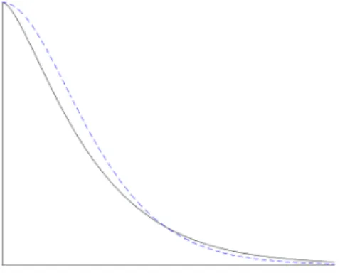
Figure 2.2: A Mat´ern covariance function as function of distance forν = 1 (solid line) andν = 2 (dashed line).
function is
γ(ω) =σ2Γ(ν+d/2)
Γ(ν)πd/2
κ2ν
(κ2+ω2)ν+d/2, where dis the dimensionality of the spatial domain.
In Figure 2.2 a Mat´ern covariance function is plotted for two different values of ν but with the same dampening and marginal variance. As can be seen, a larger smoothness parameter increases correlation for points close to each other but decreases correlation for points far away.
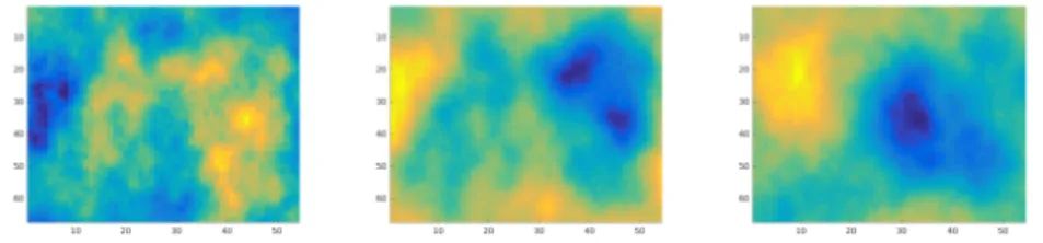
In Figure 2.3 realizations of three different Mat´ern Gaussian random fields can be seen. Notice the difference when changing the correlation range as well as when changing the smoothness parameter.
2.1.3
Gaussian white noise
A concept of great importance to this thesis is that of Wiener noise. In its most general definition it can be defined as follows (Adler and Taylor, 2007).
Definition 2.1.2 (Wiener noise). Let (D,A, ν) be a σ-finite measure space andA, B∈ A. Then, a Wiener noise satisfies
1. W(A)∼N(0, ν(A))
2.1. Spatially continuous random fields 13
Figure 2.3: Realizations of three distinctively different Mat´ern fields. Left:
ν = 1, r= 0.2. Middle: ν= 2, r= 0.2, Right: ν = 2, r= 0.4.
3. A∩B =∅ ⇒W(A)and W(B)are independent.
The measure space (D,A, ν) is for most practical considerations a subset of Rd with associated Borel σ-algebra and Lebesgue measure or the corre-sponding measure space when mapping this to a Riemannian manifold. As can be noted, the Wiener noise is a random measure on D with a centered normal distribution for which the variance is equal to the spatial measure of the subset chosen. Also, the covariance betweenW(A) andW(B) is equal to the spatial measure of the intersection A∩B. Since the Wiener measure of disjoint subsets of D has zero correlation, the Wiener measure of two small balls arbitrarily close but disjoint inDmust be independent of each other.
An alternative interpretation of the Wiener noise is as the Radon-Nikodym derivative of W with respect toν. With this interpretation,W is a random field. However, this random field do not have pointwise meaning and should be interpreted in a distributional sense, i.e., as a generalized random field (Stein, 1999).
As a generalized random field, the Wiener noise is defined by how func-tionals act on it. Considering the typical setting of a L2-space on D for which a functional,f(W), is defined through Riesz representation theorem as
hf, WiL2(D), the functionals with respect to a Wiener noise have the properties
f(W)∼N 0, Z D f(s)dν(s) E[f(W)g(W)] =hf, giL2(D).
In short, the Wiener noise is defined by how it acts on square integrable function on D. The usage of the Wiener noise in this thesis will be closely connected to a Gaussian random field with a Mat´ern covariance function. This connection is revealed in Chapter 4. Any Gaussian random field can be
generated as a convolution between the square root of the covariance function and a Wiener noise. This is used in Paper II to efficiently sample from a Gaussian random field using the method of Lang and Potthoff (2011).
2.2
Spatially discrete random fields
Spatially discrete random fields only have a countable number of spatial lo-cations in D. Such a space occurs either in applications where the space is inherently discrete or where the space has been discretized for some reason. In Paper I we consider a spatial domain that in reality is continuously indexed. However, the data are measurements of activity over regions rather than at points. Hence, the measurements need to be modeled on a discrete spatial domain.
2.2.1
Gibbs random fields
For a spatially discrete random field, the spatial domain can be expressed as an undirected graph, i.e., a set of nodes and edges between neighboring nodes. For an undirected graph, a clique is a set of nodes that are all neighbors of each other. A maximal clique is a clique which cannot be made any larger without losing the clique property. A specific class of discrete random fields are the Gibbs random fields.
Definition 2.2.1(Gibbs random field). Any probability distribution of values at nodes on an undirected graph defined as
P(X =x)∝e− P
c∈CEc(xc) (2.1)
is a Gibbs random field.
Here,C is the set of all maximal cliques andEc is a strictly positive
func-tion representing the energy associated with the configurafunc-tion of the cliques (Murphy, 2012, Chapter 19). The higher the energy in the clique, the less likely it is to occur. The proportionality constant of the Gibbs distribution will be denoted as W and is known as the partition function. The partition function is simply the sum of the right hand side of Equation (2.1) over all possible clique configurations. A Gibbs random field might involve a large number of nodes and hence a very large number of possible configurations. This often makes the partition function infeasible to compute.
2.2. Spatially discrete random fields 15
The Hammersley-Clifford theorem is an important result that relates Gibbs random fields to Markov random fields. We here recite the theorem as stated in (Winkler, 2003).
Theorem 2.2.2 (Hammersley-Clifford). Let a neighborhood system, N, on
D be given. Then the following holds:
1. A random field is a Markov field with respect to N if and only if it is a Gibbs field forN.
2. For a Markov random field, X with neighborhood systemN,
P(X(s) =x(s),s∈A|X(t) =x(t),∀t∈ D \A)
=P(X(s) =x(s),s∈A|X(t) =x(t),∀t∈ N(A)),
for every subsetA ofD.
A neighborhood system, N, here refers to a collection of sets such that s∈ N/ (s) ands∈ N(t) if and only ift∈ N(s) (Winkler, 2003).
The Hammersley-Clifford theorem states that all Gibbs random fields are equivalent to a Markov random field (MRF) and vice versa. Through the Hammersley-Clifford theorem a Gibbs field can be defined by conditional prob-abilities. Since neighborhoods usually involve a smaller number of nodes, the normalizing constant of such conditional distributions is often attainable al-though the partition function of the corresponding Gibbs distribution is not. In Paper I a Gibbs random field is used. This random field was defined by the conditional probability on the form
P(Xi =k|X−i) =
exp(−αk−βkfik(X−i))
W(α,β,X−i)
,
where fil denotes the number of points in the neighborhood of node i that
have the value l. The value ofXi can be referred to as the class that node i
belongs to. Theβ-parameters control the amount of attraction/repulsion be-tween points of classes. The α-parameters control the marginal probabilities of classes, i.e., they are equivalent but not identical with the, unconditional, probability of Xi belonging to a certain class. The three dimensional
neigh-borhood structure used in Paper I can be seen in Figure 2.4. In this paper, the spatial domain of the discretely indexed random field was on a lattice grid. In the figure, the white ball denotes a point at nodei. The black balls correspond to the first order neighborhood of node i, that is the points that have the smallest euclidean distance tosi on the lattice.
Figure 2.4: A first order neighborhood structure on a regular lattice in three dimensions.
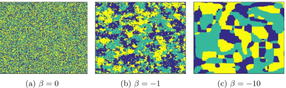
(a)β= 0 (b)β=−1 (c)β=−10
Figure 2.5: Example of realizations of a 3-class Potts field using three different values of the attraction parameter.
Figure 2.5 shows three realizations of such a random field on a two di-mensional lattice having three different classes (here illustrated by the colors blue, green, and yellow). The first figure was generated without any spatial interaction, βk = 0, the second with an attractive effect, βk = 1, and the
third with an even stronger attractive effect,βk= 10. As can be seen, theβk
parameters control the average size of the class regions.
2.2.2
Gaussian Markov random fields
A Gaussian random field on a discretely indexed domain can be stated as a multivariate Gaussian distribution. For a Gaussian random field on a fi-nite spatial domain this distribution can be characterized by the probability
2.3. Spatial mixture models 17 density function f(x) = |Σ| −1/2 (2π)n/2e −1 2(x−µ) TΣ−1(x−µ) .
Here, µ is the mean vector whose elements denotes the mean value for each of thenpoints inD. The corresponding covariance matrix between each pair of points in D is denoted by Σ. The inverse of the covariance matrix, i.e., the precision matrixQ= Σ−1, explains the conditional dependence between points in the Gaussian random field.
The PDF of the Gaussian random field has similarities with that of a Gibbs field, see Equation (2.1). In particular, ifQis non-zero only for pairs of points which are neighbors to each other, the Gaussian random field will be a Gibbs field. By the Hammersley-Clifford theorem it will hence be a Markov random field.
In spatial statistics, the computations that are of main concern when work-ing with a Gaussian distribution is computwork-ing the conditional mean, condi-tional variance, and likelihood. The computacondi-tional difficulties with these tasks can basically be reduced to evaluating the determinant ofQ, matrix multipli-cations with Q, and solving a linear system with Q. The precision matrices for non-degenerate Gaussian distributions are positive definite and symmet-ric. Hence, Qcan be factorized using the Cholesky decompositionQ=LLT
where Lis a lower triangular matrix. Having the precision matrix expressed by L is beneficial since solving a linear system of a triangular matrix has a computational complexity ofO(n2), as compared toO(n3) for general matri-ces. Also, the determinant equals the square of the product of the diagonals ofL. The only problem is that computing the Cholesky triangle,L, generally has a computational complexity ofO(n3).
Rue and Held (2005) made a strong point when showing that for a Gaussian Markov random field, the computational complexity of the Cholesky factoriza-tion is greatly reduced. Considering a spatial domain in two dimensions, the computational cost of the Cholesky factorization is reduced toO(n3/2) which makes a big difference when considering a spatial domain of many points. This property is one of the key benefits of the models proposed in Papers III and IV, see Section 4.3.
2.3
Spatial mixture models
A finite mixture model (Everitt and Hand, 1981) can be defined in two differ-ent but equivaldiffer-ent ways. Let us start by defining K classes; each associated
with a random variable Xk with corresponding probability distributionsDk.
Assume further a random variable, Z, with probability distribution D0, on a discrete sample space, {1,2, ..., K}. The K different values thatZ can as-sume correspond to theKclasses. The random variableY will be distributed according to a finite mixture model if it is generated by first acquiring a real-izationz fromZ, then assigningY the value from a realization ofXz. Hence
Y =
K
X
k=1
I(Z =k)Xk.
The finite mixture model can be viewed as a doubly stochastic model since it requires evaluation of random variables in two steps. If a probability density function (or probability mass function) exists, the mixture distribution can equivalently be defined by fY(x) = K X k=1 πkfk(x),
where fY is the PDF (or PMF) ofY,πk=P(Z=k), andfk is the PDF (or
PMF) of Xk.
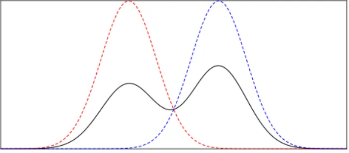
Typically, the first definition is used when the properties of the latent variable Z is of interest, which is the case for classification problems. The second definition is more common when a complex probability distribution should be approximated by a set of simple ones. For instance explaining a multimodal distribution as a superposition of unimodal ones as in Figure 2.6.
Figure 2.6: An example of a PDF for a finite mixture distribution (black) defined as the superposition of two Gaussian distributions (blue and red). The probability of being a member of the blue class is slightly larger than that of the red class, as can be seen by the right mode being larger.
2.3. Spatial mixture models 19
From here on out, finite mixture models will simply be referred to as mixture models.
In Papers I and II, mixture models were incorporated in spatial models where Z is no longer a random variable but instead a random field, Z(s). Likewise, {Xk}k are no longer random variables but random fields as well,
{Xk(s)}k. This is a natural extension of the mixture model definition to a
spatial model since the marginal distribution for a fixed point in space is a regular mixture model. Typically, such models can be used to classify regions of a spatial domain or to acquire non-linear prediction functions.
In Paper I, a spatial mixture model was used to model the distribution of voxel values in medical images. A Gibbs model was used to model the latent classification for each voxel. Given this classification, each voxel was assigned a value from the distribution of the corresponding class. Figure 7.2 shows an example of the classification of the spatial region into 4 different classes.
In Paper II, a spatial mixture model was used to model the distribution of the intensity function of a Cox process. The latent classification field, Z(s), was acquired from level sets of a Gaussian random field using the level set inversion approach of Iglesias et al. (2016) and Dunlop et al. (2016). Com-pared to the model of Paper I, this model has the advantage that it defines a classification field in a continuous spatial domain. In a geometric level set inversion problem,level set functions define a partition of the spatial domain through level sets of the function. That is, Ak ={s : ck−1 <X(s) ≤ck} ,
where {Ak}k is the partition and{ck}k are threshold values. The aim of the
inversion problem is to estimate the partitioning of the domain given obser-vations, Y(si) = K X k=1 akI(X(si)∈]ck−1, ck]) +i,
whereiare Gaussian i.i.d. random noise and ak are parameters.
Figure 2.7 show the observed field,Y, the underlying (latent) field,X, and the classification field,Z, acquired from thresholdingX in a realization of the level set model.
In Paper II, the Gaussian noise model of Dunlop et al. (2016) is replaced by a Poisson likelihood yielding an extension of the popular log-Gaussian Cox process.
10 20 30 40 50 60 5 10 15 20 25 30 (a) 10 20 30 40 50 60 5 10 15 20 25 30 (b) 10 20 30 40 50 60 5 10 15 20 25 30 (c)
Figure 2.7: (a) Observed data corrupted by noise,Y. (b) Corresponding level set function,X. (c) Classification field.
Chapter 3
Spatial point processes
A spatial point pattern is a countable set of locations, Y ={x1, x2, ...},xi∈
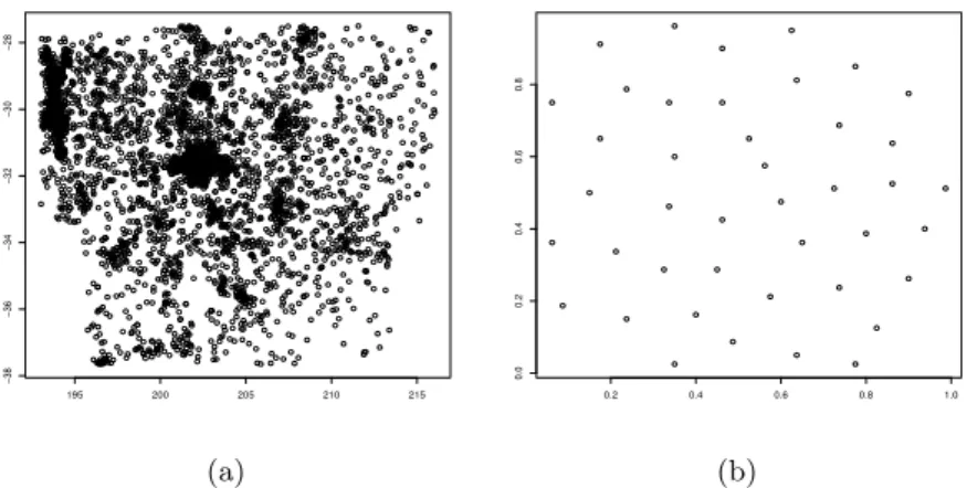
D on some continuous spatial domain, D. We can refer to the locations as events, in the sense that they correspond to locations where something occurs. Often the point pattern is observed in an observational window, W. That is, the point pattern exists on D but is only observed on W ⊆ D. Here, we consider two types of point patterns, the finite and the infinite. An infinite point pattern consist of an infinite number of events and is typically defined on an open domain such asRd. Practically, it is impossible to observe such a pattern in its full domain, i.e., the observational window will be a strict subset of D. A finite point pattern on the other hand will have a bounded spatial domain including all of the events. Practically, for a finite point pattern, the observational window is often the whole spatial domain while for an infinite point pattern, the observational window is never the whole spatial domain. Point patterns occur in a vast number of applications, e.g., locations of galaxies as seen in Figure 3.1a (Drinkwater et al., 2004; Baddeley and Turner, 2005), locations of cell centers observed under optical microscopy as seen in Figure 3.1b (Baddeley and Turner, 2005; Ripley, 1977), and location of trees as seen in Figure 7.3 and used in Paper II.
A point pattern can be defined as a counting measure,N, on the spatial domain D, where N(A) counts the number of points in the spatial region
A⊆ D. Often, point patterns can be seen as a realization from some stochastic model. Using the examples, whenever a new cell colony is grown, a new cluster of galaxies are observed, or a new region of forest is surveyed there will be a new point pattern observed. Of course, under similar conditions we expect
195 200 205 210 215 −38 −36 −34 −32 −30 −28 (a) 0.2 0.4 0.6 0.8 1.0 0.0 0.2 0.4 0.6 0.8 (b)
Figure 3.1: (a) Observations of galaxies in the Shapley supercluster. (b) Loca-tion of centres of observed biological cells observed under optical microscopy.
corresponding point patterns to have similar structures, even though the set of locations are different. Hence, we need to characterize the stochastic model from which the observed patterns emanated. A point process is a stochastic model of point patterns in the same way as a random variable is a stochastic model of real values. Since a point pattern could be described as a counting measure, a point process can be described as a random counting measure. Statistical analysis of point patterns corresponds to analyzing the properties of the point process that generated these point patterns.
3.1
The Poisson process
Historically, the most important point process is the homogeneous Poisson process. This is the model of complete spatial randomness (CSR), i.e., an unstructured point pattern. That is, events occur independently of each other and the number of points in a chosen region are distributed according to a Poisson random variable with intensity parameter proportional to the spatial measure of the chosen region. In this work, we will only consider spatial domains in euclidean spaces with corresponding Lebesgue measure, L, i.e,
E[N(A)]∝ L(A), whereA⊆ D, andDis the spatial domain. This definition
yields that the point process for CSR is defined by a random counting measure
3.1. The Poisson process 23
Historically, most methods in point process statistics have focused on dif-ferentiating between CSR and structured patterns. A structured pattern can either differ from CSR due to interaction between points and/or by spatial dependencies due to some available or unknown covariates. The difference between the two effects lies in the generative process more than the actual observed pattern. For example, assume that a seed is planted in a spatial re-gion. The seed grows into a tree and then a new seed is planted. If the second seed is planted too close to the first tree, the plant will be shaded. The shade inhibits its possibility of growing into a large tree itself. This is an example of a repulsive interaction between points. On the other hand, the possibility of the plant growing into a large tree might also depend on the topography and soil constituents of the spatial region. Planting a seed close to a stream or in a dry desert will affect its chances as well. This is an example of spatial dependency.
Definition 3.1.1 (Intensity measure). The intensity measure, Λ, of a point process is a deterministic measure defined as the expected value of the random counting measure, i.e.,
Λ(A) =E[N(A)], A∈ D.
If Λ is absolutely continuous with respect to the spatial measure, it can be described by the intensity function λ as Λ(A) = R
Aλ(s)ds. For the
ho-mogeneous Poisson process, λ(s) =λ,∀s∈ D, i.e., a constant intensity. The inhomogeneous Poisson process is a point process which behaves as a homoge-neous Poisson process on infinitesimal subregions ofD. Due to the additivity of Poisson distributed random variables, the counting measure of an inhomo-geneous Poisson process is Poisson distributed as N(A)∼P ois(Λ(A)). Any Poisson process (homogeneous or not) is characterized solely by the intensity measure, Λ.
The inhomogeneous Poisson process can model some types of spatial de-pendencies. If an intensity function exists, covariates can be included in the model by letting λbe a function of the covariate values. In Paper II, a log-linear relationship is considered where logλ(s) = P
jBj(s)βj for covariates
Bj and coefficientsβj. However, the inhomogeneous Poisson process assumes
no interaction between points, a feature inherited from the CSR model due to the additivity of Poisson random variables. Hence, it is an important but restricted special case of point processes.
3.2
Cox processes
A further extension of the Poisson process is that to a Cox process. In this process, λ(s) is itself modeled as a random object, i.e., a positive random field onD. Conditioned on a given realization ofλ(s), the point process is an inhomogeneous Poisson process with λ as its intensity function. Hence, the model is doubly stochastic in the sense that it defines a generative process based on two steps of random objects. A Cox process can also be considered as a Bayesian model of a Poisson process, where the latent intensity field,λ, is given a prior probability distribution.
A popular Cox process model is thelog-Gaussian Cox process (LGCP) for which λ(s) = eX(s), and X is a Gaussian random field. The popularity of the LGCP model is partly due to the marriage between the two most used and studied spatial stochastic processes, the Gaussian random fields and the Poisson processes. The popularity of the LGCP is also partly due to its versatility. It can model point patterns under uncertainty about covariates, i.e., it is unknown how and which covariates that affect the probability of events. The uncertainty about the covariates is explained by the randomness of λ. It can also model clustering effects, i.e., attractive interaction effects. Regions with higher intensity inλwould correspond to clustered regions with a higher probability of observing many events. The structure of the random field,X, could in this sense explain to what extent points tend to be clustered. A Cox process is however not enough to characterize all point processes. For instance, repulsive interaction effects such as trees competing over sunlight cannot be explained by such a model.
3.3
Characterizations of point processes
Just as moments, PDF’s, and CDF’s characterize a random variable, point processes can be characterized by some similar concepts. One such character-ization is through the moment measures. The moment measures characterize the k-th order moments of N(A), analogously to how the intensity measure was defined.
Definition 3.3.1 (k-th moment measure). The k-th moment measure of a spatial point process is defined as
µ(k)(A1×...×Ak) =E[N(A1)...N(Ak)].
3.3. Characterizations of point processes 25
Note that Λ(A) =µ(1)(A), the first order moment measure does not char-acterize interactions but higher order moments do.
Just as with random fields, the concepts of stationarity and isotropy are defined for point processeses.
Definition 3.3.2(Stationarity). A point process with counting measureN(A) is said to be stationary if,
P(N(A1) =n1, ..., N(Ak) =nk) =P(N(B1) =n1, ..., N(Bk) =nk),
for any finite set {Al}kl=1 where Bl = Al+t = {s : s−t ∈ Al}, i.e., a
translation of Al. (Illian et al., 2008)
Definition 3.3.3 (Isotropy). A point process is isotropic if,
P(N(A1) =n1, ..., N(Ak) =nk) =P(N(B1) =n1, ..., N(Bk) =nk),
for any finite set {Al}kl=1 where Bl = {s : Rθs ∈ Al}, i.e. a rotation with
angleθ of the points ofAl around the origin. (Illian et al., 2008)
The concept of ergodicity is also an important one. For an ergodic point process, the dependency betweenN(A) andN(B) will be negligible if the clos-est points in the two regions are sufficiently far away. This property means that if an ergodic point pattern is observed on a sufficiently large observational window,W, subregions far away from each other will have points distributed as if from different realizations of the underlying point process. The impli-cations being that, as long as the observational window is large enough and the point process is ergodic and stationary, one point pattern is enough for statistical analysis of the underlying process—since it acts as having observed several independent realizations of point patterns from the same point pro-cess. Historically, point pattern data have been scarse and spatial statisticians have often been forced to work with single replicates of point patterns. To draw any conclusion from such a dataset the ergodicity property is necessary. Nowadays, more often datasets have an abundance of replicates and ergodicity becomes less important.
A point pattern is a set of countable point locations in a sample space of uncountable point locations. For analysis, it can often be of interest to consider probability distributions conditioned on one or more events at spe-cific locations. This shifts the viewpoint from “an absolute frame of reference outside the process under study, to a frame of reference inside the process” (Daley and Vere-Jones, 2003). Such probabilities can be modeled using Palm
distributions. The Palm distribution of a point process is a probability distri-bution of point locations conditioned on that one of the points of a realization is located at a location,o. We will denote the expectation with respect to the Palm distribution as Eo, in contrast to the regular expectation with regards
to the absolute frame of reference, E. The following definition holds for a
stationary point process.
Definition 3.3.4 (Palm expectation).
Eo[f(Y)] = 1 λL(W)E " X x∈Y∩W f(Y −x) # ,
whereY is a point process,W is the observational window, andf is some real valued function of a point pattern. (Illian et al., 2008)
In words, the Palm expectation gives the expected value of f(Y) condi-tioned on that one of the points of realizations are observed ino.
In point process literature, some functional characteristics have been given particular attention. Here, a functional characteristic refers to a function that characterizes some aspect of the point process. Originally they were mainly used to test if point patterns behaved as CSR. Nowadays they are commonly used also to evaluate the goodness-of-fit of more general point process models, i.e., compare if the estimate of the characteristic from an observed point pat-tern is similar to that of the model. In Paper II, a point patpat-tern is compared to simulations from several assumed models. Evaluation of the model’s per-formance is based on the similarity of the functional characteristics between the real pattern and the simulated ones.
In the case of a stationary point process, Ripley’s K-function (Ripley, 1977) (or estimates thereof) has been used extensively in order to investigate departures from complete spatial randomness.
Definition 3.3.5(Ripley’sK-function). For a stationary and isotropic point process with counting measure N(A), the K-function is defined as,
K(r) = 1
λEo[N(b(o, r)\ {o})],
where b(o, r)is the ball with center in point oand radiusr.
In words,K(r) is the expected number of other points found inside a ball of radius rnormalized with the intensity and conditioned on that there is a point in the center of the ball. For the CSR model,K(r) =bdrd, where bd is
3.3. Characterizations of point processes 27
the volume of the unit ball inRd anddis the spatial dimension of the point
pattern. Hence, by estimating the K-function from the point pattern, it is possible to study the deviations from the theoretical K-function of the CSR model. For a point process with attractive spatial interaction (clustering),
K(r) > bdrd. Likewise, a point process with repulsive spatial interaction
(regularization),K(r)< bdrd.
A variant of the K-function that represents the same information but is easier to interpret is Besag’sL-function (Ripley, 1977, Besags comments),
L(r) = K(r)
bd
1/d
.
TheL-function is a modification ofK such that for the CSR model, L(r) =
r and estimations tend to be homoscedastic with respect to r. A further modification asL∗(r) =L(r)−rtransforms theL-function into the centered L-function for which the CSR model would haveL∗(r)≡0.
The pair correlation function, g(r), is another functional characteristic which also relates to theK-function by,
g(r) = K 0(r)
dbdrd−1r
,
whereK0denotes the derivative ofK. For the CSR model,g(r)≡1. Values of
g(r) larger than 1 means that there is a clustering effect at distance,r, while
g(r) < 1 means that there is a repelling effect. Typically, a point process might have attractive effects on some intervals and repulsive effects on others. Taking the example with tree locations, a repulsive effect exists for points very close to each other due to the competition for sun. However, at medium distances there should be an attractive effect since the seed dispersal has a limited range.
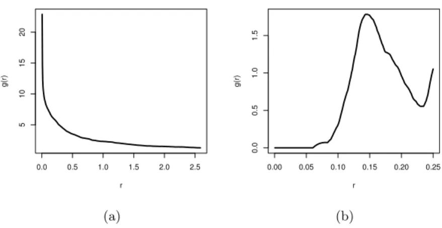
Figure 3.2 shows estimates of the pair correlation function for the two point patterns shown in Figure 3.1. The galaxy dataset show a clustering effect on short distances seen by g(r) > 1, while the cell data seem to be regularly spaced, seen by the peak above 1 at the range of 0.11−0.20. This fits intuitively with the visual perception of the two point patterns seen in Figure 3.1.
In the setting of Paper II, we have used estimates of the pair correlation function in order to compare our point pattern with simulations from the fitted models. In that setting, we did neither assume isotropy nor stationarity of the point process. However, we still expect the fitted model to yield estimated functions similar to the ones estimated from the actual point pattern. Hence,
0.0 0.5 1.0 1.5 2.0 2.5 5 10 15 20 r g(r) (a) 0.00 0.05 0.10 0.15 0.20 0.25 0.0 0.5 1.0 1.5 r g(r) (b)
Figure 3.2: Estimated pair correlation functions. (a) Estimated g for the Shapley galaxy supercluster. (b) Estimated gfor the cell data.
even though the interpretation of the functional characteristics is not clear in the non-stationary case, estimates can still be used for comparison. For details about estimating the functional characteristics mentioned above, see Illian et al. (2008).
Chapter 4
Stochastic differential
equations
LetX(t) be a differentiable function defined on the interval [0, T] andµ(x, t) a function ofxandt. If
dX(t)
dt =µ(X(t), t), X(0) =x0,∀t∈[0, T],
then X(t) is a solution to an ordinary differential equation (ODE) of first order with the initial value condition X(0) = x0. ODEs often describe the evolution in time of a variable given some initial condition, i.e. a temporal system. Since this thesis concerns models for spatial statistics, we can also considerX(t) to be a function in one-dimensional space, not necessarily time. In real world applications there is often some type of random noise present. This noise can be due to measurement errors in equipment used to gather data or uncertainties about the exact domain of the study. There can also be some stochasticity inherent to the actual system of study. For an ODE, this randomness leads to the solution,X(t), being a stochastic process rather than a deterministic function. This random behavior can be modeled by considering the differential to be a function of some random process, i.e.,
dX(t) =µ(X(t), t)dt+σ(X(t), t)dB(t). (4.1) Here, dB(t) denotes a random process (or generalized random process) and
σ denotes a function characterizing the influence of dB(t). Such a differen-tial equation with a random component is known as a stochastic differential equation (SDE).
The solution to equation (4.1), when such exist, is no longer a deterministic function but a stochastic process itself. SDEs provide an alternative way of characterizing a stochastic process, as compared to, e.g., autocorrelation functions and spectral densities.
The solution to a SDE can be interpreted in several ways, the most intuitive being the strong solution.
Definition 4.0.1 (Strong solution to SDE). X(t)is a strong solution to the SDE of Equation(4.1)if the integralsRt
0µ(X(t), t)dtand Rt
0σ(X(t), t)dB(t) exists for all t∈[0, T] and
X(t) =X(0) + Z t 0 µ(X(t), t)dt+ Z t 0 σ(X(t), t)dB(t).
The stochastic integral Rt
0σ(X(t), t)dB(t) is an integral where the inte-grand is a stochastic process and which is integrated with respect to a stochas-tic measure induced by dB(t). Furthermore, integrating dB(t) with respect to σ≡1 gives rise to the stochastic processB(t) defined as
B(t) =B(s) + Z t
s
dB(t).
For an exact definition of a stochastic integral, see (Klebaner, 2012, Itˆo- and Stratonovich-calculus).
Often SDEs are defined with respect to a Brownian motion process, i.e.,B
is a Brownian motion. A Brownian motion has the property
B(t)−B(s)∼N(0, t−s), s≤t,
and is continuous everywhere but nowhere differentiable. Hence, dB(t) is defined as a Wiener noise in one dimension whenB(t) is a Brownian motion. Since the solution to a SDE is a stochastic process, X(t) is a random variable for any fixedt. The distribution ofX(t) for large fixedt:s is often of interest.
Definition 4.0.2 (Invariant probability distribution of stochastic process).
An SDE is said to have an invariant probability distribution, π, if X(s)∼π
implies that X(t)∼π,∀t > s.
Note, not all SDEs have an invariant probability distribution. One impor-tant SDE that does have one is
dX(t) = 1
4.1. Partial differential equations 31
where f(x) is a twice continuously differentiable PDF of a probability distri-bution. In fact, the invariant probability distribution of Equation (4.2) is the distribution characterized by the PDF f. That is, with any feasible initial value, the marginal distribution of X for time T will converge to a random variable with PDF f as T → ∞. This is utilized in the MCMC method MALA, see Section 5.3.1.
Often we cannot compute the solutions to the SDEs explicitly, instead we have to approximate them numerically. A common method used to acquire approximations of sample paths of SDEs is the Euler-Maruyama algorithm. It is the SDE equivalent to Eulers method (using Itˆo calculus).
Definition 4.0.3. Euler-Maryuama method
Consider a diffusion process such as in Equation(4.1). Decide time steps
ti:ti =ti−1+ ∆t, then
Xt+1=µ(Xt, t)∆t+σ(Xt, t)∆Bt,
where∆Bt D
=B(t+ 1)−B(t).
4.1
Partial differential equations
The ODE gave rise to a solution which was a function in one dimension. This is enough when considering the evolution of some value over time—spatial prob-lems on the other hand are often concerned with observational domains in two-or three-dimensions. Modeling spatial systems in dimensions higher than one can be achieved with differential equations that include differential operators with respect to several variables, i.e.,partial differential equations (PDE).
A PDE can be a differential equation in both spatial variables and time. It is common to make a distinction between these two classes of variables; since time is causal and spatial dimensions are not, i.e., spatial dimensions are acausal. In this thesis we are concerned with purely spatial PDEs with respect to the Laplacian and gradient operators. Most of all, we are interested in the stationary dampened heat equation,
κ2−∆X(s) =F(s),∀s∈ D,
with some boundary value conditions. Here,sdenotes a point in ad-dimensional space and ∆ is the Laplacian operator, i.e., ∆f(s) := Pd
i=1
∂2
∂s2
i
f(s). The boundary value conditions considered are typically: the value of X at the
boundary of D(Dirichlet), the value of the projection of∇X on to the nor-mal vector at the boundary (Neumann), or a mixture of the two (Robin).
This PDE models heat transfer in materials which are able to absorb heat to a certain degree. The RHS,F(s), is known as thesource termand models heat sources and heat sinks, κ2 models the dampening, where a large κ2 correspond to a material with a high degree of heat absorption.
The strong solution does not exist for all PDEs. This is often because the strong solution has to be a smooth function while abrupt changes in material constants or heat sources often occur in real world problems. However, in the physical world we often observe solutions to PDEs, even when the strong solution does not exist!
The problem is that the strong solution is interpreted pointwise, i.e., the partial differential equation should hold for every point in the spatial domain. In reality, this is not how the solution to most physical systems should be interpreted. Instead, the differential equation does not need to hold for every point but it should hold in a distributional sense, such a solution is known as the weak solution. We present the weak solution for the dampened heat equation on a subdomain D ⊆ Rd with respect to the Hilbert space L2(D) and its inner product h·,·i. First, assume that the strong solution,X, exists and is smooth enough such that
κ2−∆
X(s), φ
<∞ for some class of functions φ∈V. Then, by Green’s first identity,
κ2−∆X(s), φ=κ2X(s), φ+h−∆X(s), φi=κ2X(s), φ
+h∇X(s),∇φi − hn· ∇X(s), φiΓ =:a(X, φ),
whereh·,·iΓdenotes the inner product on the boundary ofD,n(s) the normal vector to the boundary at points∈∂D, andV is a function space of differen-tiable functions. Note thata(·,·) is a bilinear form, i.e., linear in both its first and second argument. The bilinear form describes the differential operator in a distributional sense. The weak solution to the PDE would beX ∈U which fulfills
a(X, φ) =hF, φi, ∀φ∈V. (4.3)
That is, the functionX(s) in the function space U for which the LHS equals the RHS for any choice of φ withinV. Here, U is known as the trial space and V as the test space. The choice of test- and trial spaces depends on a
and F, since both a(X, φ) andhF, φihas to be well defined and bounded for every choice of φ∈V andX ∈U. The boundary conditions can be incorpo-rated into the weak formulation, either by constraining the test space further
4.2. Finite element method 33
(for Dirichlet boundary conditions) or implicitly through a modification of the bilinear form (for Neumann boundary conditions). Note that if a strong solution exists it is also a weak solution.
We here considered the dampened heat equation since this will be of im-portance in Papers III and IV. For other PDEs the weak solution can be defined in a similar fashion where a(·,·), U,and V will depend on the PDE, the boundary conditions, and the spatial domain,D.
4.2
Finite element method
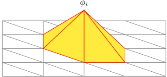
PDEs occur in many forms and on all kinds of spatial domains. Often, an explicit solution is not available. Instead, we are forced to resort to numerical methods to approximate the true solution. One class of numerical approxi-mations to solutions of PDEs are the finite element methods (FEM). These approximations are based on the weak formulation of the problem. The test-and trial spaces are in most problems infinite dimensional test-and therefore hard to handle practically. The Galerkin method can be used to reduce dimension-ality. Here, the test- and trial-spaces are reduced to the same finite dimen-sional subspace, i.e., Uh =Vh⊂V. In words, instead of forcing the equality
of Equation (4.3) to hold for all possible choices ofφ∈V, it is only required to hold for allφin a subspace,Vh. Also, the solution should be found within
the class of functions, Vh.
SinceVhis a finite dimensional space, the weak solution of Equation (4.3)
is reduced to a system of linear equations,
NU
X
i=1
zia(φi, φj) =hF, φji,∀j ∈ {1, ..., N} ⇔KZ=Fh. (4.4)
Here,{φi}Ni=1are basis functions ofVhand{zi}Ni=1are the coefficients yielding the approximate solution, Xh = P
N
i=1ziφi. The solution, Xh, exists and
is unique if a(·,·) is bounded, symmetric, and coercive and Vh is a closed
subspace of the Hilbert space considered (Brenner and Scott, 2008, theorem 2.5.6).
Obviously, the true solution will fulfill Equation (4.4) ifX∈Vh. IfX /∈Vh,
the approximate solution,Xh, will not be identical to X andkX−Xhk>0.
Galerkin’s method has an important orthogonality property,