Classification and Separation Techniques based on Fundamental Frequency for Speech Enhancement

(1)

UNIVERSIDAD DE JAÉN

ESCUELA POLITÉCNICA SUPERIOR

DE LINARES

DEPARTAMENTO DE INGENIERÍA

DE TELECOMUNICACIÓN

TESIS DOCTORAL

CLASSIFICATION AND SEPARATION

TECHNIQUES BASED ON FUNDAMENTAL

FREQUENCY FOR SPEECH ENHANCEMENT

PRESENTADA POR:

PABLO ANTONIO CABAÑAS MOLERO

DIRIGIDA POR:

DR. D. PEDRO VERA CANDEAS

DR. D. NICOLÁS RUIZ REYES

JAÉN, 11 DE ENERO DE 2016

(2)

Classification and Separation

Techniques based on Fundamental

Frequency for Speech Enhancement

Ph.D. Thesis

P

ABLO

A

NTONIO

C

ABAÑAS

M

OLERO

January 2016

Dept. of Telecommunication Engineering

University of Jaén

(3)

This work was carried out under the supervision of

Dr. Pedro Vera Candeas

Department of Telecommunication Engineering

University of Jaén

Linares, Jaén, Spain

Dr. Nicolás Ruiz Reyes

Department of Telecommunication Engineering

University of Jaén

(4)

Abstract

In the last decades, the fast development of digital signal processing technology has generated a growing interest on applications based on audio signals. Speech classification and separation algorithms are essential in this context because, in practical situations, the speech signal is degraded by background noise and other interferences, which is a serious obstacle for certain applications. In this thesis, we focus on the development of new classification and speech enhancement al-gorithms based, explicitly or implicitly, on the fundamental frequency (F0). The F0 of speech has a number of properties that enable speech discrimination from the remaining signals in the acoustic scene, either by defining F0-based signal features (for classification) or F0-based signal models (for separation).

In this thesis, we work in two different application scenarios. In the first one, it is assumed that the algorithms must be implemented on digital hearing aids which impose strong constrains in terms of computational capacity. We develop an acoustic environment classification algorithm based on F0 to classify the in-put signal into speech and nonspeech classes. The proposed pitch estimator is able to determine the F0 of the input signal with low computational cost, while maintaining a high speech/nonspeech classification accuracy. In addition, we also focus on the problem of classifying the input signal on a frame-by-frame basis for voiced speech detection, with the aim of developing a low-complexity speech enhancement algorithm based on F0.

In a second scenario, we assume that the aforementioned limitations no longer apply. In this case, we address the problem of speech and noise separation us-ing compositional models and source-specific mathematical constrains. In recent works, compositional modeling of audio with matrix decomposition algorithms, most of them derived fromnonnegative matrix factorization(NMF), has obtained very good results in audio source separation, specially in music signals. Although its application to speech has not been as explored as in music, the great potential of these techniques is very promising. The proposed signal model, in conjunc-tion with the developed regularized NMF, obtains better separaconjunc-tion measures for speech and noise separation than other NMF-based methods without the proposed restrictions.

(5)

(6)

Resumen

Durante las últimas décadas, el desarrollo de las tecnologías de procesado digital de señal ha despertado un interés cada vez mayor por las aplicaciones basadas en señales de audio. Los algoritmos de clasificación y separación de voz resultan esenciales en este contexto, puesto que, en situaciones prácticas, la señal vocal se encuentra afectada por ruido de fondo u otras interferencias, lo cual dificulta o impide ciertas aplicaciones. Con esta tesis se pretende dar lugar a nuevos algo-ritmos de clasificación y mejora de voz basados, explícita o implícitamente, en la frecuencia fundamental (F0). La F0 de la voz posee unas propiedades que per-miten la discriminación de esta fuente respecto al resto de señales de la escena acústica, ya sea mediante la definición de características (para clasificación) o la definición de modelos de señal (para separación).

En esta tesis se abordan dos escenarios de trabajo. En el primero, se supone que los algoritmos deben implementarse en audífonos digitales, con las enormes restricciones en capacidad computacional que ello conlleva. Se desarrolla un al-goritmo de clasificación de entorno acústico basado en F0 capaz de clasificar la señal en las clases voz y no-voz. El algoritmo propuesto consigue estimar la F0 de la señal utilizando un mínimo coste de recursos, sin alterar gravemente los re-sultados de la clasificación. En segundo lugar, se aborda también el problema de clasificar la señal de entrada trama a trama para la detección de voz sonora, con objeto de desarrollar un algoritmo de mejora de voz de bajo coste basado en F0.

En un segundo escenario, se supone que no existen restricciones graves de capacidad computacional. En este caso, se aborda el problema de la separación de voz y ruido mediante el uso de modelos basados en patrones, con restricciones específicas para voz y ruido. En la literatura reciente, modelos basados en pa-trones junto con algoritmos de descomposición de matrices, casi todos basados

ennonnegative matrix factorization(NMF), han obtenido muy buenos resultados

en separación de fuentes sonoras, sobre todo en música. Aunque su aplicación a señales de voz ha sido algo menos explorada, las posibilidades de estas técnicas resultan prometedoras. El modelo propuesto, junto con un algoritmo de descom-posición NMF con restricciones, permite separar voz y ruido obteniendo mejores resultados que otros modelos basados en patrones sin las restricciones propuestas.

(7)

(8)

Preface

This PhD thesis has been carried out at the Department of Telecommunication En-gineering, University of Jaén, and supported by the Andalusian Business, Science and Innovation Council under project 2010-TIC6762.

First, I wish to express my gratitude to Dr. Nicolás Ruiz Reyes, the person who encouraged me to start my research career on signal processing, and whose support, advice and expertise have been very valuable for me throughout these years. I also want to thank Dr. Pedro Vera Candeas for his excellent guidance, research attitude and kind cooperation during the course of my research work. Without his wide technical knowledge and ideas this thesis would not have been possible.

I am grateful to the members of the research group TIC-188, especially to Dr. Damián Martínez Muñoz and Dr. Francisco Jesús Cañadas Quesada for their numerous collaborations, and for giving me help and support when required. Also, I owe thanks to the people of the Multispeech group at INRIA Nancy, in particular Dr. Juan A. Morales Cordovilla, for the warm welcome and for giving me the opportunity to live an enriching experience.

Of course, I want to thank all the guys from the lab who have made my work-ing environment so friendly and enjoyable, includwork-ing Julio, Antonio, Rocío, Fran-cisco, David, Juan, Amparo, Pedro, José Guadalupe, Salah, Piedad, Diego, Casto, Violeta and Unai. A special mention belongs to Dr. Julio Carabias Orti and Dr. Francisco J. Rodríguez Serrano, whose simultaneous work has been very helpful, and who have been always around to share knowledge and code.

Finally, my deepest gratitude goes to my family, for their love and uncondi-tional support.

Pablo Antonio Cabañas Molero January 2016

(9)

(10)

List of Included Publications

This thesis is a compound thesis consisting of the following 3 publications, which are preceded by an introductory overview of the research field and a summary of the contributions. The publications are referred in the text with [P1], [P2] and [P3].

P1 P. Cabañas-Molero, N. Ruiz-Reyes, P. Vera-Candeas, and S. Maldonado-Bascon, “Low-complexity F0-based speech/nonspeech discrimination ap-proach for digital hearing aids”, inMultimedia Tools and Applications, Vol-ume 54, Issue 2, August 2011, pp. 291–319.

P2 P. Cabañas-Molero, D. Martínez-Muñoz, P. Vera-Candeas, N.

Ruiz-Reyes, and F. J. Rodríguez-Serrano, “Voicing detection based on adaptive aperiodicity thresholding for speech enhancement in non-stationary noise”,

inIET Signal Processing, Volume 8, Issue 2, April 2014, pp. 119–130.

P3 P. Cabañas-Molero, D. Martínez-Muñoz, P. Vera-Candeas, F. J. Cañadas-Quesada, and N. Ruiz-Reyes, “Compositional model for speech denois-ing based on source/filter speech representation and smoothness/sparseness noise constraints”, accepted for publication inSpeech Communication, Spe-cial Issue on Advances in Sparse Modeling and Low-rank Modeling for Speech Processing, 2015.

(15)

(16)

Chapter 1

Introduction

The design of machines that are able to “listen” has been one of the most attractive lines of research in the last years. Although human listeners are extraordinarily skilled in identifying and focusing on speech sounds, even in adverse acoustic conditions, these tasks are extremely challenging for machines. In real scenarios, the speech waveform observed by a listener is altered by multiple factors, includ-ing competinclud-ing sources, environmental noises or degradations introduced by the transmission channel. In these conditions, most of the speech processing knowl-edge acquired for clean speech is not enough for practical applications, and new techniques are required for handling degraded speech.

In this thesis, we are interested in developing classification and separation techniques that are useful for speech enhancement. We can define speech en-hancement asthe set of operations aiming to improve the quality and intelligibil-ity of the desired speech source, introducing some kind of technology between the

(possibly noisy) speech signal and the human listener. Nowadays, thanks to the

fast growth of digital systems, this technology for processing digital information is ubiquitous, but the solutions in this field still require intensive research.

There are a great number of applications where speech enhancement and clas-sification plays an important role. For example, in digital hearing aids, it is very useful to automatically classify the acoustic environment surrounding the user. When the presence of a speaker is detected, the device can activate a hearing pro-gram to improve the perception of speech. On the other hand, if the input signal is just noise, the device can select a more comfortable program, in order to avoid the amplification of annoying sounds. In hands-free communication systems, the signal reaching the microphone may suffer from a severe degradation, being not intelligible or annoying for the listener at the other side of the communication channel. Speech separation is also useful for restoring old or degraded record-ings, for example, in surveillance systems.

(17)

1.1

Speech and Fundamental Frequency

Although humans can produce a great variety of speech sounds, the shape of the vocal tract and its mode of excitation are restricted, which enables to find common properties to describe how speech is. Without necessarily knowing much about the speech production process, we can observe several basic characteristics of the speech signal by simply looking at a typical speech waveform, such as the one depicted in Figure1.1.

We observe that the speech signal • istime variant

• is quasi-periodic in some segments (at voiced regions), has a stochastic

spectral characterin other segments (at unvoiced regions) or ispaused • isquasi-stationaryin time intervals of 5-25 ms, which implies that the

vo-cal tract shape (and, consequently, its transfer function) remain nearly un-changed within this interval

• changescontinuously and gradually, not abruptly.

These characteristics of the speech signal are determined by its generation process, which originates in the lungs as the speaker exhales. Speech consists of pressure waves that are created by the airflow passing through the vocal tract. The vocal folds in the larynx can open and close quasi-periodically to interrupt this airflow, resulting invoiced speech. Vowels are the most prominent examples of this type of sound. Voiced speech is characterized by its periodicity, where the frequency of the excitation provided by the vocal chords is known as the

fun-damental frequency. The periodicity of voiced speech gives rise to a spectrum

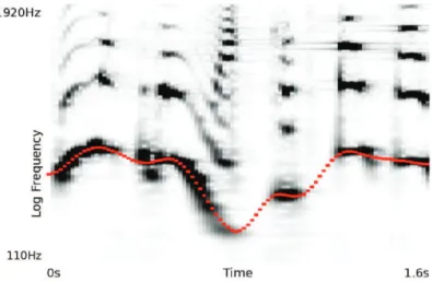
Voiced Unvoiced 120 80 40 0 ms

(18)

Figure 1.2:A speech spectrogram andF0contour.

containing harmonics at approximately multiples of the fundamental frequency f0, placed at frequencies lf0, for integers l ≥ 1. These harmonics are known

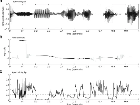
as partials. It is worth noting that voiced segments are not perfectly periodic, but locally quasi-periodic, which causes that the resulting spectrum is not purely harmonic. Forunvoiced speech, the vocal chords do not vibrate. Instead, the exci-tation is provided by a turbulent airflow passing through a constriction in the vocal tract, which gives to unvoiced phonemes a certain noisy characteristic. The posi-tions of the other articulators in the vocal tract serve to filter the noisy excitation, amplifying certain frequencies while attenuating others. The spectra for unvoiced speech usually have a more or less flat shape, with prominence of high frequency components.

In Figure1.2, we can observe more properties of the speech spectrogram and the fundamental frequency. As seen, the pitch produced by a speaker varies slowly across time, according to the speaker’s intonation. In addition, as a consequence of the alternation between voiced and unvoiced speech, the spectrum alternates har-monic regions with not periodic regions which do not produce harhar-monics. When the speech signal is corrupted by background noise, the speech spectrum still has spectral spikes that are strongly marked, while the spectrogram of the background noise has a tendency to be more flat, without significant spiky regions. Conse-quently, detecting the harmonic parts of the spectrogram in a noisy background can be viewed as searching for thin and harmonically distributed “islands” which rise out of a “sea” of noise [110].

Obviously, the harmonic structure of the spectrum is not exclusive to speech signals. Many other sounds, such as musical instruments, produce harmonics at multiples of a fundamental frequency. However, the evolution across time of

(19)

the pitch sequence is characteristic of speech, and presumably is a good cue for discriminating (and separating) speech from other sounds. Some psychoacoustic experiments demonstrate that the human auditory system employs the perceived pitch not only for discriminating the target source from inharmonic noises, but also from other harmonic interferences [25].

Consequently, when designing an algorithm for speech classification or sepa-ration, we can take the following points into account:

• The pitch contour and the voiced/unvoiced behavior of speech can provide useful features for speech classification.

• For speech separation, the employed speech model should have the typical harmonic structure of speech, and the background model should have a non-harmonic spectrogram or be prevented from having similar pitch evolution.

1.2

Scope of the Thesis

This thesis is focused on developing classification and separation algorithms for speech signals affected by background noise. We have employed the pitch proper-ties of speech signals to derive these algorithms. In this thesis, we intent to explore two application scenarios:

• Ultra-low power devices, such as hearing aids, with restricted computational capacity.

• Usual scenario without computational restrictions.

For both scenarios, we suppose that the background noise only contains envi-ronmental sounds, and not a competing speech signal. No further assumptions are made about the background noise or the speaker. The algorithms must work with one channel signals. We can formulate the following objectives:

• Develop a sound classification algorithm for hearing aids able to, at least, discriminate between speech and nonspeech classes, based on features ex-tracted from F0.

• Develop a frame-by-frame voicing detection algorithm to separate speech from background noise based on pitch and voicing decisions, and explore its implementation on hearing aids.

• Explore decomposition algorithms based on compositional models to create signal models for speech and background noise, with the aim of separating both signals.

(20)

1.3

Scientific Contributions

Main scientific contributions of the thesis comprise:

• Formulation of the decimated difference function for estimating F0 in ultra-low power devices, where the computational resources are very limited [P1]. • Definition of a dynamic threshold for the aperiodicity measure derived from the difference function, enabling to detect voiced segments with this feature in the presence of non-stationary noise [P2].

• Formulation of a compositional model based on mathematical constraints that represent the properties of background noise in a generic way, and are highly discriminative with respect to the typical shape and pitch evolution of speech [P3].

Three publications are included in this thesis, summarized in the following list. Chronological order of publishing is used.

[P1] Low-complexity F0-based Speech/Nonspeech Discrimination Approach for Digital Hearing Aids

As mentioned earlier, digital hearing aids impose strong complexity and mem-ory constraints on the development of signal processing algorithms, avoiding the application of conventional solutions. This paper proposes a low-complexity ap-proach for automatic speech/nonspeech classification in digital hearing aids, based on an efficient estimation of the fundamental frequency. The proposed scheme consists of two stages: analysis and classification. In the analysis stage, a set of signal features derived from F0 are computed. Here, F0 is estimated using a decimated version of the difference function, which considerably reduces the re-quired number of operation per second with respect to the conventional difference function. For the classification stage, two low-complexity classifiers are evalu-ated: the C4.5 decision tree and a Multi-layer Perceptron (MLP), the MLP being finally chosen because it provides the best classification accuracy rates and fits to the typical computational and memory constraints of hearing devices. Finally, a Hidden Markov Model (HMM) is used to provide some temporal context to the decision sequence. To demonstrate the feasibility of its implementation in a realistic hearing aid, the number of operations and memory requirements of the algorithm are analyzed, and compared to the computational capacity of a realistic processor for hearing aids. For the experiments, an audio database including clean speech, noisy speech, music and noise signals has been used.

(21)

[P2] Voicing Detection based on Adaptive Aperiodicity Thresholding for Speech Enhancement in Non-stationary Noise

In this study, we present a novel voicing detection algorithm that employs the well-known aperiodicity measure to detect voiced speech in signals contaminated with non-stationary noise. The method computes a signal-adaptive decision threshold which takes into account the current noise level, enabling voicing detection by direct comparison with the extracted aperiodicity. This adaptive threshold is up-dated at each frame by making a simple estimate of the current noise power, being thus adapted to fluctuating noise conditions. Once the aperiodicity is computed, the method only requires a small number of operations, and enables its imple-mentation in challenging devices (such as hearing aids) if the difference function is computed as proposed in [P1]. Evaluation over a database of speech sentences degraded by several types of noise reveals that the proposed voicing classifier is robust against different noises and signal-to-noise ratios. Additionally, to evaluate the applicability of the method for speech enhancement, a simple F0-based speech enhancement algorithm integrating the proposed classifier is implemented. The system is shown to achieve competitive results, in terms of objective measures, when compared with other well-known speech enhancement approaches.

[P3] Compositional Model for Speech Denoising based on Source/Filter Speech Representation and Smoothness/Sparseness Noise Constraints

This work presents a speech denoising algorithm based on a regularized non-negative matrix factorization (NMF), in which several constraints are defined to describe the background noise in a generic way. The observed spectrogram is decomposed into four signal contributions: the voiced speech source and three generic types of noise. The speech signal is represented by a source/filter model which captures only voiced speech, where the filter bases are trained on a database of individual phonemes (resulting in a small dictionary of phoneme envelopes) and the source bases are pitch-related excitation patterns. The three remaining terms represent the background noise as a sum of three different types of noise (smooth noise, impulsive noise and pitched noise), where each type of noise is characterized individually by imposing specific spectro-temporal constraints, based on sparseness and smoothness restrictions. The method was evaluated on the CHiME-3 development dataset and compared with conventional semi-supervised NMF with sparse activations. Our experiments show that, with a sim-ilar number of bases, source/filter modeling of speech in conjunction with the proposed noise constraints produces better separation results than sparse training of speech bases.

(22)

1.4

Organization of the Thesis

The rest of the thesis is organized as follows. Chapter 2 introduces some funda-mental concepts about audio classification, with special attention to classification problems involving speech signals for enhancement. Techniques for fundamental frequency estimation are also reviewed. Chapter 3 focuses on speech enhance-ment techniques, including algorithms based on matrix decomposition and com-positional models. Chapter 4 presents the conclusions of the work. Finally, the articles published during the development of this thesis are included.

(23)

(24)

Chapter 2

Speech Classification for

Enhancement Applications

2.1

Introduction

The general structure of an automatic sound classification system can be described with the block diagram depicted in Figure2.1. The basic idea is to categorize the input signal into one of a set of possible output classes, according to a predefined taxonomy. From the sound data, a number of relevant features are extracted which are then classified by some sort of classification algorithm. Possible classification errors may be corrected by an optional post-processing step, which also controls the transient behavior of the algorithm. As an output, a label describing the class of the signal is returned.

2 State of the Art in Sound Classification

2.1 Introduction

In this chapter, an overview is presented of the state of the art in sound classification. In the literature, many sound classification algorithms are described, but only few are designed for hearing instrument applications. Most of them are determined for other applications, such as multimedia, and are only able to classify subsets of the classes that are desired for hearing instruments, for example different music types, background noises or alarm signals.

The general structure of a sound classification system can be described with a block diagram, as it is shown in Figure 2.1. From the sound data, a number of characteristic features are extracted, which are then classified with some sort of pattern classifier. An optional post processing step may correct possible classification outliers and control the transient behavior of the algorithm. The output of the algorithms are the recognized sound classes.

Sound Feature Extraction Pattern Classifier Post Processing Classes

Figure 2.1: General block diagram of a sound classification system.

In the following, five currently known methods for sound classification in hearing instruments will be presented. Three of them are already exploited in commercial hearing instruments, the analysis of the amplitude statistics by Ludvigsen (1993), the classification based on temporal fluctuations and spectral form by Kates (1995) and further developed by Phonak (1999), and the analysis of the modulation spectrum (Ostendorf et al., 1997). The two other algorithms are also designed for hearing instruments, but not exploited so far (Feldbusch, 1998, and Nordqvist, 2000).

The feature extraction blocks of the three already exploited approaches will be evaluated and compared. It will be shown that they are related in that most of the features described in these algorithms represent the amplitude modulations in the signal, and that this enables the discrimination of speech signals from other sounds very well. A more detailed classification of the acoustic environment is however hardly possible with these approaches.

Finally, a review of other sound classification algorithms is given. This includes procedures Figure 2.1:Block diagram of an audio classification system.

The criterion upon which the signals are classified depends on the target ap-plication, which also determines other properties of the system, such as decision delay or computational complexity. For example, in a music database manager, it is useful to organize audio collections by music genre. For an audio coder, the optimal coding scheme can be selected if the system is able to identify the au-dio at the input as speech or music. In the context of speech signals, automatic speech recognition (ASR) can be viewed as a classification problem, in which the input waveform is converted into a sequence of lexical units. In this thesis, we are interested in classification problems that are, in some way, useful for speech

(25)

enhancement purposes. If the ultimate goal is to improve the speech signal per-ceived by a listener, a classification algorithm can help in the process by selecting the best enhancing approach at each moment or by setting certain parameters of the enhancer. The following problems show why sound classification is useful for speech enhancement.

Acoustic environment classification is a topic of great importance in digital hear-ing aids [2, 12, 99]. According to the classifier decision, the device can select the most appropriate amplification program to the detected acoustic environment, thus increasing the comfort level. For instance, suppose that the user is listening to a speaker in the presence or not of certain background noise, such as in a conference or when watching television. In this situation, the hearing aid should decide that it is worth amplifying the signal (for ex-ample, by selecting a “speech amplification program”) in order to help the user understand the message. On the contrary, if the user is embedded in a noisy place, such as a traffic jam, the device should switch off the am-plification program, thus avoiding to amplify unpleasant noises and saving battery life. Detecting more specific acoustic environments, such as “mu-sic”, “speech in noise”, “speech in quiet” or “speech in mu“mu-sic”, is useful when the device implements hearing programs targeted to those situations. Voice activity detection (VAD) stands for locating speech segments from a noisy

input. Clearly, for enhancement applications, VAD can be used for updat-ing noise models (from detected silence) and selectupdat-ing speech segments for further processing (possibly taking advantage of the acquired noise mod-els). Since other sources may be active at amplitudes comparable to tar-get speech, just observing the input signal activity does not suffice for ro-bust VAD. Consequently, VAD remains as a complex classification problem [142], specially if the noise is nonstationary or speech-like. VAD can be viewed as a particular case of acoustic environment classification, in which "speech" and "nonspeech" are the only considered options. One of the con-tributions of this thesis is the design of a speech/nonspeech discrimination system for hearing aids, based on features derived from fundamental fre-quency [P1].

Voicing detection is the process of determining speech segments produced by vi-bration of the vocal chords [1]. Unlike VAD, whose purpose is to determine the presence of speech, either voiced or unvoiced, voicing detection focuses only on voiced parts. Since voiced segments are more or less periodic, this problem is often associated with fundamental frequency estimation, al-though this is not always the case. Voiced detection is very useful for cer-tain enhancement approaches, specially for those involving binary masking

(26)

[65], comb filtering [20], harmonic tunneling [34] or sinusoidal synthesis [68]. In this thesis, we propose a voicing detection algorithm based on a single feature, the aperiodicity, whose computation is made robust against nonstationary background noise [P2].

Classification and enhancement of speech signals can be viewed as closely re-lated problems, in the sense that the solution of the former facilitates resolving the later, and vice versa. A perfect speech separation reduces the classification prob-lem to characterizing separated sources, whereas a perfect classification enables to accurately approximate separation parameters and source signal models.

2.2

Feature Extraction

2.2.1

Signal Analysis

Digital audio signals are generally recorded as time-domain pulse-code modu-lation (PCM) waveforms. In order to analyze the signal, the input waveform is broken into small (possibly overlapping) short-term frames, also calledanalysis

windows. The temporal resolution of the system can be characterized by two

parameters, frame length and frame shift. The former defines the duration of each frame. It is set to a value where the input can be assumed mostly station-ary, which for speech may stand for 20–64 milliseconds. For classification, short frame lengths (around 20–25 ms) are preferred for capturing rapid dynamics of speech, whereas longer frames (around 64 ms) are often used in signal enhance-ment, where slower transitions reduce audible artifacts from estimation errors. Frame shift is the amount of input time advanced before extracting a new frame, and is usually set to 50% or less of frame length. The difference of these two values isframe overlap.

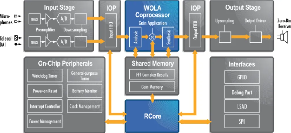
The input signal is usually transformed into a spectral domain, commonly by Fourier analysis of the short-term frames. Before computing the short-time Fourier transform (STFT), input frames are conventionally multiplied by a win-dow function (e.g. Hann or Hamming winwin-dow), in order to increase the sensitivity to weaker spectral components. The sequence of short-term spectra over time is called the spectrogram, denoted byX(t, f), where f is the frequency bin index and t is the time-frame index. Other usual frequency-time representations are obtained by filtering the time-domain signal with a filterbank of bandpass filters, such as in the weighted overlapp-add (WOLA) analysis [24], common in hear-ing aids, or the cochleagram [94], which is used for extracting auditory-based features.

(27)

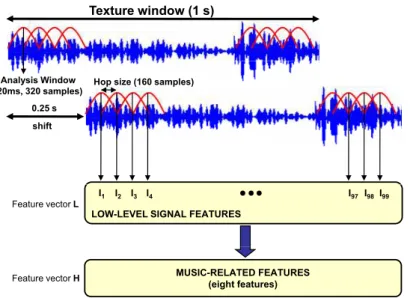
In the previous introductory discussion, we have assumed that a set of features, arranged as a feature vectorc, represents the object to be classified as a whole. De-pending on the portion of time represented by a feature vector, we can distinguish two different approaches: frame-based feature vectors andtexture-based feature

vectors. In the frame-based approach, a new feature vector is computed for each

frame or analysis window, hence representing the properties of the signal in por-tions of 20–64 ms, as mentioned above. The frame-based approach is useful when real-time classification is desired. However its major drawback is that it does not allow to take into account other long-term characteristics of the signal that often provide a better description of the different sound classes. While two signals, cor-responding to different classes, may appear similar in a single frame, observing their long-term behavior is more likely to bring out the characteristic patterns, en-abling a robust discrimination. As a result, the concept of texture window was introduced. A texture window is a long-term segment (in the range of seconds) containing a number of analysis windows. In the texture-based approach, only one feature vector for each texture window is generated. This feature vector is not just the concatenation of the vectors obtained in each frame, but often statistical measures of them, such as the mean or standard deviation. Also, certain features only have sense for long-term signal segments, and are often defined from fea-tures measured at each frame. For example, a feature describing properties of the pitch contour of a signal can only be computed for an extended observation pe-riod, based on consecutive frame-by-frame pitch estimations. When working with texture windows, the temporal resolution of the classifier is defined by thetexture

window lengthand thetexture window shiftparameters, both measured in number

of frames.

The texture-based approach is preferred in applications requiring an accurate classification, and where the decision can be returned with a certain delay. For instance, in the case of hearing aids, it is crucial to provide a robust and stable de-cision, even if the system takes a few seconds in reacting to environment changes [13,99].

2.2.2

Signal Features

In order to classify an incoming signal, some measures or featuresare extracted from it. A set ofDfeatures extracted from an analysis or texture window is rep-resented as a D-dimensional vector c = [c1, c2, . . . , cD]T called feature vector.

The key point is that the chosen features must contain valuable information that allows to properly distinguish among the considered classes. In other words, the features should measure signal properties that tend to present distinguishable val-ues among the different audio classes.

(28)

In classification of signals affected by noise, there are two approaches for extracting signal features. The first one consists in formulating features (or com-binations of features) that are robust to background noise, such that the signals pertaining to a certain class exhibit characteristic values for those features (or for their combination) in both clean and noisy conditions. The second one is based on performing some kind of preprocessing to estimate the effect of the noise before extracting the features, which are then redefined to take into account this effect. This preprocessing may be accomplished with noise estimation techniques (see Section 3.2.5). There is an obvious third approach consisting in enhancing the signal before extracting the features. However, in our study we are analyzing the classification problem as a tool for resolving signal enhancement and not the other way around.

Many signal features have been proposed in the literature for resolving the problems outlined in Section2.1. In the following, we overview some of the most common of these features.

Timbral Features

These features provide numerical quantities measuring the spectral shape of the signal. Probably, the most famous is the spectral centroid, defined in [115]. The spectral centroid of a short-term spectrum X(t, f) is a measure of the center of gravity of its energy distribution, and thus, it outlines if the spectrum contains a majority of high or low frequencies. Higher centroid values correspond to spec-tra skewed to the range of high frequencies. Due to its effectiveness to describe the spectral shape, the centroid has often been used in audio classification tasks in-cluding speech, noise and music classes [84,129]. A similar feature is thespectral

rolloff, defined as the frequency below which 85% of the accumulated magnitudes

of the spectrum is concentrated. This measured was first proposed as a feature to distinguish between voiced and unvoiced speech [115], since voiced frames tend to have a lower rolloff. It has also been found useful for discriminating speech from other sources, such as music [84]. Thespectral fluxis the average difference between the magnitude spectra corresponding to successive frames of the STFT. This feature is related to the amount of spectral local changes, being generally higher for speech than for noise or music [87]. Thevoice2whiteparameter, pro-posed in [54], is a measure of the energy inside the typical speech band (300–3600 Hz) with respect to the whole energy of the frame. Consequently, this feature is useful for discriminating between speech and nonspeech signals. Features such as the spectral flatness measure [66], theRenyi entropy [64] or theShannon

en-tropy [106] measure the degree of randomness in the signal, and hence are also

(29)

cross-ing ratecounts the number of times that the signal amplitude changes sign during the analysis window [129]. As with the previous features, it is also a measure of noisiness.

Auditory-based Features

The overwhelming majority of speech recognition systems today, as well as many classification algorithms, make use of features that are based on either Mel Fre-quency Cepstral Coefficients(MFCCs) [26] or features based onperceptual linear

predictive (PLP) analysis of speech [59]. MFCCs are a compact representation

of the spectrum of an audio signal that takes into account the nonlinear human perception of pitch. For the extraction of MFCCs, the FFT bins are combined according to a set of triangular weighting functions that approximate the human pitch perception as described by the Mel scale. This can be viewed as filtering the spectrum with a filterbank of triangular bandpass filters, and then integrating the output of each filter over the frequency. The filterbank usually consists of 40 filters, such that the 13 first filters (low frequencies, below 1 kHz) have linearly spaced center frequencies, and the 27 last filters (high frequencies, above 1 kHz) have logarithmically spaced center frequencies. The 40 filterbank output coeffi-cients are log compressed, an a Discrete Cosine Transform (DCT) is applied to decorrelate the coefficients, providing the so-called MFCCs. Usually, for classifi-cation tasks, only the first coefficients (between 5 and 20 MFCCs) are useful for obtaining a good performance. The cepstral computation can also be thought of as a means to separate the effects of the excitation and frequency-shaping compo-nents of the source-filter model of speech production.

The computation of the PLP coefficients is based on a somewhat different im-plementation of similar principles. As in MFCC processing, the input spectrum is weighted and integrated using a set of asymmetrical functions based of auditory perception. In this case, these functions are spaced according to the Bark scale, and are based on the auditory masking curves of [119]. The filter-bank output values are weighted by a preemphasis step to simulate the sensitivity of hearing (according to the equal-loudness curve), and the equalized values are raised to the power of 0.33. The resulting spectrum is processed by linear prediction to obtain a smoothed approximation based on all-pole modeling. Finally, cepstral coefficients are obtained from the predictor coefficients by a recursion that is equivalent to the logarithm of the all-pole model spectrum followed by an inverse Fourier trans-form. PLP processing is also frequently used in conjunction with the RASTA (relative spectral analysis) algorithm [60]. RASTA processing inserts a bandpass filter after the compressed values that emerge from the preemphasis step, in

(30)

or-der to model the tendency of the auditory periphery to emphasize the transient portions of incoming signals.

Theamplitude modulation spectrograms(AMS) are motivated by

neurophys-iological experiments on periodicity coding in the auditory cortex of mammals [127]. The AMS representation is a two-dimensional feature which contains in-formation about the prominent modulation frequencies for each center frequency. Each complex coefficient of the FFT is considered as a function of time across consecutive frames, i.e., as a band pass filtered complex time signal. The number of bands is reduced to a few channels (between 3 and 15) by adding the FFT coeffi-cients of neighboring bands, grouped according to a Bark scale. The signal in each band is analyzed again by computing the Fourier transform, producing a modu-lation spectrum for each channel. The modumodu-lation spectrum at each band is dis-cretized into a few coefficients following a logarithmic scale. For voiced speech, the AMS feature matrix exhibits vertical bars at the fundamental frequency and its multiples, being useful for speech and noise discrimination.

Other features inspired on Auditory Scene Analysis measure properties related to the onset/offset of sounds, frequency modulation, pitch or voicing [12]. Funda-mental frequency has a great potential for characterizing speech signals, because speech has a characteristic pitch behavior. Techniques for fundamental frequency estimation are reviewed in Section 2.4, along with the pitch-based features em-ployed in this thesis [P1] for speech/nonspeech discrimination in hearing aids. Other Features

Certain features describe the signal regarding its dynamic energy properties, its statistical behavior or its predictability [14]. Although the energy level of the sig-nal in a single frame is irrelevant for classification, its long-term variation can pro-vide useful information in distinguishing audio types. Several features have been proposed to describe the smoothed trajectory of the signal level, often extracted from texture windows. Some examples are the low energy rate, the evelope or the loudness. The statistical behavior of the signal can be described mathemati-cally by the central moments of its time-domain waveform, in features such as the sample skewnessor thesample kurtosis[14].

Another common feature in audio classification is derived from linear predic-tion analysis. A P-order linear prediction of a sample x(n) is a prediction of its amplitude value as a linear combination of its past P samples, in the form a1x(n −1) + a2x(n −2) +. . .+aPx(n −P). The ap coefficients are called

the Linear Prediction Coefficients(LPC), and can be obtained by one of several

algorithms proposed in the literature, which aim at obtaining a prediction error as lowest as possible. One of these algorithms is the so-called autocorrelation

(31)

method of autoregressive modeling [67]. The set of coefficients ap can be used

as a feature for classification, as well as the prediction error. Signals with sud-den amplitude changes and high noise components are more likely to yield higher values for the prediction error and vice versa.

Noise-adapted Features

A common approach in classification of signals degraded by noise is to redefine classic features taking into account the estimated noise level or the long-term be-havior of the features. Usually, the long-term bebe-havior of a feature is a good indication of its expected value in absence of speech. An example of this ap-proach is used in the G.729B standard [5], which conducts a VAD decision on every frame using four different parameters: a full-band energy difference, a low-band energy difference, a differential spectral flux measure and a zero-crossing rate difference. Essentially, these parameters are noise-adapted versions of classic features (full-band energy, low-band energy, spectral flux and zero-crossing rate) which are formulated as the difference between the parameter itself extracted in the current frame and its long-term average. The long-term averages of the param-eters are supposed to follow the changing nature of the background noise, and are updated based on a first order autoregressive scheme only if the full-band energy difference is less than a certain threshold.

A similar approach is applied in the ETSI advanced front-end (AFE) standard [38], but using the logarithmic energy (and its long-term estimated mean) as a unique feature. In this case, the VAD decision is based on a SNR threshold and a hangover mechanism that updates the mean logarithmic energy. A more elab-orate process is employed in the ETSI extended front-end standard [37]. Here, the algorithm maintains an estimate of the noise energy spectrum (defined on a mel frequency scale), and both a smoothed and long-term average version of the signal espectrum. At each frame, the algorithm computes the deviation between the smoothed signal spectrum and its long-term average, and the peak-to-average ratio in the smoothed signal spectrum. Whenever these quantities are below a threshold (which is an evidence of nonspeech), the noise spectrum is updated us-ing a smoothus-ing operator. The final feature for takus-ing the VAD decision is the estimated SNR. The algorithm also provides a voicing decision based on a pitch estimator, in which the presence of pitch is determined from a correlation score for each generated pitch candidate.

(32)

2.3

Classification Algorithms

After the feature extraction process, a decision on the class to which the input signal belongs to must be made based on the extracted features. This process is performed by the classifying algorithm. The extracted feature vector cforms the input to the classifier, and the output is the assignment of the input signal to one of theC considered audio classes, denoted aswk, withk = 1, . . . , C.

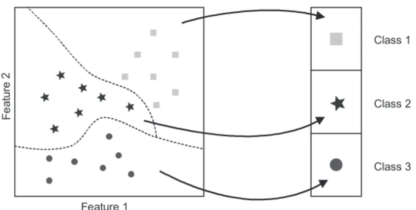
From a graphical point of view, classifying means to find in which decision region falls a given feature vector, and assigning to this vector the classwk

corre-sponding to the estimated region (see Figure2.2). The goal of pattern recognition is to use a set of available training samples to find decision boundaries that sepa-rate the classes in an optimal way. In other words, in atraining stage, the borders between classes that provide the best discrimination for a given set of training vec-tors (whose class is known) are found. Then, in thetest stage, the trained classifier can classify new unknown vectors according to the computed boundaries. Note that the training stage is performedoff-line, in a design phase, and not in the final application.

This intuitive idea of classification can be expressed more formally as follows: given a classification problem with C classes, a set ofC discriminant functions gk(c) is defined. Classification of a feature vector c consists of performing the

following operation:

Decidewiif gi(c)> gj(c) for allj 6=i. (2.1)

Thus, a classifier can be viewed as an algorithm that evaluates all discriminant functions for a given feature vector and assigns the class corresponding to the largest discriminant. The goal of the training phase is to derive this set of discrim-inant functions.

Depending on the chosen approach for finding these functions, classifiers can be grouped intogenerative classifiers andmachine learningclassifiers. The first ones model the probability density function (pdf) of the feature set for each audio class. In this case, classification can be interpreted as determining the probability of each class for a given input vector, and selecting the class that produces the highest probability. This type of classification algorithms include, among others classifiers, Hidden Markov Models (HMMs), Gaussian Mixture Models (GMMs) and, in general, all algorithms based on Bayesian classification. The advantage of these classifiers is that they are relatively easy to train because the pdfs of the feature set can be determined separately for each class. This training process in-volves estimating the parameters of the pdfs, which usually follow well-known and tractable mathematical expressions. For some algorithms, the pdf for cer-tain features are completely known (including their parameters), and no training

(33)

Feature 1 F e a tu re 2 Class 1 Class 2 Class 3

V

gure 6.2: Pattern classification viewed as establishing a mapping from feature space

Figure 2.2: Pattern classification viewed as establishing a mapping from a feature space

to a decision space.

is required. The major drawback of generative classifiers is, however, that they demand to know the probability distributions for the feature set a priori.

Machine learning classifiers, on the other hand, determine the boundaries be-tween classes without modeling the probabilities directly. Instead, they approxi-mate the discriminant functions by connecting a set of operations in series, where the parameters of these operations can be learned to achieve optimal class bound-aries. Examples of these classifiers include Artificial Neural Networks, Support Vector Machines or decision trees. Training this kind of algorithms can be a dif-ficult task because it involves considering all audio classes at the same time, and often demands the use of iterative algorithms which are not guaranteed to con-verge to a good result. On the other hand, discriminative classifiers can be very adequate when there is a large training set or a high number of features, and they are the only option when the underlying pdfs are unknown.

2.3.1

Generative Classifiers

Bayesian Classification

As mentioned above, the central problem in statistical pattern recognition is find-ing the set of discriminant functions for a classifier. TheBayes Decision Theory describes the classification problem when the pdfs of the classes are known. The pdf describing each class p(c_|wk) is the conditional pdf of cgiven the classwk.

This quantity is also called the likelihood of the observed vector when hypoth-esizing class wk. Besides, it should be noted that, in general, some classes in a

classification problem are more probable than others. Therefore, each class is also associated with itsa priori probabilityp(wk).

(34)

In order to make a classification, we want to know how probable a classwkis,

given an observationc. This is the so-calleda posteriori probabilityp(wk|c), and

its relationship to the class likelihood is provided by theBayes Rule: p(wk|c) =

p(c_|wk)p(wk)

p(c) , (2.2)

wherep(c) = PC_k₌₁p(c_|wk)p(wk). Consequently, for a given observationc, the

classifier will decide the class wk for which the posterior probability is highest,

thus obtaining the following decision rule:

Decidewiif p(wi|c)> p(wj|c) for allj 6=i. (2.3)

This decision rule is called the Maximum A Posteriori(MAP) criterion. Observe that the termp(c)is only a scale factor and does not affect the decision. Then, we can conclude that a MAP classifier is the one whose discriminant functions are given bygk(c) = p(wk|c).

In many problems, all classes are equally probable a priori. In this case, the p(wk)term is constant for allkand therefore it does not affect the decision. Thus,

with equal priors, maximizing the posterior probabilities is the same as maximiz-ing the likelihoods, obtainmaximiz-ing the followmaximiz-ing rule:

Decidewiif p(c|wi)> p(c|wj) for allj 6=i, (2.4)

which is called the Maximum Likelihood (ML) criterion. To decide a class for a given feature vector, we evaluate each conditional pdf and select the one that provides a higher value. The discriminant functions of a ML classifier aregk(c) =

p(c_|wk).

When the density forms of the classes are known, but their parameters are not, it is necessary to use aparameter estimationtechnique in a training stage, using a set of training feature vectors.

Gaussian Mixture Models

A Gaussian Mixture Model (GMM) represents the distribution of each class as a weighted sum of gaussian densities. Hence, each class wk can be modeled as a

mixture model, obtaining class likelihoods of the following form: p(c_|wk) =

M

X

m=1

akmpkm(c), (2.5)

where M is the number of gaussians andakm are the weights of each gaussian.

(35)

such thatpkm(c) ∼ N(µkm,Σkm), where each component within each class has

its own mean vectorµ_kmand covariance matrixΣ_km.

Training a GMM is done bymaximum likelihood(ML) parameter estimation, in which the set of parameters of the gaussians θk = {akm,µkm,Σkm} is

es-timated by maximizing the likelihood of a giving training set. Suppose that a training set consisting ofJ training samplescj is available for a given classwk.

ML estimation ofθkconsist of resolving the following problem:

ˆ θ_k= arg max θk J Y j=1 p(c_j_|wk,θk), (2.6)

where now we have written the class density asp(c_|wk,θk) to denote its

depen-dency of the set of parameters. Usually, this problem is accomplished by making use of a so-called expectation-maximization(EM) algorithm [28]. This consists of a set of iterations in which the parameters are updated in such a way that the the criterion in (2.6) increases monotonically until a certain threshold is reached. Hidden Markov Models

So far we have assumed that, given a single feature vector c, the system takes an immediate decision on the signal class. However, in many classification problems, it is necessary to observe a sequence of measurements through time,c0,c1, . . ., in

order to make a reliable decision. A clear example is seen in speech recognition, in which the decision about the word or phoneme pronounced by a speaker must be made after observing a sequence of vectors. In these cases, an audio class is not only defined by characteristic values of the feature vectors, but also by their progression through time. The most effective classifying tool for these situations is based on a structure referred to as Hidden Markov Models (HMM) [104].

HMMs are statistical models of time-series data. An HMM models a time series as having been generated by a process that goes through a series of states. Depending on the problem, each state may correspond to a different sound class or to a different phase within a certain sound class, in which case a different HMM is defined for each possible class. Suppose that the model hasQdifferent states, denoted as qi, withi= 1, . . . , Q. Given a feature vectorct, the likelihood of this

vector supposing that the model is in the stateqi at instanttisp(ct|qi,bi), where

bi is the set of parameters of the density function, and B = {b1,b2, . . . ,bQ}

is the global set of density parameters. The model is named hidden because the sequence of states is not observable, but only the visible feature vectors, which are supposed to be generated from the true sequence of states according to their corresponding density functions. When in any state, the next state that the process

(36)

State sequence Observation sequence

Figure 2.3: Schematic illustration of a HMM. The four circles represent the states of the

HMM and the arrows represent allowed transitions. Each HMM state is associated with a state output distribution as shown. The process progresses thorough a sequence of states. At each visited state, it generates an observation by drawing from the corresponding state output distribution.

will visit in the next time instant is determined stochastically, and is only depen-dent on the current state. The transition probability can be defined as the matrix A = _{aij}ij, whereaij is the probability of a transition from stateqi to stateqj.

Also, an initial state distributionπ =_{π1, π2, . . . , πQ}is defined, whereπi is the

probability that state qi is the first state in the state sequence. Graphically, the

progression of a HMM is represented in Figure2.3.

The compact notation λ = (A,B,π) is used to represent a HMM. The de-sign of a HMM for an audio class includes choosing the number of states Q as well as the density forms of the pdfs (e.g. GMMs), and estimate all the param-eters using a training set. The most common parameter estimation procedure is the Baum-Welch algorithm [71], based on expectation-maximization. In the test stage, given a sequence of vectorsc0,c1, . . ., all HMMs are evaluated to determine

their sequence of states, and the HMM (i.e. audio class) that produces the state sequence with higher probability is chosen.

HMMs can also be useful as a post-processing stage, in order to incorporate temporal information to the decision process. For example, each audio class can be represented by a different state, such that the resulting state sequence can be viewed as a smoothed decision sequence. In this case, the transition probabilities must be chosen carefully to determine the steadiness of the system.

2.3.2

Machine Learning Classifiers

k-Nearest Neighbor Classifier

The k-nearest neighbor classifier, or k-NN, is essentially a distance-based clas-sifier [32]. To obtain the class corresponding to a new vector c, the algorithm

(37)

simply looks for its k nearest vectors (neighbors) in the training set, and weigh, usually applying a majority rule, the class number they belong to.

For expressing this idea in a more formal way, let us consider a set ofJtraining samplescj organized intoCdifferent classes. The algorithm computes a distance

measure betweencand each vectorc_j in the training set, and selects theknearest cj. This distance criterion is often based on the Euclidean distance, so the

algo-rithm computes J distances as dj = ||c−cj||. The classifier assigns the label

which is most frequent among the k nearest samples (according to distancesdj).

Usually, choosing moderate values for k improves performance in comparison with choosing simply the class of the nearest vector, because it yields smoother decision boundaries and provides more probabilistic information. However, large values for k can be detrimental, not only because of the increased computation complexity, but because it destroys the locality of the estimation by considering samples that are too far away. In addition, from a computational point of view, a k-NN classifier requires to store all feature vectors of the training database in order to compare the input vector with each training instance. Consequently, if the classifier is implemented in a low-power device, such as a hearing aid, the number of training samplesJ must be very limited, as well as the value fork.

Artificial Neural Networks

An artificial neural network [62] is a parallel, distributed information processing structure consisting of a set of processing units, called neurons, interconnected via unidirectional links called connections. Each neuron has one or more inputs values and produces a single output which branches into one or more connections to feed other neurons. The mathematical operation performed within each neuron can be defined arbitrarily, with the restriction that it must be completely local; that is, it must depend only on the current input values arriving at the neuron and on values stored in the neuron’s local memory.

Among the multiple variations of neural networks, the most common is prob-ably the multilayer perceptron (MLP). The basic architecture of a multilayer per-ceptron consists of three layers of neurons (input, hidden and output layers) in which each neuron in the hidden and output layers is interconnected with all the neurons in the previous layer by links with adjustable weights. This type of neural networks is commonly known as “feed-forward neural networks”, and is probably the most popular and widely-used network in many practical implementations. It has the advantage that there are good training algorithms to determine the param-eters of the network, and the computational cost for classifying an input vector is moderate and deterministic. It is worth mentioning that multilayer perceptrons may have more than one hidden layer, but it has been shown that a single hidden

(38)

layer is sufficient enough to approximate any function to arbitrary accuracy, given a sufficient and finite number of neurons.

For a classification problem withC classes, in which the input feature vector c = [c1, c2, . . . , cD]T is composed of D features, the number of neurons in the

input layer is usually set to D, and the number of neurons in the output layer is set to C. With this configuration, each neuron in the input layer is fed by a single feature of the vector, and each neuron in the output layer produces the probability value for a single class. The number of neurons in the hidden layer M determines the complexity of the network, and must be designed carefully. If too many hidden neurons are used, the capability to generalize will be poor; on the contrary, if too few hidden neurons are considered, the training data cannot be learned satisfactorily.

As mentioned before, each neuron in the input layer is connected to all the neurons in the hidden layer, where each connection has an associated weight, denoted as adm, with d = 1, . . . , D and m = 1, . . . , M. The output value ym

produced by themth hidden neuron can be expressed as follows: ym =f D X d=1 cdadm+bm ! , (2.7)

wherebmis a parameter of the neuron andf(·)is the transfer function executed in

the neuron. This transfer function can take a variety of mathematical expressions, but the most common in MLPs is the logarithmic sigmoid, with the formf(x) = 1/(1+e−x₎_{. The output neurons perform the same processing that the one in (}_2.7_),

but they are fed by the valuesym produced by the hidden neurons, and connected

to them by links with their corresponding weights.

In the training process, the weights of the network and the parameters of each neuron are adjusted to approximate the desired function (i.e., to minimize the classification error for the given training set). A variety of algorithms has been proposed in the literature aiming at training multilayer perceptrons, including the gradient descent, Gauss-Newton or Levenberg-Marquardt [8].

In the last years,deep neural networks(DNNs) have rapidly gained popularity for resolving complex classification problems [63]. Proposed in 2006, DNNs en-able to approximate discriminative functions with a large number of features and training instances. Compared to the training methods of traditional deep mod-els with a high number of hidden layers, DNNs can prevent over-fitting to the training set via a special unsupervised pre-training procedure. Also, they can express highly variant functions, discover the underlying regularity of multiple features, and have strong generalization abilities. Recently, DNNs have received much attention in the speech processing community, with successful applications in speech recognition, natural language processing and classification [142].

(39)

2.4

Fundamental Frequency Estimation

A key property of many sounds, including speech and music, is the pitch. In the context of music, the American Standard Association defines the term pitch as that attribute of auditory sensation in terms of which sounds may be ordered on a scale extending from low to high [3]. As such, the pitch of a sound is strictly speaking a perceptual phenomenon, although it is caused by physical stimuli that exhibit a certain behavior. Signals that cause the sensation of pitch are, broadly speaking, that kind of signals that are well-described by a set of harmonically related sinusoids, meaning that their frequencies are approximately integer multi-ples of afundamental frequency. In fact, we can say that pitch is the perceptual correlate of the fundamental frequency of a signal, and is often described as “the perceived fundamental frequency of a sound”. In the literature, however, it is com-mon to use the terms pitch and fundamental frequency indistinctly, and we will do so throughout the text.

Signals that have frequencies that are integer multiples of a fundamental fre-quency can be represented using the following model forn = 0, . . . , N ₋1:

x(n) =

L

X

l=1

Alcos(ω0ln+φl). (2.8)

This signal model is often known as the harmonic model. The quantity ω0 is

the fundamental frequency and L is the number of harmonics, where the term harmonic refers to each sinusoid in the sum of (2.8). Al > 0andφl ∈ (−π, π)

are the amplitude and the phase of the lth harmonic, respectively. The amplitude determines how dominant (or loud) a given harmonic is, while the phase can be thought of as representing a time-shift of the harmonic, as we can express the argument of the cosine function as ω0ln +φl = ω0l(n − nl), with nl = _ωφ0ll.

The number of harmonics L can be any integer between 1 and π/ω0, although

it is generally not possible to say in advance how many harmonics are going to be present (in practice, however, it is assumed to be a known parameter). For mathematical convenience, it is more usual to formulate the harmonic model in terms of complex exponentials with the form ejw0ln. If the signal samples are

arranged into a vector x = [x(0), . . . , x(N ₋1)]T_{, and the complex amplitudes}

of the harmonicsAlejφl are grouped in vectora= [A1ejφ1, . . . , ALejφL]T, we can

write the harmonic model as

(40)

where Z is a matrix having a Vandermonde structure, being constructed fromL complex sinusoidal vectors as

Z=      1 1 _{· · ·} 1 ejw0 ejw02 · · · ejwL ... ... . .. ... ejw0(N−1) ejw02(N−1) · · · ejw0L(N−1)     . (2.10)

We recall that for signals that can be expressed using (2.8) or (2.9), the pitch, i.e., the perceptual phenomenon, and the fundamental frequency are the same. It is interesting to note that, while an harmonic signal is comprised as a sum of a number of individual components, these are perceived as being one object by the human auditory system.

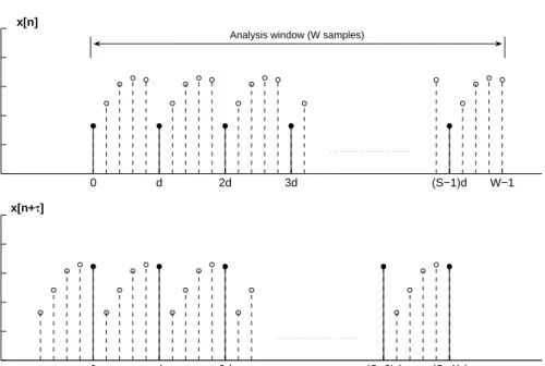
Functions that perfectly obey the harmonic model are periodic. In fact, any periodic signal can be decomposed using the model in (2.8) or (2.9). Periodic signals have the following property:

x(n) =x(n₋τ), (2.11)

or, equivalently, x(n) = x(n +τ), where τ is the so-called pitch period, i.e., the smallest time interval over which the signal x(n)repeats itself, measured in samples. It should be stressed that, while x(n)is defined for integersn, τ is not generally an integer. In fact, since pitch is a continuous phenomenon, it is not accurate to restrictτ to only integer values, although this is often done. The pitch period (in samples) and the pitchω0 are each others’ reciprocal, i.e.,ω0 = 2π/τ.

To express the fundamental frequency in Hz, denoted by f0, one must use the

relationω0 = 2πf0/fs, wherefsis the sampling frequency.

The signals generated by real-world sound sources are not strictly periodic; instead, their cycles are slightly different from each other, and hence we can say that practical signals are indeed pseudo-periodic signals. Additionally, in real-world sounds the harmonics do not perfectly match their theoretical values at in-teger multiples ofω0; instead, they depart somewhat from their ideal frequencies,

a phenomenon designated as inharmonicity. Also, in practical situations, the sig-nal is affected by background noise, and hence the model must take into account the presence of a stochastic, non predictable signal term. All these factors will affect our ability to always estimate the fundamental frequency correctly, and so the main challenge of a pitch estimator is to deal with these phenomena in a robust way.

Pitch estimation is then the art of findingω0 from an observed signal whose

characteristics are not known in detail, and where the signal may depart from pe-riodicity (or harmonicity) in several ways. Many pitch estimation algorithms have

(41)

been proposed in the literature. These may be divided into parametricand

non-parametric algorithms. While parametric algorithms assume an explicit model

for the noisy signal, for instance, the model in (2.8) for the source part, non-parametric methods do not make such assumptions. At this point, it is worth mentioning that the techniques reviewed here are limited to the single pitch case. In many situations, like in most music or multi-speaker recordings, the signal consists of many periodic sounds, in which case the signal is referred to as multi-pitch signal. In this thesis, we do not address problems involving the estimation of multiple fundamental frequencies, even though the model proposed in [P3] is potentially able to rep