Comparing the Performance of Alternative Generalised
Autoregressive Conditional Heteroskedasticity Models in
Modelling Nigeria Crude Oil Production Volatility Series
*A. E. Usoro, C. E. Awakessien and C. O. Omekara
Received 18 October 2019/Accepted 15 December 2019/Published online: 30 December 2019
Abstract There is no gainsaying the fact that crude oil production remains a major factor to the Nigeria economic growth given its significant contribution to the nation’s gross domestic product. Preponderance of the researches in the oil sector dwell more on oil prices, with less focus on the volatility of crude oil production. What cannot be overemphasized in oil sector is the production volatility effect which is mostly caused by unstable production quantity due to certain nation’s economic, social, political factors. In this paper, volatility of crude oil production was considered, and different Generalised Autoregressive Conditional Heteroskedasticity (GARCH) models were fitted to Nigeria crude oil production volatility series. Data for the work were monthly crude oil quantity data from January 2010 to August 2019 (NNPC ASB) from which the crude oil production volatility was measured. The suggested GARCH models included GARCH (0,1), GARCH (0,2), GARCH (1,1), GARCH (1,2), GARCH (2,1) and GARCH (2,2). Using Akaike Information Criterion (AIC), Bayesian Information Criterion (BIC) and Schwarz’s Information Criterion (SIC), GARCH (1,2) and GARCH(2,1) competed favourably. The MSE of forecast revealed GARCH (2,1) to perform better for the forecast of crude oil production volatility. Further findings will reveal other alternative models as the crude oil production pattern changes in the future.
Key Words: GARCH (p, q), GARCH (o, q),
volatility measure.
*A. E. Usoro
Department of Statistics, Akwa Ibom State University,
Mkpat Enin, Akwa Ibom State, Nigeria Email: [email protected] C. E. Awakessien
Department of Statistics, Michael Okpara University of Agriculture, Umudike, Abia State, Nigeria
C. O. Omekara
Department of Statistics, Michael Okpara University of Agriculture, Umudike, Abia State, Nigeria
1.0 Introduction
In univariate time series, a time dependent variable, say Xt may be characterised by linear, nonlinear or mixed process. Autoregresive (AR), Moving Average (MA) and Autoregressive Moving Average (ARMA) models are popular and commonly used in fitting stationary linear time series; (Box and Jenkins, 1976). The problem in the applications of AR, MA and ARMA is that they are not appropriate models for time series process described by large changes in variance at various time periods; (Franses, 1998). This is because the aforementioned models account for linear processes and cannot capture high variance properties of a series indexed at time t. The consistent change in variance over time may be increasing or decreasing, and this systematic change is called heteroskedasticity or volatility. Autoregressive Conditional Heteroskedasticity (ARCH) is a method that explicitly models the change in variance over time in a time series; (Engle, 1982). The ARCH model is considered suitable when the variance of the process or error variance in a time series follows an autoregressive (AR) process. If the variance is accounted for by autoregressive moving average (ARMA) process, the model is generalised autoregressive conditional heteroskedasticity (GARCH); (Bollerslev, 1986). The GARCH model is an extension of the ARCH model which considers autoregressive and moving average components of the process variance and error respectively. Originally, Autoregressive Conditional Heteroskedasticity is written in the form ARCH (q). The “q” is the order of the model, which indicates the number of lag errors as the predictor variables of the ARCH model. With the Generalised Autoregressive Conditional Heteroskedasticity, GARCH (p,q), “p” assumes
the order of the autoregressive component (the number of lags of the variance to be included as predictors), while “q” assumes the order of moving average component (the number of lags of the residual error that predict the volatility; (Gujarati and Porter, 1997).
The ARCH and GARCH are volatility models are found suitable in modelling financial and economic time series characterised by time-varying dispersions from their mean values. These are evident in modelling volatilities of some macro-economic variables such as inflation, crude oil price, exchange rate, stock exchange, consumer price index, etc; (Bollerslev, 1986). Different kinds of GARCH model have been used to fit volatility series of economic and financial data. One of the macroeconomic variables that have triggered many researchers to investigate due to its dynamic nature is inflation. Different GARCH models have been adopted to study inflation using consumer price index volatility; (Babatunde and Sani, 2012), (Ismail and Oluwasegun, 2017). Babatunde and Sani revealed that GARCH (1,1) was adequate for food CPI, while the asymmetric TGARCH (1,1) provided an appropriate paradigm for the dynamics of headline and core CPI. Other volatility models on exchange rate and Nigerian Stock Index include
(Bala and Asemota, 2013) and (Yaya, 2013). All share index of Nigeria, Kenya, United State, Germany, South Africa and China have been studied, data spanning from February 14, 200 to February 14, 2013 using TGARCH and EGARCH; (Stephen et al, 2015). Also, on exchange rate and Nigerian Stock market includes (Reuben et al, 2016), (Yaya and Shittu, 2014), (Isenah et al, 2013), (Yaya et al, 2016) and (David, 2018). Foreign Direct Investment and Foreign Portfolio Investment have been examined with EGARCH model; (Philip and Adeleke, 2017). On the investigation of trading volume volatility in Nigeria’s banking sector with GARCH (1,1) and BL-GARCH (1,1); (Onyeka-Ubaka et al, 2018). Comparatively, BL-GARCH (1,1) was found more suitable in fitting trading volume volatility in the banking sector.
In this paper, we consider different GARCH (p,q) models for the crude oil volatility series with the aim to identify a suitable model for estimation and forecast of the crude oil volatility series.
2.0 Materials and Methods
In this section, we consider different kinds of GARCH models with proposals of some for the crude oil volatility data.
2.1 ARCH and GARCH models
ARCH (q) model; (Engle, 1982) is given as
𝜎 = 𝛼 + 𝛼 𝜖 + ⋯ + 𝛼 𝜖 = 𝛼 𝜖 (1)
where, 𝛼 > 0 𝑎𝑛𝑑 𝛼 ≥ 0, 𝑖 > 0. GARCH model; (Bollerslev, 1986) is given as
𝜎 = 𝜔 + 𝛼 𝜎 + ⋯ + 𝛼 𝜎 + 𝛼 𝜖 + ⋯ + 𝛼 𝜖 = 𝜔 + ∑ 𝛼 𝜎 + ∑ 𝛽 𝜖 (2)
where, 𝜎 is conditional variance of the GARCH model, 𝜖 is the squared error term. Similar to ARMA model, 𝛼 and 𝛽 are parameters of the lagged variance and squared error terms respectively.
The ARCH (q) model; (Engle, 1982) could also be expressed as GARCH (0,q) as a component of GARCH (p,q) model. Therefore, different orders of ARCH (0,q) and GARCH (p,q) models will be fitted for comparative performances using crude oil volatility data.
Here, we make review of the existing classes of generalised autoregressive conditional heteroskedasticity models as follows;
i. NGARCH: Nonlinear Asymetric GARCH (1,1) is a model of the form,
𝜎 = 𝜔 + 𝛼(𝜖 − 𝜃𝜎 )2 + 𝜎 (3) where 𝛼 ≥ 0, 𝛽 ≥ 0, 𝜔 > 0 𝑎𝑛𝑑 𝛼(1 + 𝜃 ) + 𝛽 < 1, which ensures the non-negativity and stationarity of the variance process; (Engle and Ng, 1993).
ii. IGARCH: Integrated Generalised Autoregressive Conditional Heteroskedasticity is a restricted GARCH model, where the parameters of the two components are summed up to one with a unit root, and is expressed as,
∑ 𝛼 + ∑ 𝛽 = 1 (4)
iii. EGARCH: Exponential Generalised Autoregressive Conditional Heteroskedasticity; (Nelson, 1991). The EGARCH (p,q) is
where 𝑔(𝑍 ) = 𝜃𝑍 + 𝜇〈|𝑍 | − 𝐸(|𝑍 |)〉, 𝜎 is the conditional variance, 𝜔, 𝛽, 𝛼, 𝜃 𝑎𝑛𝑑 𝜇 are coefficients. 𝑍 may be standard normal variable or come from a generalised error distribution. The formulation for 𝑔(𝑍 ) allows the sign and the magnitude of 𝑍 to have separate effects on the volatility.
iv. QGARCH: Quadratic Generalised Autoregressive Conditional Heteroskedasticity; (Sentana, 1995) is used to model asymmetric effects of positive and negative shocks. A simple form of it is QGARCH (1,1), expressed as,
𝜎 = 𝑘 + 𝛼𝜖 + 𝛽𝜎 + ∅𝜖 (6) where 𝜖 = 𝜎 𝑧 , 𝑎𝑛𝑑 𝑧 𝑖𝑠 𝑖𝑖𝑑.
v. GJR-GARCH: Glosten-Jagannathan-Runkle Generalised Autoregressive Conditional Heteroskedasticity; (Glosten et al, 1993) models asymmetry in the ARCH process. The model is of the form,
𝜎 = 𝑘 + 𝛿𝜎 + 𝛼𝜎 + ∅𝜖 𝐼 (7)
where 𝜖 = 𝜎 𝑧 , 𝑎𝑛𝑑 𝑧 𝑖𝑠 𝑖𝑖𝑑, 𝐼 = 0 𝑖𝑓 𝜖 ≥ 0, 𝑎𝑛𝑑 𝐼 = 1 𝑖𝑓 𝜖 < 0.
vi. TGARCH: Threshold Generalised Autoregressive Conditional Heteroskedasticity; (Zakoian, 1994)
𝜎 = 𝑘 + 𝛿𝜎 + 𝛼 𝜖 + 𝛼 𝜖 (8) Where 𝜖 = 𝜖 if 𝜖 > 0, and 𝜖 = 0 if
𝜖 ≤ 0. Likewise, 𝜖 = 𝜖 if 𝜖 ≤ 0, and
𝜖 = 0 if 𝜖 > 0
vii. FGARCH: Family Generalised Autoregressive Conditional Heteroskedasticity; (Hentschel, 1995) nests a variety of other symmetric and asymmetric GARCH models, including APARCH, GJR, AVGARCH, NGARCH, etc.
viii. COGARCH: Continuous-time GARCH model; (Claudia et al, 2004) has simple first order equation of the form,
𝜎 = 𝛼 + 𝛼 𝜖 + 𝛽 𝜎 = 𝛼 + 𝛼 𝜎 𝑧 + 𝛽 𝜎 , (9)
where 𝜖 = 𝜎 𝑧
ix. ZD-GARCH: Zero-Drift GARCH model; (Dong et al, 2018) lets the drift term 𝜔 = 0 in the first order GARCH model. The model is presented thus,
𝜎 = 𝛼 𝜖 + 𝛽 𝜎 (10)
x. Spartial GARCH: The Spartial Generalised Autoregressive Conditional Heteroskedasticity; (Philipp et al, 2018). The spartial model is given by 𝜖(𝑠 ) = 𝜎(𝑠 )𝑧(𝑠 ) and
𝜎(𝑠 ) = 𝛼 + 𝜌𝜔 𝜖(𝑠 ) (11)
where 𝑠 denotes the 𝑖-th spartial location and 𝜔
refers to the 𝑖𝑣-th entry of the spartial weight matrix and 𝜔 = 0 for 𝑖 = 1, … , 𝑛.
xi. BL-GARCH: Bilinear Generalised Autoregressive Conditional Heteroskedasticity; (Storti and Vitale, 2003). The BL-GARCH is of the form,
𝜎 = 𝜔 + 𝛼 𝜎 + 𝛽 𝜖 + 𝛾 𝜎 𝜖 (12)
where 𝜎 , 𝜖 , 𝛼 and 𝛽 are as defined in equation “2”, 𝛾 is the parameter of the nonlinear part of the model.
Given a time series process, 𝑌, and
𝑌∗ = log 𝑜𝑓 𝑌 , 𝑑𝑌∗= 𝑌∗− 𝑌∗ and 𝑋 =
𝑑𝑌∗− 𝑑𝑌∗. 𝑋 is the return series. The square of the return series 𝑋 as the variance (𝜎 ) measures volatility of the series, (Gujarati and Porter, 2009). Engle (1982) expressed 𝜎 as the variance of the stochastic error term 𝜖 , and 𝜖 = 𝜎 𝑧, where
𝑧 ~𝑁(0,1). In this paper, we obtain variance of the original series as a measure of volatility. That is 𝜎 = 𝐸(𝑌 − 𝜇 ) . The order of the model is chosen from autocorrelation and partial autocorrelation functions.
2.2 Model specification
What is considered firstly in model specification is the lag length, and it is established in three different ways: (i) Estimate the best fitting AR (p)
model, (ii) computation and plot of autocorrelation and partial autocorrelation functions and (iii) Ljung-Box Q-statistic which follows chi-square distribution with n degrees of freedom; (Engle, 1982). In this work, ACF and PACF are adopted for the choice of the lag length of the model.
The autocorrelation function of 𝑋 is
𝜌 =∑ (𝑌 − 𝜇 )(𝑌 − 𝜇 ) ∑ (𝑌 − 𝜇 ) (13)
where 𝜌 is the acf, 𝑋 (𝜎 ) is the measure of volatility and its mean 𝜇.
2.3 Model selection criteria
(i) Akaike Information Criterion (AIC): 𝐴𝐼𝐶 = 𝑙𝑛
𝑅𝑆𝑆
𝑛 +
2𝑘
𝑛 (14)
where, RSS = residual sum of squares, n = number of observations, k = number of parameters in the model.
(ii) Bayesian Information Criterion (BIC):
𝐵𝐼𝐶 = 𝑛 × 𝑙𝑛 𝑅𝑆𝑆
𝑛 + 𝐾{𝑙𝑛(𝑛)} (15)
where, RSS, n and K are as defined above. (iii) Schwarz’s Information Criterion (SIC):
𝑆𝐼𝐶 = 𝑙𝑛 𝑅𝑆𝑆
𝑛 +
𝑘
𝑛 ln (𝑛) (16)
where, RSS, n and K are as defined above.
2.4 Error of forecast
Error of forecast is
𝜺𝒕 𝒌= 𝜎 − 𝜎 (17)
𝑀𝑆𝐸(𝜺𝒕 𝒌) = 𝐸(𝜎 − 𝜎 )𝟐 (18) 3. 0 Results and Discussion
This section considers graphical presentation and parameter estimates of the proposed classes GARCH model. Data for the work are monthly crude oil quantity data from January 2010 to August 2019 (NNPC ASB).
3.1 Time Graph and Correlogram
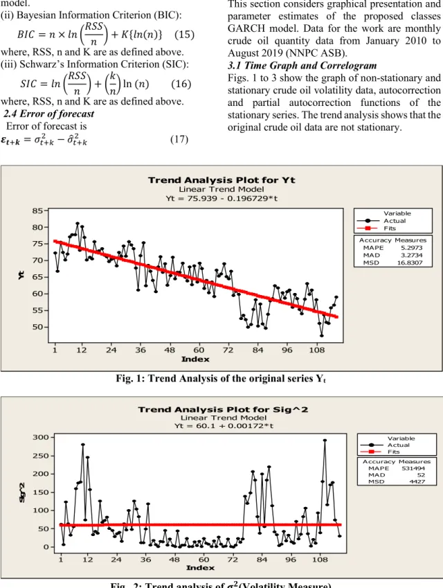
Figs. 1 to 3 show the graph of non-stationary and stationary crude oil volatility data, autocorrection and partial autocorrection functions of the stationary series. The trend analysis shows that the original crude oil data are not stationary.
Fig. 1: Trend Analysis of the original series Yt
Fig. 2: Trend analysis of 𝝈𝒕𝟐(Volatility Measure)
108 96 84 72 60 48 36 24 12 1 85 80 75 70 65 60 55 50 Index Y t MA PE 5.2973 MA D 3.2734 MSD 16.8307 A ccuracy Measures A ctual Fits Variable
Trend Analysis Plot for Yt
Linear Trend Model Yt = 75.939 - 0.196729*t 108 96 84 72 60 48 36 24 12 1 300 250 200 150 100 50 0 Index S ig ^ 2 MA PE 531494 MA D 52 MSD 4427 A ccuracy Measures A ctual F its Variable
Trend Analysis Plot for Sig^2
Linear Trend Model Yt = 60.1 + 0.00172* t
The above graph is the trend analysis of the stationary volatility measure of the crude oil quantity data. There is exhibition of wide swings
at some periods, especially in 2010, 2012, 2016 and 2019, indicating significant variability in the series.
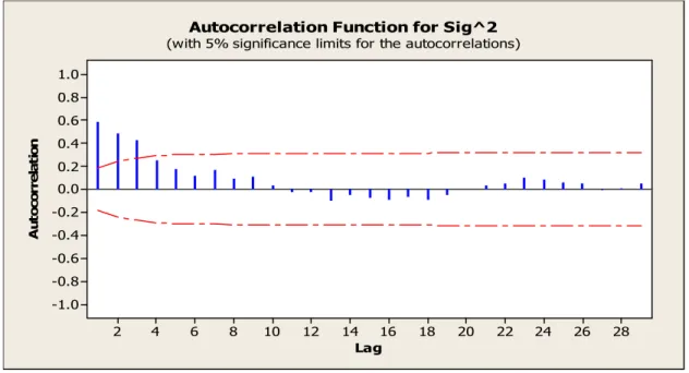
Fig. 3: Autocorrelation Function of the variance, 𝝈𝒕𝟐(Volatility Measure)
Fig. 4: Partial Autocorrelation Function of the variance, 𝝈𝒕𝟐(Volatility Measure) From Fig. 3 and 4, the lag length is 2, determining
the order of the model. Conspicuously, there is exponential decay in the autocorrelation function and significant cut-off at the first 2 lags in the
partial autocorrelation function. Hence, GARCH (0, 1), GARCH (0,2), GARCH (1,1), GARCH (1,2), GARCH (2,1) and GARCH (2,2) are suggested for the crude oil volatility series.
28 26 24 22 20 18 16 14 12 10 8 6 4 2 1.0 0.8 0.6 0.4 0.2 0.0 -0.2 -0.4 -0.6 -0.8 -1.0 Lag A u to co rr e la ti o n
Autocorrelation Function for Sig^2
(with 5% significance limits for the autocorrelations)
28 26 24 22 20 18 16 14 12 10 8 6 4 2 1.0 0.8 0.6 0.4 0.2 0.0 -0.2 -0.4 -0.6 -0.8 -1.0 Lag P a rt ia l A u to co rr e la ti o n
Partial Autocorrelation Function for Sig^2
3.2 Model specification
(i) GARCH (p,q) Model Given the GARCH model
𝜎 = 𝜔 + 𝛼 𝜎 + 𝛽 𝜖 19)
where 𝜎 is the variance measure, 𝛼 and 𝛽 are the parameters of the lagged variance and squared error respectively, 𝜖 ~𝑁(0, 𝜎 ), special orders of p and q are considered for estimation of parameters.
Parameter Estimates different GARCH (p,q) Model
Parameter estimates for the alternative GARCH model are presented below (i.e Table 1)
Table 1: Estimates with regression model using MINITAB
3.3 Model Selection
This section presents the criteria for the selection of the more suitable model for forecast. The information is presented in Table 2.
From Table 2, the two competitive models selected for further comparison using error of forecast are GARCH (1,2) and GARCH (2,1). Table2: Information criteria
S/
N Model Specification AIC BIC SIC
1 GARCH (0,1) 8.2490 951.3904 8.2730 2 GARCH (0,2) 8.1595 935.6597 8.2075 3 GARCH (1,1) 8.0226 928.0937 8.0704 4 GARCH (1,2) 7.9792 917.841 8.0512 5 GARCH (2,1) 7.9875 918.7872 8.0512 6 GARCH (2,2) 7.9881 921.5854 8.0841
3.4 Forecast function and error of forecast
3.4.1: The estimated GARCH (1,2) model is
𝜎 = 22.3 + 0.541𝜎 − 0.00078𝜖 + 0.00281𝜖 (20) 3.4.2: The estimated GARCH (2,1) model is
𝜎 = 19.5 + 0.475𝜎 + 0.225𝜎 − 0.00041𝜖 (21) 3.4.3: Forecast function for GARCH (1,2) is
𝜎 = 22.3 + 0.541𝜎 −
0.00078𝜖 + 0.00281𝜖 (22) 3.4.4: Forecast function for GARCH (2,1) is
𝜎 = 19.5 + 0.475𝜎 + 0.225𝜎 − 0.00041𝜖 (23) 3.4.5: Error of Forecast Error of forecast is 𝜺𝒕 𝒌= 𝜎 − 𝜎 (24) 𝑀𝑆𝐸(𝜺𝒕 𝒌) = 𝐸(𝜎 − 𝜎 )𝟐 (25) 𝑀𝑆𝐸(𝜀 ) of GARCH (1,2) model is 5392 𝑀𝑆𝐸(𝜀 ) of GARCH (2,1) model is 5369. The analysis and estimates of the parameters of the six suggested models are in Table 1. The “t” and “p” values of the coefficients have revealed the parameters that are significant and those that are not. From the results, all the parameters of GARCH (0, 1) and GARCH (2,2) are significant. The contributions of 𝜖 to GARCH (1,1), GARCH (1,2) and GARCH (2,1) and 𝜎 , 𝜖
and 𝜖 to GARCH (2,2) are not significant as evident in the t and p values of the parameter estimates. With the outcome of the parameter estimates of the suggested models, different model selection criteria are used to detect the best of the GARCH models. The Akaike Information Criterion (AIC), Bayesian Information Criterion (BIC) and Schwarz’s Information Criterion (SIC) adopted have revealed two competitive models, and these are GARCH (1,2) and GARCH (2,1). GARCH (1,2) model has 0.0083 and 0.9462 AIC and BIC values less than GARCH(2,1). The AIC and BIC values of the two models places GARCH (1,2) model superior to GARCH (2,1) model in modelling the crude oil production volatility data. Looking at the mean square error of forecast from the two models, GARCH (2,1) has a value 23 mean square error less than GARCH (1,2), placing the model on a higher comparative advantage in forecast than the other. The two models GARCH (1,2) and GARCH (2,1) are comparatively good, but the latter is recommended for better forecast of the Nigerian crude oil production volatility series. Further findings may reveal other alternative models as the crude oil production pattern changes in the future.
4.0 Conclusion
Incontrovertibly, crude oil production quantity has triggered serious concern as much as price, given the fact that the two economic variables constitute a determinant factor to the amount of revenue derived from oil sector in any oil producing nation. In as much as crude oil production quantity has significant effect on the revenue, routine research investigations on the production quantity are advocated. Due to certain political, economic, social, insecurity factors, crude production sometimes dwindles in quantity, therefore, accounts for volatility in the production quantity. This explains the need to develop series of time series models to capture the asymmetry of the crude oil production pattern. The popular GARCH (p,q) model has been explored with different orders of “p” and “q”, producing alternative GARCH models for the crude o107-196il production volatility series. Information criteria adopted have placed GARCH (1,2) and GARCH (2,1) models on comparative advantage. The superiority of GARCH (2,1) over GARCH (1,2) is on the mean square error of forecast. Notwithstanding the findings in this study, further researches about crude oil production quantity volatility and its effect on the nation’s economy are very pertinent.
5.0 References
Babatunde S. Omotosho & Sani I. Doguwa (2012).Under the dynamics of inflation volatility in Nigeria: A GARCH perpective.
CBN Journal of Applied Statistics, 3, 2, 51-71.
Bollerslev, T. (1986). Generalised
autoregressive conditional heteroskedasticity.
Journal of Econometrics, 31, 3, pp.
307-327.
Box, G. P. & Jenkins, G. M. (1976). Time series
analysis, forecasting and control.
Holden-Day, San Francisco.
Claudia, K., Ross, M. & Alexander, S. (2004). A continuous-time GARCH process driven by a levy process: Stationary and second-order behaviour. Journal of Applied Probability, 41, 3, pp. 601-622.
Bala, D. A. & Asemota, J. O. (2013). Exchange rate volatility in Nigeria: Application of GARCH models with exogenous break. CBN
Journal of Applied Statistics, 4,1, pp..89-116.
David, A. L. (2018). Modelling volatility persistence and asymmetry with exogenous breaks in the Nigerian stock returns. CBN
Journal of Applied Statistics, 9, 1, pp.107-196.
Dong, L., Xingfa, Z., Ke, Z. & Shiqing, L. (2018). The ZD-GARCH model; A new way to study heteroskedasticity. Journal of
Econometrics, 202, 1, pp. 1-17.
Engle, R. F. (1982). Autoregress107ive conditional heteroskedasticity with estimates of the variance of United Kindom Inflation.
Econometrica, 50, 4, pp. 987-1007.
Engle, R. F. & Ng, V. K. (1993). Measuring and testing the impact of news on volatility.
Journal of Finance, 48, 5, pp. 1749 – 1778.
Franses, P. H. (1998). Time series models for business and economic forecast. Journal of
Time Series Analysis, 16, pp.509-529.
Glosten, L. R., Jagannathan, R. & Runke, D. E (1993). On the relationship between the expected value and the volatility of the nominal excess return on stocks. Journal of
Finance, 48, pp. 1779-1801.
Gujarati, D. N. & Porter, D. C. (2009). Basic
Econometrics, Fifth Edition.
Hentschel, L. (1995). All in the family Nesting symmetric and asymmetric GARCH models.
Journal of Financial Econometrics, 39, 1, pp.
71-104.
Isenah, M. G., Agwuegbo, S. O. N. & Adewole, A. P. (2013).Analysis of Nigerian Stock Market Returns Using Skewed
ARMA-GARCH Model. Journal of the Nigerian
Statistical Association, 25, pp. 31-50. . .
Ismail O. F. & Oluwasegun, B. A. (2017). Modeliing inflation rate volatility in Nigeria with structural breaks. CBN Journal of Applied
Statistics, 8, 1, pp. 175-193.
Nelson, D. B. (1991). Conditional heteroskedasticity in asset returns: A new approach. Econometrica, 59, pp. 347-370. NNPC Annual Statistical Bulletin (2019).
https://www.nnpcgroup.com/NNPCDocume nts/Annual%20Statistics%20Bulletin%E2%80 %8B/ASB%201918%201st%20Edition.pdf Onyeka-Ubaka J. N., Okafor R. O. & Abass O.
(2018). Trading volume volatility in Nigeria’s banking sector. Benin Journal
of Statistics, 1, pp. 21-32.
Philip I. N. & Omolade , A.(2017). Determinants of FDI and FPI Volatility: An E-GARCH Approach. CBN Journal of Applied Statistics, 8, 2, pp. 47-67
Philipp, O., Wolfgang, S. & Robert, G. (2018). Generalised spartial and spatiotemporal autoregressive conditional heteroskedasticity.
Spartial Statistics, 26, pp. 125-145.
Reuben, O. D., Hussaini, G. D. & Shehu U. G. (2016). Modelling volatility of the exchange rate of the naira to major currencies. CBN
Journal of Applied Statistics,17, 2, pp.
159-187.
Sentana, E. (1995). Quadratic ARCH models.
Review of Econometric Studies, 62, pp.
639-661.
Stephen, O. U., Victor, N. A. & Farida, U. (2015). Nigeria dtock market volatility in comparison with some countries: Application of asymmetric GARCH models. CBN
Journal of Applied Statistics, 6, 2, pp. 133-160.
Storti, G. & Vitale, C. (2003): BL-GARCH models and asymmetries in volatility.
Statistical Methods and Applications, 12, pp.
19-39.
Yaya, O. S. (2013) Nigerian stock index: A search for optimal GARCH model using high frequency data. CBN Journal of Applied
Statistics, 4. 2. Pp. 69-85.
Yaya, O. S. & Shittu, O. I. (2014). Naira exchange rate volatility: smooth transition or linear GARCH specification? Journal of the
Nigerian Statistical Association, 26, pp.78-87.
Yaya, O. S., Abiodun S. B. & Ngozi V. A. (2016) Volatility in the Nigerian stock market: Empirical application of beta-t-GARCH variants. CBN Journal of Applied Statistics, 17, 2p.27-48.
Zakoian, J. M. (1994): Threshold heteroskedastic models. Journal of Economic Dynamics
and Control, 18, pp. 931-955.
Appendix 1: Nigeria monthly crude oil production in millions of barrels
2010 2011 2012 2013 2014 2015 2016 2017 2018 2019 JAN 72.29 77 70.71 75.3 71.05 67.63 66.71 56.95 61.19 51.03 FEB 66.78 70.23 68.38 62.36 64.5 61.68 59.58 50.9 56.03 47.32 MARCH 75.57 70.93 72.4 68.56 66.48 64.04 60.87 49.57 59.75 53.69 APRIL 72.42 70.49 71.28 66.82 66.48 60.39 59.8 53.79 58.56 51.39 MAY 70.15 75.66 74.43 64.01 69.25 63.5 52.63 57.96 55.35 51.12 JUNE 71.92 72.63 71.3 60.56 65.06 59.19 53.49 58.6 54.08 55.86 JULY 77.07 72.94 75.66 68.07 63.82 67.04 52.26 62.46 58.42 56.64 AUG 77.7 73.49 74.65 71.12 68.1 65.39 50.04 61.82 63.05 59.06 SEP 77.81 71.56 73.56 66.52 62.69 65.93 50.86 57.92 59.86 OCT 81.2 71.18 67.78 69.08 68.32 69.08 55.3 60.34 61.2 NOV 73 69.73 61.17 62.65 63.6 65.14 58.28 58.75 54.76 DEC 80.13 70.41 71.45 65.43 69.21 64.44 50.25 60.66 58.2