Sample size, skewness and leverage effects in value at risk and expected shortfall estimation

FACULTAD DE CIENCIAS ECONÓMICAS Y

EMPRESARIALES

Departamento de Fundamentos del Análisis Económico II

TESIS DOCTORAL

Sample size, skewness and leverage effects in value at risk and

expected shortfall estimation

Efectos del tamaño muestral, la asimetría y el apalancamiento en la

estimación del valor en riesgo y de la pérdida esperada

MEMORIA PARA OPTAR AL GRADO DE DOCTOR PRESENTADA POR

Laura García Jorcano

Director

Alfonso Novales Cinca

Madrid, 2018

DEPARTAMENTO DE FUNDAMENTOS DEL AN ´ALISIS ECON ´OMICO II

(ECONOMIA CUANTITATIVA)

Doctorado en Banca y Finanzas Cuantitativas

TESIS DOCTORAL

Sample size, skewness and leverage effects in Value at Risk

and Expected Shortfall estimation

Efectos del tama˜

no muestral, la asimetr´ıa y

el apalancamiento en la estimaci´

on del Valor en Riesgo y

de la P´

erdida Esperada

MEMORIA PARA OPTAR AL GRADO DE DOCTOR REALIZADA Y PRESENTADA POR

Laura Garc´ıa Jorcano

DIRECTOR

Alfonso Novales Cinca

DEPARTMENT OF FOUNDATIONS OF ECONOMIC ANALYSIS II (QUANTITATIVE ECONOMICS)

Program in Banking and Quantitative Finance

DOCTORAL THESIS

Sample size, skewness and leverage effects in Value at Risk

and Expected Shortfall estimation

AUTHOR

Laura Garc´ıa Jorcano

ADVISOR

Alfonso Novales Cinca

List of Figures v

List of Tables xi

Resumen 1

Summary 5

1 Probability-unbiased VaR estimator 9

1.1 Introduction . . . 11

1.2 A review of literature . . . 11

1.3 Quantile or VaR estimator . . . 12

1.4 Parametric and Non-Parametric methods . . . 15

1.5 Normal Distribution . . . 16

1.5.1 Parametric probability-unbiased VaR estimator for a Normal distri-bution. . . 18

1.5.2 A comparison of probability-unbiased VaR and plug-in VaR under Normality . . . 23

1.5.3 Bootstrapping estimation of probability-unbiased VaR . . . 25

1.5.4 Approximate probability-unbiased confidence intervals for VaR un-der Normality . . . 27

1.6 Student-t Distribution . . . 31

1.6.1 Probability-unbiased VaR estimator for a Student-t distribution . . 31

1.6.2 A comparison of probability-unbiased VaR and plug-in VaR under Student-t . . . 38

1.6.3 Approximate probability-unbiased confidence intervals for VaR un-der Studen-t . . . 38

1.7 Mixture of two Normal distributions . . . 40

1.7.1 Casuistry of Mixture of two Normal distribution . . . 40

1.7.2 Probability-unbiased VaR estimator for Mixtures of Normal distri-butions . . . 41

1.7.3 A comparison of probability-unbiased VaR and plug-in VaR under Mixtures of Normal distributions . . . 51

1.7.4 Approximate probability-unbiased confidence intervals for VaR un-der Mixtures of Normal distributions . . . 51

Bibliography 61

Appendices 63

A VaRpu calculated with the bootstrap algorithm proposed by FH for a

Nor-mal distribution . . . 65

B Mixture of two distributions . . . 73

2 Volatility specifications versus probability distributions in VaR estima-tion 79 2.1 Introduction . . . 81

2.2 A review of literature . . . 83

2.3 Models and probability distributions . . . 88

2.4 The data . . . 89

2.5 Parameter estimates . . . 92

2.6 Fitting the data . . . 100

2.6.1 Likelihood ratio tests . . . 101

2.6.2 Fitting standardized innovations . . . 102

2.6.2.1 Fitting the empirical distribution of return innovations . . 102

2.6.2.2 Fitting the sample moments of return innovations . . . 105

2.6.3 Fitting observed returns . . . 111

2.6.3.1 Fitting the empirical distribution of asset returns . . . 111

2.6.3.2 Fitting the sample moments of asset returns . . . 112

2.7 VaR Performance . . . 117

2.7.1 Backtesting VaR . . . 117

2.7.2 VaR Analysis . . . 119

2.7.3 Frequency of violations . . . 120

2.7.4 Switching between models . . . 120

2.7.5 Dominance among VaR models . . . 122

2.7.6 Loss functions . . . 125

2.7.7 Model Confidence Sets . . . 125

2.8 Conclusions . . . 130

Bibliography 133 Appendices 143 A Models and Probability distributions . . . 145

A.1 GARCH volatility model . . . 145

A.2 GJR-GARCH volatility model . . . 145

A.3 APARCH volatility model . . . 145

A.4 FGARCH volatility model . . . 146

A.5 Skewed Student-t distribution . . . 147

A.6 Skewed Generalized Error distribution . . . 149

A.7 JohnsonSU distribution . . . 150

B Tables . . . 157

3 Testing ES estimation models: An extreme value theory approach 167 3.1 Introduction . . . 169

3.2 Review of Literature . . . 171

3.3 Background . . . 174

3.3.1 The Mathematical Properties of Risk Measures . . . 174

3.3.1.1 Coherence and Related Properties . . . 174

3.3.1.2 Elicitability . . . 175

3.3.1.3 Conditional Elicitability . . . 176

3.3.1.4 Robustness . . . 177

3.3.2 Standard Risk Measures . . . 178

3.3.3 Properties of the Standard Risk Measures . . . 178

3.3.4 Estimating risk: Conditional models for the full distribution . . . 181

3.3.5 Estimating risk: Conditional models for extreme events . . . 181

3.3.6 Estimating risk: Filtered Historical Simulation . . . 184

3.4 Data and Estimation Models . . . 186

3.5 Evaluating 1-day ES . . . 189

3.5.1 A Review of Backtesting Approaches . . . 189

3.5.1.1 The Righi & Ceretta Approach . . . 191

3.5.1.2 The Acerbi & Szekely Approaches . . . 193

3.5.1.3 The Graham & P´al Approach . . . 195

3.5.1.4 The Costanzino & Curran and Du & Escanciano Approaches203 3.5.2 Full sample analysis . . . 206

3.5.3 Pre-crisis and crisis periods . . . 220

3.6 Evaluating 10-day ES . . . 235

3.6.1 Scaling law . . . 235

3.6.2 Filtered Historical Simulation . . . 236

3.6.3 10-day historical returns . . . 237

3.7 Conclusions . . . 246

Bibliography 249 Appendices 257 A Elicitability of VaR . . . 259

1.1 Distortion function for the Normal distribution calculated with the para-metric method. The diagonal (black line) represents no distortion. . . 19 1.2 The quantiles of the Normal cdf versus the quantiles of the distorted

Nor-mal cdf calculated with the parametric method. The diagonal (black line) represents no distortion. . . 20 1.3 The true N(0,1) pdf (blue line), the plug-in pdf (red line) and the pdf

of the unbiased cdf (green line). Points on the horizontal axis show the true V aRd_5% (blue point), theplug-in V aRd_5% (red point) and theunbiased

d

V aR5% (green point). . . 22

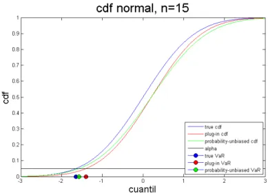
1.4 The true N(0,1) cdf (blue line), the plug-in cdf (red line) and the unbi-ased cdf (green line). Points on the horizontal axis show the true V aRd_5%

(blue point), theplug-inV aRd_5%(red point) and theunbiasedV aRd_5%(green

point) . . . 23 1.5 The true N(0,1) pdf (blue line), the plug-in pdf (red line) and the pdf of

theunbiased cdf (green line) for different sample sizes (enlargement of the left tail). Points on the horizontal axis show the trueV aRd_5% (blue point),

theplug-in V aRd_5% (red point) and the probability-unbiased V aRd_5% (green

point) . . . 24 1.6 The true N(0,1) cdf (blue line), theplug-incdf (red line) and theunbiasedcdf

(green line) for different sample sizes (enlargement of the left tail). Points on the horizontal axis the data points show the true V aRd_5% (blue point),

theplug-inV aRd_5% (red point) and the unbiasedV aRd_5% (green point) . . . 24

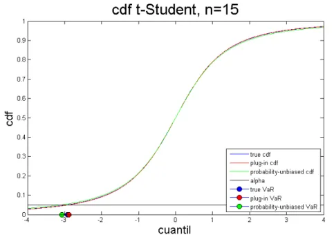
1.7 Distortion function for the Student-t distribution. The diagonal (black line) represents no distorsion. . . 33 1.8 Quantiles of the Student-t cdf versus the quantiles of the distorted Student-t

cdf. The diagonal (black line) represents no distortion. . . 34 1.9 The true t(2) pdf (blue line), the plug-inpdf (red line) and the pdf of the

probabilty-unbiased cdf (green line). On the horizontal axis the data points show the trueV aRd_5% (blue point), the plug-inV aRd _5% (red point) and the

probability-unbiased V aRd_5% (green point) . . . 36

trueV aRd_5%(blue point), theplug-inV aRd_5%(red point) and the

probability-unbiasedV aRd_5% (green point). . . 36

1.11 The true t(2) pdf (blue line), the plug-inpdf (red line) and the pdf of the unbiasedcdf (green line) for different sample sizes (enlargement of the left tail). On the horizontal axis the data points show the true V aRd_5% (blue

point), theplug-inV aRd_5%(red point) and theunbiasedV aRd_5% (green point). 37

1.12 The true t(2) cdf (blue line), the plug-in cdf (red line) and the unbiased cdf (green line) for different sample sizes (enlargement of the left tail). On the horizontal axis the data points show the trueV aRd_5% (blue point), the

plug-inV aRd _5% (red point) and theunbiasedV aRd_5% (green point). . . 37

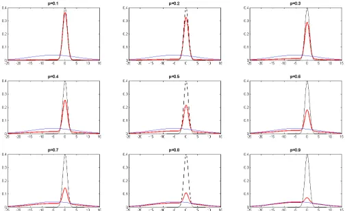
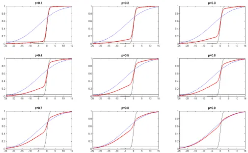
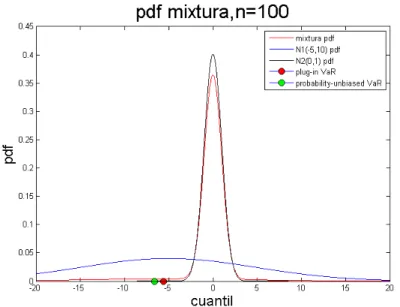
1.13 Density function of the mixture of N1 (-5,10) and N2 (0,1) (red line), density function for N1 (-5,10) (blue line) and density function for N2 (0,1) (black line) for different values of the mixing parameter. . . 41 1.14 Distribution function of the mixture of N1(-5,10) and N2(0,1) (red line),

distribution function for N1(-5,10) (blue line) and distribution function for N2 (0,1) (black line) for different values of the mixing parameter. The black horizontal line indicatesα= 0.05. . . 42 1.15 The mixture density function (red line), the density function of N(0,2) (blue

line) and the density function of N(0,1) (black line). Points on the horizon-tal axis indicate plug-inV aRd_5% (red dot) and probability-unbiased V aRd_5%

(green dot). . . 44 1.16 The mixture distribution function (red line), the distribution function of

N(0,2) (blue line) and the distribution function of N(0,1) (black line). Points on the horizontal axis indicate the points plug-in V aRd_5% (red dot) and

probability-unbiased V aRd_5% (green dot). . . 44

1.17 Mixture density function (red line), density function of N(0,10) (blue line) and density function of N(0,1) (black line). poionts on the horizontal axis indicate plug-in V aRd_5% (red dot) and probability-unbiased V aRd_5% (green

dot). . . 46 1.18 Mixture distribution function (red line), N(0,10) distribution function (blue

line) and N(0,1) distribution function (black line). Points on the horizon-tal axis indicate plug-inV aRd_5% (red dot) and probability-unbiased V aRd_5%

(green dot). . . 46 1.19 Mixture density function (red line), N(-5,2) the density function (blue line)

and N(0,1) density function (black line). Points on the horizontal axis indicate plug-in V aRd_5% (red dot) and probability-unbiased V aRd_5% (green

dot). . . 48 1.20 Mixture distribution function (red line), N(-5,2) distribution function (blue

line) and N(0,1) distribution function (black line). Points on the horizon-tal axis indicate plug-inV aRd_5% (red dot) and probability-unbiased V aRd_5%

(green dot). . . 49 vi

plug-inV aRd _5% (red dot) and probability-unbiasedV aRd_5% (green dot). . . . 50

1.22 Mixture distribution function (red line), N(-5,10) distribution function (blue line) and N(0,1) distribution function (black line). Points on the horizon-tal axis indicate plug-inV aRd_5% (red dot) and probability-unbiased V aRd_5%

(green dot). . . 51 1.23 Portfolio log-returns from 1992 to 2003 and i.i.d. VaR estimates for different

α based on a Student-t rolling window model with a window length of 20 observations. . . 58 1.24 Portfolio log-returns from 1992 to 2003 and i.i.d. VaR estimates for different

α based on a Student-t rolling window model with window length of 200 observations. . . 58 25 Distorsion function for the Normal distribution using bootstrapping

pro-posed by FH. The diagonal (black line) represents no distorsion. . . 66 26 The quantiles of the Normal cdf versus the quantiles of the distorted

Nor-mal cdf using bootstrapping proposed by FH. The diagonal (black line) represents no distortion. . . 66 27 The true N(0,1) pdf (blue line), theplug-inpdf (red line) and the pdf of the

probabilty-unbiased cdf (green line). Points on the horizontal axis show the trueV aRd_5%(blue point), theplug-inV aRd_5%(red point) and the

probability-unbiased V aRd_5% (green point) . Here we use bootstrapping proposed by

FH to calculateαpu. . . 69

28 The true N(0,1) cdf (blue line), theplug-incdf (red line) and the probability-unbiasedcdf (green line). Points on the horizontal axis show the trueV aRd_5%

(blue point), the plug-in V aRd_5% (red point) and the probability-unbiased d

V aR5% (green point) . Here we use bootstrapping proposed by FH to

calculateαpu. . . 69

29 The true N(0,1) pdf (blue line), theplug-inpdf (red line) and the pdf of the probability-unbiased cdf (green line) for different sample sizes (enlargement of the left tail). Points on the horizontal axis show the true V aRd_5% (blue

point), theplug-in V aRd_5% (red point) and the probability-unbiased V aRd_5%

(green point). Here we use the bootstrapping algorithm proposed by FH to calculateαpu . . . 70

30 The true N(0,1) pdf (blue line), theplug-inpdf (red line) and the probability-unbiasedcdf (green line) for different sample sizes (enlargement of the left tail). Points on the horizontal axis show the true V aRd_5% (blue point),

theplug-in V aRd_5% (red point) and the probability-unbiased V aRd_5% (green

point) . Here we use the bootstrapping algorithm proposed by FH to cal-culateαpu . . . 70

31 Density function of the mixture of N1(0,2) and N2(0,1) (red line), the den-sity function N1(0,2) (blue line) and denden-sity function N2(0,1) (black line) for different values of the mixing parameter. . . 74

(black line) for different values of the mixing parameter. The black hori-zontal line indicates theα= 0.05. . . 75 33 Density function of the mixture of N1(0,10) and N2(0,1) (red line), the

density function N1(0,10) (blue line) and density function N2(0,1) (black line) for different values of the mixing parameter. . . 75 34 Distribution function of the mixture of N1(0.10) and N2(0.1) (red line),

the distribution function N1(0.10) (blue line) and the distribution function N2(0, 1) (black line) for different values of the mixing parameter. The black horizontal line indicates theα= 0.05. . . 76 35 Density function of the mixture of N1(-5,2) and N2(0,1) (red line), the

density function N1(-5,2) (blue line) and density function N2(0,1) (black line) for different values of the mixing parameter. . . 77 36 Distribution function of the mixture of N1(-5,2) and N2(0,1) (red line),

the distribution function N1(-5,2) (blue line) and the distribution function N2(0,1) (black line) for different values of the mixing parameter. The black horizontal line indicates theα= 0.05. . . 78 2.1 Stock market indices daily percentage returns and QQ-plot against the

Nor-mal distribution. . . 91 2.2 Histograms and QQ-plots of standardized innovations from SKST-APARCH

model for stock market indices against the skewed Student-t distribution. . 99 2.3 News impact curves of different volatility model for IBM. . . 100 2.4 ζ-histograms (100 cells) for 4173 one-step-ahead forecasts. We assume

dif-ferent distributions with AR(1)-FGARCH(1,1) model for difdif-ferent assets. . 104 5 Region for Skewness-Kurtosis for which Skewed Student-t and JohnsonSU

distributions exist. . . 152 3.1 Profile likelihood for ξ in threshold excess model of percentage daily loss

filtered residuals of IBM with JSU-EVT model. . . 189 3.2 Empirical distribution of excess of IBM filtered residuals of

AR(1)-APARCH(1,1)-JSU and its fitted GPD. . . 190 3.3 The smooth curve through the points shows the estimated tail of the IBM

percentage loss filtered residuals of AR(1)-APARCH(1,1)-JSU using tail estimator. Points are plotted at empirical tail probabilities calculated from empirical distribution function. . . 190 3.4 IBM daily percentage returns and V aR1% and V aR5% calculated with all

sample as well as using only extreme values. . . 208 3.5 IBM daily percentage returns andES1%andES5%calculated with all

sam-ple as well as using only extreme values. . . 209 3.6 Evolution of the ESα/V aRα ratio calculated with EVT from model

JSU-APARCH for IBM. . . 209 3.7 Cumulative hits (violations) of IBM with model APARCH and

JSU-EVT-APARCH for different α. . . 217 viii

3.9 Sample autocorrelations of cumulative hits (violations) of IBM under model JSU-APARCH and JSU-EVT-APARCH for different values of α. . . 218 3.10 Sample autocorrelations of cumulative hits (violations) of SAN under model

JSU-APARCH and JSU-EVT-APARCH for different values of α. . . 219 3.11 Tail-distributions for IBM. N is the Normal distribution, ST is the

Student-t(4.67), SKST is the Skewed Student-t(0.97, 4.69), SGED is the Skewed Generalized Error(0.99, 1.15) and JSU is the Johnson SU (-0.092, 1.53) distribution. . . 219

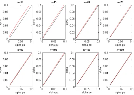
1.1 Probabilitiesαpu(%) to be used to obtain theprobability-unbiasedV aRαfor

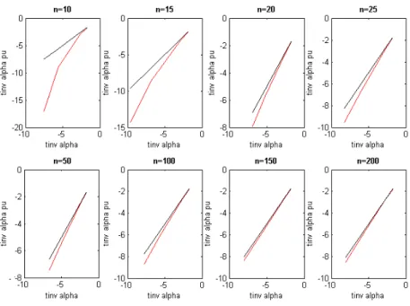
different values of α andn in the i.i.d. Normal distribution case. . . 18 1.2 The shortfall probabilities α(%) with which the next observation is lower

than the plug-in VaR estimatezαpu for the Normal distribution case. . . 19

1.3 Probability-unbiasedV aRd_α versusplug-in V aRd_α in the case of Normal(0,1). 21

1.4 Estimated standard deviations for the distorted distribution function. . . . 22 1.5 Shortfall probabilitiesα% that the next observation will be lower than the

plug-inV aRd and theprobability unbiasedV aRd in the Monte-Carlo

simula-tion for the Normal distribusimula-tion. . . 25 1.6 Probabilities αpu to be used to obtain a probability-unbiased V aRα for

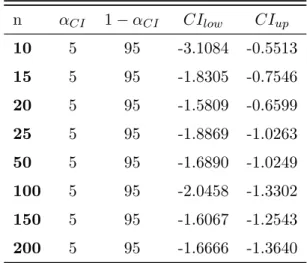
dif-ferent values of α and nin the i.i.d. Normal distribution case using boot-strapping proposed by FH. . . 27 1.7 Probability αCI(%), 1−αCI(%) and quantiles corresponding to the lower

and upper bounds of confidence interval 90% for a Normal distribution. . . 30 1.8 Probabilities αCI,pu(%) such that αCI =P(CI < V aRc ) withα

d

V aR=α =

5% in theV aRd and quantiles corresponding to the lower and upper bounds

of confidence interval 90% in the case of the Normal distribution. . . 30 1.9 Probabilities αpu(%) to be used to obtain a probability-unbiased V aRα for

different values of α andn in the i.i.d. Student-t distribution case. . . 32 1.10 Probability-unbiased V aRd_α versus plug-in V aRd_α in the case of Student-t

distribution. . . 33 1.11 Shortfall probabilities α(%) for the next observation being lower than the

plug-in VaR estimatet−1(αpu). . . 34

1.12 Degrees of freedom estimated for the distorted distribution function. . . 35 1.13 Shortfall probabilities α% that the next observation is always lower than

theplug-inV aRd and the probabilityprobability-unbiasedV aRd in the

Monte-Carlo simulation for Student-t distribution. . . 38 1.14 Probability αCI(%), 1−αCI(%) and quantiles corresponding to the lower

and upper bounds of a 90% plug-in confidence interval in the case of the Student-t distribution. . . 39 1.15 Probabilities αCI,pu(%), αCI = P(CI < V aRc ), with α

d

V aR = α = 5%.

Columns 4 and 5 show the quantiles corresponding to the lower and upper bounds of the 90% confidence interval in the case of the Student-t distribution. 39

1.17 Probabilitiesαpu(%) needed to obtain probability-unbiasedV aRd_α for

sam-ples of size 100, 200, 300 y 400 of a mixture distribution of a Normal(0,2) and of a Normal(0,1) with mixing parameterp= 0.1 and respective probability-unbiasedVaR andplug-in VaR forα= 1% and α= 5%. . . 43 1.18 First four moments for samples of size 100, 200, 300 and 400 of a mixture

distribution of N(0,10) and N(0,1) with mixing parameterp= 0.1. . . 45 1.19 Probabilities αpu(%) needed to obtain the probability-unbiased V aRd_α for

samples of size 100, 200, 300 y 400 of a mixture distribution of a Nor-mal(0,10) and of a Normal(0,1) with mixing parameter p= 0.1. The table also presents the associatedprobability-unbiasedVaR andplug-inVaR esti-mates forα= 1% and α= 5%. . . 45 1.20 First four moments for samples of size 100, 200, 300 and 400 of a mixture

distribution of N(-5,2) and N(0,1) with a mixing parameterp= 0.1. . . 47 1.21 Probabilities αpu(%) needed to obtain probabily-unbiased V aRd_α for

sam-ples of size 100, 200, 300 y 400 of a mixture distribution of a Normal(-5,2) and of a Normal(0,1) with mixing parameter p = 0.1 . We also show the associatedprobability-unbiasedVaR andplug-inVaR forα = 1% andα= 5%. 48 1.22 First four moments for samples of size 100, 200, 300 and 400 of a mixture

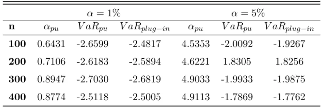
distribution of N(-5,10) and N(0,1) with a mixing parameterp= 0.1. . . 49 1.23 Probabilitiesαpu(%) needed to obtain probability-unbiasedV aRd_α for

sam-ples of size 100, 200, 300 y 400 of a mixture distribution of a Normal(-5,10) and of a Normal(0,1) with mixing parameter p = 0.1 . We also show the associatedprobability-unbiasedVaR andplug-inVaR forα = 1% andα= 5%. 50 1.24 Shortfall probabilitiesα% that the next observation is lower than theplug-in

[

V aR or lower that the probabilityprobability-unbiased V aR[ in the Monte-Carlo simulation, for different mixture distributions. . . 52 1.25 Probability αCI(%), 1−αCI(%) and quantiles corresponding to the lower

and upper bounds of confidence interval 90% for different mixture distribu-tions. . . 52 1.26 Probabilities αCI,pu(%) such that αCI =P([CI < V aR) withα_{V aR[} =α =

5% in theV aR[ and quantiles corresponding to the lower and upper bounds of confidence interval 90% for the different cases of the mixture distribution. 53 1.27 Number of 5% VaR exceedences per year for the i.i.d. mixture rolling

window model with window length n. Absolute differences between the expected number of exceedences (13 per year) and the number of observed exceedences are reported in parentheses. . . 55 1.28 Historical 1% VaR exceedence probabilities of the various models and

his-torical Observed Absolute Deviation (OAD) per year. . . 56 1.29 Historical 5% VaR exceedence probabilities of the various models and

his-torical Observed Absolute Deviation (OAD) per year. . . 57 30 Probability-unbiasedV aRd_α versus plug-inV aRd_α in the case of Normal

dis-tribution (0,1) using bootstrapping proposed by FH. . . 65 xii

calculateαpu. . . 67

32 Estimated standard deviations for the distorted distribution function using bootstrapping proposed by FH to calculateαpu. . . 68

33 Shortfall probabilitiesα% that the next observation will be lower than the plug-in V aRd and the probability probability-unbiased V aRd in the Monte-Carlo simulation for Normal distribution using bootstrapping proposed by FH. . . 71

2.1 Overview of papers that compare VaR models. . . 87

2.2 Overview of papers that compare VaR models (continued). . . 88

2.3 Descriptive statistics for the daily percentage returns. . . 90

2.4 Parameter estimates of APARCH model for stock market indices under different probability distributions. . . 94

2.5 Parameter estimates of the APARCH model for individual stocks under different probability distributions. . . 95

2.6 Parameter estimates of the APARCH model for interest rates under differ-ent probability distributions. . . 96

2.7 Parameter estimates of the APARCH model for commodities under different probability distributions. . . 97

2.8 Parameter estimates of the APARCH model for exchange rates under dif-ferent probability distributions. . . 98

2.9 Likelihood ratio tests of volatility specifications for stock market indices. Note: The null hypothesis is rejected, except where indicated by boldface. . 101

2.10 Goodness-of-fit tests for standardized innovations of stock market indices. Figures in brackets denote p-value. . . 102

2.11 Absolute differences between standardized innovation moments and theo-retical moments for stock market indices. . . 106

2.12 Absolute differences between standardized innovation moments and theo-retical moments for individual stocks. . . 107

2.13 Absolute differences between standardized innovation moments and theo-retical moments for interest rates. . . 108

2.14 Absolute differences between standardized innovation moments and theo-retical moments for commodities. . . 109

2.15 Absolute differences between standardized innovation moments and theo-retical moments for exchange rates. . . 110

2.16 Goodness-of-fit tests for observed returns of stock market indices. Figures denote the fail rates for each model. . . 112

2.17 Empirical moments vs sample moments for stock market indices. . . 114

2.18 Empirical moments vs sample moments for individual stocks. . . 115

2.19 Empirical moments vs sample moments for interest rates. . . 115

2.20 Empirical moments vs sample moments for commodities. . . 116

2.21 Empirical moments vs sample moments for exchange rates. . . 116 xiii

model for all assets. . . 122 2.23 Dominance among VaR models. C1 is the set consisting of the number

of times H0 is rejected with D1/M1 for the different assets, C2 is the set consisting of the number of times H0 is rejected with D2/M2 for the different assets andpis the proportion of times that H0 is rejected with D2/M2 and and also rejected with D1/M1. . . 124 2.24 Composition of remaining probability distribution-volatility model

combi-nations in the Superior Set for each asset discriminated by model and dis-tribution according QLF loss function (top panel) and AlTick loss function (bottom panel). . . 129 2.2 V aR_1% results with GARCH volatility model for all assets: unconditional

coverage test, independence and conditional coverage tests and Dynamic Quantile Test. P-values are reported in parentheses. For each model, the first line shows the number of VaR excesses produced with the different assets (boldface). . . 157 2.3 V aR1% results with GJRGARCH volatility model for all assets:

uncondi-tional coverage test, independence and condiuncondi-tional coverage tests and Dy-namic Quantile Test. P-values are reported in parentheses. For each model, the first line shows the number of VaR excesses produced with the different assets (boldface). . . 158 2.4 V aR1% results with APARCH volatility model for all assets: unconditional

coverage test, independence and conditional coverage tests and Dynamic Quantile Test. P-values are reported in parentheses. For each model, the first line shows the number of VaR excesses produced with the different assets (boldface). . . 159 2.5 V aR_1% results with FGARCH volatility model for all assets: unconditional

coverage test, independence and conditional coverage tests and Dynamic Quantile Test. P-values are reported in parentheses. For each model, the first line shows the number of VaR excesses produced with the different assets (boldface). . . 160 2.6 V aR1% loss functions for stock market indices: Quadratic Loss Function

(QLF) and Asymmetric Linear Tick Loss Function (AlTick). . . 161 2.7 V aR1%loss functions for individual stocks: Quadratic Loss Function (QLF)

and Asymmetric Linear Tick Loss Function (AlTick). . . 162 2.8 V aR_1% loss functions for interest rates: Quadratic Loss Function (QLF)

and Asymmetric Linear Tick Loss Function (AlTick). . . 163 2.9 V aR_1%loss functions for commodities: Quadratic Loss Function (QLF) and

Asymmetric Linear Tick Loss Function (AlTick). . . 164 2.10 V aR1% loss functions for exchange rates: Quadratic Loss Function (QLF)

and Asymmetric Linear Tick Loss Function (AlTick). . . 165 3.1 Properties of standard risk measures (Emmeret al., 2015 [39]) . . . 181 3.2 Descriptive statistics for the daily percentage returns. . . 186

correspond to the standard error of shape parameter and scale parameter. . 188 3.4 Parameter estimates of AR(1)-APARCH(1,1) model with JSU distribution

for IBM and with GPD for IBM residuals of the previous model. . . 188 3.5 Overview of ES backtesting procedures in literature. . . 191 3.6 Descriptive statistics for the log-returns (%) of four indexes for in-sample

and out-of-sample period. JB stat is the statistic of Jarque-Bera test. . . . 207 3.7 Descriptive Analysis of Violations for IBM and SAN with

AR(1)-APARCH(1,1)-JSU and with AR(1)-APARCH(1,1)-EVT-AR(1)-APARCH(1,1)-JSU. . . 212 3.8 Mean estimates, violations ratio and backtesting results (p-values) for ES

estimates from all the models for IBM.BTT is the test of Righi & Ceretta, Z1 and Z2 are the tests of Acerbi & Szekely, T R is the test of Graham &

P´al, andUES,CES(1) andCES(5) are the unconditional and the conditional

(lags= 1 andlags= 5) tests of Costanzino & Curran and Du & Escanciano. The p-values in bold indicate that the statistics obtained in these tests have an opposite sign to that specified in the alternative hypothesis. . . 213 3.9 Mean estimates, violations ratio and backtesting results (p-values) for ES

estimates from all the models for SAN.BTT is the test of Righi & Ceretta, Z1 and Z2 are the tests of Acerbi & Szekely, T R is the test of Graham &

P´al, andUES,CES(1) andCES(5) are the unconditional and the conditional

(lags = 1 and lags = 5) tests of Costanzino & Curran and Du & Escan-ciano.The p-values in bold indicate that the statistics obtained in these tests have an opposite sign to that specified in the alternative hypothesis. . . 214 3.10 Mean estimates, violations ratio and backtesting results (p-values) for ES

estimates from all the models for AXA.BTT is the test of Righi & Ceretta, Z1 and Z2 are the tests of Acerbi & Szekely, T R is the test of Graham &

P´al, andUES,CES(1) andCES(5) are the unconditional and the conditional

(lags= 1 andlags= 5) tests of Costanzino & Curran and Du & Escanciano. The p-values in bold indicate that the statistics obtained in these tests have an opposite sign to that specified in the alternative hypothesis. . . 215 3.11 Mean estimates, violations ratio and backtesting results (p-values) for ES

estimates from all the models for BP.BTT is the test of Righi & Ceretta,Z1

andZ2 are the tests of Acerbi & Szekely, T Ris the test of Graham & P´al,

and UES, CES(1) and CES(5) are the unconditional and the conditional

(lags = 1 and lags = 5) tests of Costanzino & Curran and Du & Escan-ciano.The p-values in bold indicate that the statistics obtained in these tests have an opposite sign to that specified in the alternative hypothesis. . . 216 3.12 Mean estimates, violations ratio and backtesting results (p-values) for ES

estimates from all the models for IBM and for 1-day returns calculated by FHS. BTT is the test of Righi & Ceretta and Z1 and Z2 are the tests of

Acerbi & Szekely. The p-values in bold indicate that the statistics obtained in these tests have an opposite sign to that specified in the alternative hypothesis. . . 221

FHS. BTT is the test of Righi & Ceretta and Z1 and Z2 are the tests of

Acerbi & Szekely. The p-values in bold indicate that the statistics obtained in these tests have an opposite sign to that specified in the alternative hypothesis. . . 222 3.14 Mean estimates, violations ratio and backtesting results (p-values) for ES

estimates from all the models for AXA and for 1-day returns calculated by FHS. BTT is the test of Righi & Ceretta and Z1 and Z2 are the tests of

Acerbi & Szekely. The p-values in bold indicate that the statistics obtained in these tests have an opposite sign to that specified in the alternative hypothesis. . . 223 3.15 Mean estimates, violations ratio and backtesting results (p-values) for ES

estimates from all the models for BP and for 1-day returns calculated by FHS. BTT is the test of Righi & Ceretta and Z1 and Z2 are the tests of

Acerbi & Szekely. The p-values in bold indicate that the statistics obtained in these tests have an opposite sign to that specified in the alternative hypothesis. . . 224 3.16 Sample information about the different considered periods. . . 225 3.17 Mean estimates, violations ratio and backtesting results (p-values) for ES

estimates from all the models for IBM and for pre-crisis period. BTT is the

test of Righi & Ceretta, Z1 and Z2 are the tests of Acerbi & Szekely, T R

is the test of Graham & P´al, and UES,CES(1) and CES(5) are the

uncon-ditional and the conuncon-ditional (lags = 1 and lags = 5) tests of Costanzino & Curran and Du & Escanciano. The p-values in bold indicate that the statistics obtained in these tests have an opposite sign to that specified in the alternative hypothesis. . . 227 3.18 Mean estimates, violations ratio and backtesting results (p-values) for ES

estimates from all the models for SAN and for pre-crisis period. BTT is the

test of Righi & Ceretta, Z1 and Z2 are the tests of Acerbi & Szekely, T R

is the test of Graham & P´al, and UES,CES(1) and CES(5) are the

uncon-ditional and the conuncon-ditional (lags = 1 and lags = 5) tests of Costanzino & Curran and Du & Escanciano. The p-values in bold indicate that the statistics obtained in these tests have an opposite sign to that specified in the alternative hypothesis. . . 228 3.19 Mean estimates, violations ratio and backtesting results (p-values) for ES

estimates from all the models for AXA and for pre-crisis period. BTT is

the test of Righi & Ceretta, Z1 and Z2 are the tests of Acerbi & Szekely,

T Ris the test of Graham & P´al, andUES,CES(1) andCES(5) are the

un-conditional and the un-conditional (lags= 1 andlags= 5) tests of Costanzino & Curran and Du & Escanciano. The p-values in bold indicate that the statistics obtained in these tests have an opposite sign to that specified in the alternative hypothesis. . . 229

test of Righi & Ceretta, Z1 and Z2 are the tests of Acerbi & Szekely, T R

is the test of Graham & P´al, and UES,CES(1) and CES(5) are the

uncon-ditional and the conuncon-ditional (lags = 1 and lags = 5) tests of Costanzino & Curran and Du & Escanciano. The p-values in bold indicate that the statistics obtained in these tests have an opposite sign to that specified in the alternative hypothesis. . . 230 3.21 Mean estimates, violations ratio and backtesting results (p-values) for ES

estimates from all the models for IBM and for crisis period. BTT is the

test of Righi & Ceretta, Z1 and Z2 are the tests of Acerbi & Szekely, T R

is the test of Graham & P´al, and UES,CES(1) and CES(5) are the

uncon-ditional and the conuncon-ditional (lags = 1 and lags = 5) tests of Costanzino & Curran and Du & Escanciano. The p-values in bold indicate that the statistics obtained in these tests have an opposite sign to that specified in the alternative hypothesis. . . 231 3.22 Mean estimates, violations ratio and backtesting results (p-values) for ES

estimates from all the models for SAN and for crisis period. BTT is the

test of Righi & Ceretta, Z1 and Z2 are the tests of Acerbi & Szekely, T R

is the test of Graham & P´al, and UES,CES(1) and CES(5) are the

uncon-ditional and the conuncon-ditional (lags = 1 and lags = 5) tests of Costanzino & Curran and Du & Escanciano. The p-values in bold indicate that the statistics obtained in these tests have an opposite sign to that specified in the alternative hypothesis. . . 232 3.23 Mean estimates, violations ratio and backtesting results (p-values) for ES

estimates from all the models for AXA and for crisis period. BTT is the

test of Righi & Ceretta, Z1 and Z2 are the tests of Acerbi & Szekely, T R

is the test of Graham & P´al, and UES,CES(1) and CES(5) are the

uncon-ditional and the conuncon-ditional (lags = 1 and lags = 5) tests of Costanzino & Curran and Du & Escanciano. The p-values in bold indicate that the statistics obtained in these tests have an opposite sign to that specified in the alternative hypothesis. . . 233 3.24 Mean estimates, violations ratio and backtesting results (p-values) for ES

estimates from all the models for BP and for crisis period. BTT is the test of

Righi & Ceretta,Z1andZ2 are the tests of Acerbi & Szekely,T Ris the test

of Graham & P´al, andUES,CES(1) and CES(5) are the unconditional and

the conditional (lags= 1 andlags= 5) tests of Costanzino & Curran and Du & Escanciano. The p-values in bold indicate that the statistics obtained in these tests have an opposite sign to that specified in the alternative hypothesis. . . 234

FHS. BTT is the test of Righi & Ceretta and Z1 and Z2 are the tests of

Acerbi & Szekely. The p-values in bold indicate that the statistics obtained in these tests have an opposite sign to that specified in the alternative hypothesis. . . 238 3.26 Mean estimates, violations ratio and backtesting results (p-values) for ES

estimates from all the models for SAN and for 10-day returns calculated by FHS. BTT is the test of Righi & Ceretta and Z1 and Z2 are the tests of

Acerbi & Szekely. The p-values in bold indicate that the statistics obtained in these tests have an opposite sign to that specified in the alternative hypothesis. . . 239 3.27 Mean estimates, violations ratio and backtesting results (p-values) for ES

estimates from all the models for AXA and for 10-day returns calculated by FHS.BTT is the test of Righi & Ceretta and Z1 and Z2 are the tests of

Acerbi & Szekely. The p-values in bold indicate that the statistics obtained in these tests have an opposite sign to that specified in the alternative hypothesis. . . 240 3.28 Mean estimates, violations ratio and backtesting results (p-values) for ES

estimates from all the models for BP and for 10-day returns calculated by FHS. BTT is the test of Righi & Ceretta and Z1 and Z2 are the tests of

Acerbi & Szekely. The p-values in bold indicate that the statistics obtained in these tests have an opposite sign to that specified in the alternative hypothesis. . . 241 3.29 Mean estimates, violations ratio and backtesting results (p-values) for ES

estimates from all the models for IBM and for 10-day returns calculated as the sum of 10 daily logarithmic returns not overlapped. BTT is the test of

Righi & Ceretta,Z1andZ2 are the tests of Acerbi & Szekely,T Ris the test

of Graham & P´al, andUES,CES(1) and CES(5) are the unconditional and

the conditional (lags= 1 andlags= 5) tests of Costanzino & Curran and Du & Escanciano. The p-values in bold indicate that the statistics obtained in these tests have an opposite sign to that specified in the alternative hypothesis. . . 242 3.30 Mean estimates, violations ratio and backtesting results (p-values) for ES

estimates from all the models for SAN and for 10-day returns calculated as the sum of 10 daily logarithmic returns not overlapped. BTT is the test of

Righi & Ceretta, Z1 and Z2 are the tests of Acerbi & Szekely, T R is the

test of Graham & P´al, andUES,CES(1) and CES(5) are the unconditional

and the conditional (lags= 1 andlags= 5) tests of Costanzino & Curran and Du & Escanciano. The hyphen means that there are no violations. The p-values in bold indicate that the statistics obtained in these tests have an opposite sign to that specified in the alternative hypothesis. . . 243

as the sum of 10 daily logarithmic returns not overlapped. BTT is the test

of Righi & Ceretta,Z1 and Z2 are the tests of Acerbi & Szekely, T R is the

test of Graham & P´al, andUES,CES(1) and CES(5) are the unconditional

and the conditional (lags= 1 andlags= 5) tests of Costanzino & Curran and Du & Escanciano. The hyphen means that there are no violations. The p-values in bold indicate that the statistics obtained in these tests have an opposite sign to that specified in the alternative hypothesis. . . 244 3.32 Mean estimates, violations ratio and backtesting results (p-values) for ES

estimates from all the models for BP and for 10-day returns calculated as the sum of 10 daily logarithmic returns not overlapped. BTT is the test of

Righi & Ceretta, Z1 and Z2 are the tests of Acerbi & Szekely, T R is the

test of Graham & P´al, andUES,CES(1) and CES(5) are the unconditional

and the conditional (lags= 1 andlags= 5) tests of Costanzino & Curran and Du & Escanciano. The hyphen means that there are no violations. The p-values in bold indicate that the statistics obtained in these tests have an opposite sign to that specified in the alternative hypothesis. . . 245

La estimaci´on de las medidas de riesgo es un ´area de gran importancia en la industria financiera. Las medidas de riesgo juegan un papel principal en la gesti´on del riesgo y en el c´alculo del capital requerido. El documento Basilea III [13] ha sugerido medir el riesgo en condiciones de tensi´on mediante la P´erdida Esperada (ES), en lugar del Valor en Riesgo (VaR), a un nivel de confianza del 97.5%. Este cambio viene motivado por las atractivas propiedades te´oricas del ES como medida de riesgo y por las limitaciones del VaR. En particular, el VaR no captura el ”riesgo de cola”. En esta transici´on, el principal reto al que se enfrentan las instituciones financieras es la falta de disponibilidad de herramientas sencillas para la evaluaci´on de las predicciones del ES, esto es,backtestingdel ES.

El objetivo de la tesis es comparar laperformancede una variedad de modelos para la estimaci´on del VaR y del ES para un conjunto de activos de diferente naturaleza: ´ındices de mercado, acciones, bonos, tipos de cambio y materias primas. A lo largo de la tesis, entendemos por “modelo” VaR o por “modelo” ES una especificaci´on dada por un modelo de volatilidad condicional combinado con una distribuci´on de probabilidad que suponemos siguen las innovaciones estandarizadas.

En concreto, el Cap´ıtulo 1 considera el concepto de insesgadez en la estimaci´on del VaR. Francioni y Herzog (2012) [FH] [20] demuestran que existe una correcci´on anal´ıtica del sesgo del VaR cuando los rendimientos siguen una distribuci´on Normal. En este cap´ıtulo, el an´alisis FH se extiende a la distribuci´on t-Student as´ı como a la Mixtura de dos Nor-males, utilizando el algoritmo bootstrapping propuesto por FH. El uso de medidas VaR insesgadas en probabilidad evita la infraestimaci´on sistem´atica del riesgo como resultado del sesgo que presentan las medidas VaR est´andar. La magnitud de la distorsi´on necesaria para pasar del cuantil del VaR est´andar al del VaR insesgado en probabilidad depende del tama˜no de la muestra y del supuesto de distribuci´on de los rendimientos. Debido a que la distribuci´on de los rendimientos financieros tiene colas m´as gruesas que la Normal, a menor tama˜no muestral y menor grosor de las colas de la distribuci´on supuesta en la estimaci´on, mayor es la distorsi´on necesaria para obtener un estimador insesgado. Este ajuste del VaR nos permite trabajar con muestras peque˜nas con la tranquilidad de que se obtendr´a una buenaperformance del VaR. Adem´as, los resultados obtenidos en la tesis demuestran que las muestras peque˜nas permiten obtener estimaciones del VaR m´as exac-tas que las muestras grandes seg´un la Probabilidad en Exceso y la Desviaci´on Absoluta Observada por a˜no (media de las diferencias absolutas entre el n´umero esperado de exce-sos y el n´umero observado de excesos respecto del VaR). La buenaperformance del VaR

financieras debido al comportamiento del mercado.

El Cap´ıtulo 2 analiza como la eficiencia del VaR depende de la especificaci´on de volatil-idad y del supuesto acerca de la distribuci´on de probabilidad para las innovaciones de las rentabilidades. Esta cuesti´on es crucial para los gestores de riesgo debido a la existencia de un gran n´umero de posibles elecciones de modelos de volatilidad y de distribuciones de probabilidad, siendo conveniente establecer algunas prioridades al modelar los rendimien-tos para estimar el riesgo. Consideramos diferentes modelos VaR condicionales para ac-tivos de diferente naturaleza, utilizando distribuciones sim´etricas y asim´etricas para las innovaciones y modelos de volatilidad con y sin efecto apalancamiento. El VaR estimado se calcula siguiendo el enfoque param´etrico. La capacidad para explicar los momentos muestrales de las rentabilidades podr´ıa considerarse una condici´on natural para obtener una buenaperformance del VaR. Sin embargo, aunque hay normalmente un esfuerzo sig-nificativo para seleccionar una combinaci´on apropiada de distribuci´on de probabilidad y especificaci´on de volatilidad en la estimaci´on del VaR, la capacidad para explicar los momentos muestrales de las rentabilidades rara vez se examina. Tras la utilizaci´on de m´etodos de simulaci´on para calcular los momentos de las rentabilidades impl´ıcitos a par-tir de los modelos estimados, comparamos los niveles impl´ıcitos de asimetr´ıa y curtosis de las rentabilidades con sus momentos muestrales an´alogos. Se observa que la capacidad para explicar los momentos muestrales est´a, de hecho, ligada a la performance del VaR. Dicha performance es examinada a trav´es de contrastes est´andar: el contraste de cober-tura incondicional de Kupiec (1995) [78], el de cobercober-tura condicional y de independencia de Christoffersen (1998) [27] y el Dynamic Quantile de Engle y Manganelli (2004) [39], as´ı como, a trav´es de funciones de p´erdida propuestas por Lopez (1998, 1999) [85] [86] y Sarma et al. (2003) [113] y por Giacomini y Komunjer (2005) [47].

Respecto a una literatura cada vez m´as abundante, contribuimos de diferentes formas: i) considerando un conjunto de distribuciones de probabilidad que recientemente han sido consideradas apropiadas para capturar la asimetr´ıa y la curtosis de datos financieros, pero cuyaperformancepara las estimaciones del VaR no ha sido comparada previamente para una base de datos com´un: distribuci´on t-Student asim´etrica [41], Error Generalizada asim´etrica [41], Johnson SU [70], t-Generalizada asim´etrica [123] y t-Student asim´etrica

Hiperb´olica Generalizada [1], junto con las distribuciones Normal y t-Student como bench-mark,

ii) considerando tres especificaciones de volatilidad con apalancamiento, GJR-GARCH, APARCH y FGARCH, as´ı como el modelo est´andar sim´etrico GARCH comobenchmark. Los modelos FGARCH y APARCH son cada vez m´as apreciados al ser adecuados para las rentabilidades financieras ya que su especificaci´on considera una potencia en la desviaci´on est´andar de las innovaciones lo que proporciona mayor flexibilidad a la din´amica de la volatilidad,

iii) evaluando expl´ıcitamente el ajuste de las rentabilidades y relacionando esa capaci-dad de ajuste con laperformance del VaR e

iv) introduciendo un criterio de dominancia para establecer un ranking de modelos en

Obtenemos los siguientes resultados:

i) los modelos VaR que asumen distribuciones de probabilidad asim´etrica para las in-novaciones, como la t-Student asim´etrica, la Error Generalizada asim´etrica, la JohnsonSU

y la t-Generalizada asim´etrica proporcionan un mejor ajuste de los momentos muestrales de las rentabilidades que las distribuciones sim´etricas y logran una mejorperformancedel VaR,

ii) los modelos de volatilidad con apalancamiento, como el APARCH y el FGARCH, muestran una mejor performance del VaR que las especificaciones de volatilidad m´as est´andar como el GARCH y el GJR-GARCH,

iii) los resultados de nuestras simulaciones fuera de muestra sugieren que el supuesto importante para la performance del VaR es el de la distribuci´on de probabilidad de las innovaciones de las rentabilidades, jugando un papel secundario la elecci´on del modelo de volatilidad,

iv) la consideraci´on de la potencia de la desviaci´on est´andar condicional como un par´ametro libre es una importante caracter´ıstica de las especificaciones de volatilidad APARCH/FGARCH, al sugerir nuestras estimaciones, para un n´umero considerable de activos, que la especificaci´on de la desviaci´on condicional al cuadrado es inapropiada,

v) un buen ajuste de los momentos de las rentabilidades normalmente conlleva una buenaperformancedel VaR. Los modelos APARCH o FGARCH con distribuciones Error Generalizada asim´etrica, t-Generalizada asim´etrica y JohnsonSU son preferidos a aquellos

con otras distribuciones asim´etricas, como la t-Student asim´etrica y la t-Student asim´etrica Hiperb´olica Generalizada, o con distribuciones sim´etricas, como la t-Student y la Normal y

vi) modelos VaR alternativos parecen proporcionar distinta performance del VaR para las diferentes clases de activos.

En el Cap´ıtulo 3 estimamos el ES condicional basado en el enfoque de la Teor´ıa de Valores Extremos (EVT) utilizando distribuciones de probabilidad asim´etricas para las in-novaciones de las rentabilidades y examinamos la exactitud de nuestras estimaciones antes y durante la crisis financiera de 2008 utilizando datos diarios a horizontes 1 d´ıa y 10 d´ıas. Tenemos en cuenta los efectos de los agrupamientos de volatilidad y de apalancamiento en la volatilidad de las rentabilidades al utilizar un modelo APARCH con diferentes dis-tribuciones de probabilidad para las innovaciones estandarizadas: Gaussiana, Student, t-Student asim´etrica, Error Generalizada asim´etrica y JohnsonSU, as´ı como, con el enfoque

EVT siguiendo el procedimiento de dos pasos de McNeil y Frey (2000) [75]. Este pro-cedimiento en dos pasos ajusta la distribuci´on Pareto Generalizada a los valores extremos de los residuos estandarizados generados por los modelos APARCH. Posteriormente, com-paramos la performance de las predicciones del ES fuera de muestra un d´ıa hacia adelante de todos estos modelos para diferentes niveles de significaci´on (α). Previamente, los con-trastes de backtesting existentes para ES han demostrado tener serias limitaciones, como son el contraste de McNeil y Frey (2000) [75], de Berkowitz (2001) [15], de Kerkhof y Me-lenberg (2004) [65] y de Wong (2008) [95]. Tales limitaciones son superadas por algunas

(2014) [4], que son sencillos pero requieren an´alisis de simulaci´on (como el contraste de Righi y Ceretta), el contraste de Graham y P´al (2014) [57], que es una extensi´on del enfoque Lugannani-Rice de Wong, el contraste de cobertura incondicional de Costanzino y Curran (2015) [26] para la familia de medidas de riesgo espectrales, de la cual el ES es miembro y, finalmente, el contraste condicional de Du y Escanciano (2015) [36].

Este cap´ıtulo contribuye a la literatura de diferentes maneras:

i) considerando la especificaci´on de volatilidad APARCH en modelos EVT utilizando Simulaci´on Hist´orica Filtrada (FHS), lo que permite considerar los agrupamientos de volatilidad y la asimetr´ıa de los rendimientos,

ii) comparando modelos EVT condicionales que incorporan modelos condicionales con distribuciones de probabilidad asim´etricas apenas utilizadas en la literatura financiera para la estimaci´on del ES,

iii) analizando la performance de las estimaciones del VaR y del ES a horizonte 10 d´ıas, tal y como proponen los requerimientos de capital de Basilea,

iv) centr´andonos en la exactitud de nuestros modelos de riesgo para estimar el VaR y el ES durante los periodos de pre-crisis y de crisis, as´ı como, para diferentes niveles de significaci´on (α) y

v) evaluando la performance del ES con las propuestas m´as recientes de backtesting para ES, considerando todas en el mismo estudio.

Obtenemos las siguientes conclusiones:

i) la Teor´ıa de Valores Extremos produce una buena estimaci´on del ES independiente-mente de la distribuci´on de probabilidad supuesta en la estimaci´on para las innovaciones de las rentabilidades. Esto es debido al hecho de que la cola, para todos estos casos, es modelizada con una distribuci´on Pareto Generalizada,

ii) si consideramos modelos condicionales sin el enfoque EVT, observamos que la dis-tribuci´on Error Generalizada asim´etrica y la Johnson SU juegan un papel importante en

la captura del ”riesgo de cola” a horizontes 1 y 10 d´ıas. Esto se debe a que los hechos estilizados de las rentabilidades financieras tales como agrupamientos de volatilidad, colas pesadas y asimetr´ıa son capturados adecuadamente por las mismas,

iii) incluso durante el periodo de crisis, los modelos EVT condicionales son m´as ade-cuados y fiables para predecir las p´erdidas generadas por riesgo de los activos que los modelos condicionales que no incorporan el enfoque EVT y

iv) los modelos EVT condicionales producen, en algunos casos, sobreestimaci´on del ES.

The estimation of risk measures is an area of highest importance in the financial industry. Risk measures play a major role in the risk-management and in the computation of regula-tory capital. The Basel III document [13] has suggested to shift from Value-at-Risk (VaR) into Expected Shortfall (ES) as a risk measure and to consider stressed scenarios at a new confidence level of 97.5%. This change is motivated by the appealing theoretical proper-ties of ES as a measure of risk and the poor properproper-ties of VaR. In particular, VaR fails to control for “tail risk”. In this transition, the major challenge faced by financial institu-tions is the unavailability of simple tools for evaluation of ES forecasts (i.e. backtesting ES) The objective of this thesis is to compare the performance of a variety of models for VaR and ES estimation for a collection of assets of different nature: stock indexes, individual stocks, bonds, exchange rates, and commodities. Throughout the thesis, by a VaR or an ES “model” is meant a given specification for conditional volatility, combined with an assumption on the probability distribution of return innovations.

Specifically, Chapter 1 considers the concept of unbiasedness in VaR estimation. Fran-coni and Herzog (2012) (FH) [20] showed that there exists an analytical bias correction for VaR when returns are Normally distributed. In this chapter the FH analysis is extended to the Student-t distribution as well as to Mixtures of two Normal distributions, using a bootstrapping algorithm proposed by FH. The use of the probability-unbiased VaR avoids the systematic underestimation of risk implied by the bias of standard VaR measures. The magnitude of the distortion that needs to be exerted on the quantile to move from the standard VaR to the probability-unbiased VaR depends on the sample size and on the distribution assumption on returns. Since financial returns usually have thick tails, the smaller the sample size and the lower the heaviness of the tail of the assumed distribution in estimation, the higher will be the distortion to be applied to achieve unbiasedness. This VaR adjustment allows us to work with small samples knowing that the estimated VaR will generally display a good performance. Furthermore, the results in the thesis show that using a small sample may easily lead to more accurate VaR estimates than longer samples according to the Exceedance Probability and to the Observed Absolute Deviation per year (mean of the absolute differences between the expected number of exceedances and the number of observed exceedances). The good performance of the probability-unbiased VaR follows from the fact that a short sample size allows for capturing better the structural changes that arise over time in financial returns due to trading behaviour.

is crucial for risk managers, since there are so many potential choices for volatility model and probability distributions that it would be very convenient to establish some priorities in modelling returns for risk estimation. We consider different conditional VaR models for assets of different nature, using symmetric and asymmetric probability distributions for the innovations and volatility models with and without leverage. We calculate VaR esti-mates following the parametric approach. The ability to explain sample return moments might be considered a natural condition to obtain a good VaR performance. However, even though significant effort is usually placed in selecting an appropriate combination of probability distribution and volatility specification in VaR estimation, the ability to explain sample return moments is seldom examined. After using simulation methods to calculate implied return moments from estimated models, we compare the implied levels of skewness and kurtosis of returns with the analogue sample moments. We show that the ability to explain sample moments is in fact linked to performance in VaR estimation. Such performance is examined through standard tests: the unconditional coverage test of Kupiec (1995) [78], the independence and conditional coverage tests of Christoffersen (1998) [27], the Dynamic Quantile test of Engle and Manganelli (2004) [39], as well as the loss functions proposed by Lopez (1998, 1999) [85] [86] and Sarma et al. (2003) [113] and that of Giacomini and Komunjer (2005) [47].

Relative to an ever increasing literature, we contribute in different ways:

i) considering a set of probability distributions that have recently been rendered to be appropriate for capturing the skewness and kurtosis of financial data, but whose perfor-mance for VaR estimation has not been compared previously on a common dataset: Skewed Student-t [41], Skewed Generalized Error [41], JohnsonSU [70], Skewed Generalized-t [123]

and Generalized Hyperbolic Skew Student-t [1] distributions, with the Normal and sym-metric Student-t distributions as benchmark,

ii) considering three volatility specifications with leverage, GJR-GARCH, APARCH and FGARCH, as well as the standard symmetric GARCH model as benchmark. FGARCH and APARCH are increasingly being appreciated as being adequate for financial returns because they are specified for a power of the conditional standard deviation of the inno-vations, which provides more flexibility to the dynamics of volatility,

iii) explicitly evaluating the fit to return data, relating that fitting ability to VaR performance, and

iv) by introducing a dominance criterion to establish a ranking of models on the basis of their behavior under standard VaR validation tests and loss functions.

We obtain the following results:

i) VaR models that assume asymmetric probability distributions for the innovations, like the Skewed Student-t distribution, Skewed Generalized Error distribution, Johnson SU distribution, and Skewed Generalized-t distribution provide a better fit to sample re-turn moments than symmetric distributions and achieve a better VaR performance,

ii) volatility models with leverage, like APARCH and FGARCH, show a better VaR performance than more standard GARCH and GJR-GARCH volatility specifications,

choice of volatility model playing a secondary role,

iv) dealing with the power of the conditional standard deviation as a free parameter is an important feature of the APARCH/FGARCH volatility specifications because our estimates suggest that for a number of financial assets the squared conditional deviation specification is inappropriate,

v) a good fit to return moments usually leads to a good VaR performance. APARCH or FGARCH models with Skewed Generalized Error, Skewed Generalized-t and Johnson SU distributions are preferred to other asymmetric distributions, like Skewed Student-t

and Generalized Hyperbolic Skew Student-t, and symmetric distributions, like Student-t and Normal distributions, and

vi) alternative VaR models seem to provide a distinct performance for different classes of assets.

In Chapter 3 we estimate the conditional Expected Shortfall based on the Extreme Value Theory (EVT) approach using asymmetric probability distributions for return inno-vations, and we analyze the accuracy of our estimates before and during the 2008 financial crisis using daily data for 1- and 10-day horizons. We take into account volatility cluster-ing and leverage effects in return volatility by uscluster-ing the APARCH model under different probability distributions assumed for the standardized innovations: Gaussian, Student-t, skewed Student-t, skewed generalized error and Johnson SU and under EVT methods,

following the two-step procedure of McNeil & Frey (2000) [75]. This two-step procedure fits a Generalized Pareto Distribution to the extreme values of the standardized residuals generated by APARCH models. Then, we compare the one-step-ahead out-of-sample ES forecast performance of all these models for different significance levels (α). Previously existing backtesting tests for ES have been shown have serious limitations [as McNeil & Frey (2000) [75] test, Berkowitz (2001) [15] test, Kerkhof and Melenberg (2004) [65] test and Wong (2008) [95] test]. Such limitations are overcome by some recent ES backtesting proposals that we use for ES evaluation: the Righi & Ceretta (2013) [83] test, two tests by Acerbi & Szekely (2014) [4] that are straightforward but require simulation analysis (like the Rigui & Ceretta test), the test of Graham & P´al (2014) [57], which is an extension of the Lugannani-Rice approach of Wong, the quantile-space unconditional coverage test of Costanzino & Curran (2015) [26] for the family of Spectral Risk Measures, of which ES is a member and, finally, the conditional test of Du & Escanciano (2015) [36].

This chapter contributes to the literature in different ways:

i) considering the APARCH volatility specification in an EVT model using Filtered Historical Simulation (FHS) [11] [12] to take into account volatility clustering and asym-metric returns,

ii) comparing conditional EVT models that incorporate conditional models with asym-metric probability distributions rarely used in the financial literature for ES estimation,

iii) by analyzing the performance of VaR and ES estimates over 10-day horizons for risk liquidity management, as proposed in Basel capital requirements [13],

iv) by focusing on the accuracy of our risk models for VaR and ES estimation during

the same study.

We obtain the following conclusions:

i) Extreme Value Theory produces a good ES performance regardless of the probabil-ity distribution assumed for return innovations in estimation. This is due to the fact that the tail is modeled with a Generalized Pareto Distribution not only with 1-day but also 10-day horizons,

ii) if we consider conditional models without the EVT approach, we observe that the Skewed Generalized Error distribution and the JohnsonSU distribution play an important

role in capturing tail risk in 1-day and 10-day horizons. This is because the stylized facts of financial returns such as volatility clusters, heavy tails and asymmetry are suitably captured by these asymmetric distributions,

iii) even during the crisis period, conditional EVT models are more accurate and re-liable for predicting asset risk losses than conditional models that do not incorporate the EVT approach, and

iv) sometimes conditional EVT models produce a ES overestimation.

Probability-unbiased VaR

estimator

Abstract

The Probability unbiasedness of a Value at Risk (VaR) estimator guarantees that the numerical VaR estimate obtained from a finite amount of data will be exceeded by the next observation drawn from the same distribution with an expected probabilityα. In the special case of a Normal distribution, closed-formed solutions for probability unbiased VaR estimators are known. For the general case, we use a bootstrapping algorithm to illustrate the outcomes obtained by estimating VaR from simulated random samples of different length generated from Normal, Student-t and Mixtures of two Normal distributions. Using the empirical distribution derived for the VaR estimate, we compute in short samples the probability-unbiased VaR as well as its confidence bands. Our results show that short samples may yield good VaR estimates. In fact, we show the probability unbiased VaR estimator to display a better performance than the standard VaR estimator obtained under different models, all of which are much more complex.

The parametric or variance-covariance approach to the estimation of VaR in two steps: first, the distribution is estimated by statistical methods; in the second step, the estimated distribution is considered as the true distribution and VaR is computed. In the parametric case this is achieved by using the mathematical expression for VaR in each specific model and inserting the estimated parameters. This VaR estimator is calledplug-in estimator. It is well-known that the highly nonlinear mapping from the model parameters to the risk-measure introduces biases and some statistical experiments show that this bias leads to a systematic underestimation of risk.

VaR performance is usually assessed by comparing the observed number of violations of the quantile estimator threshold with the theoretical frequency. Francioni and Herzog, “Probability-unbiased Value-at-Risk estimators” [20] suggest the use of probability unbi-asedness as a criterion to judge the quality of VaR estimates. Probability unbiunbi-asedness means that the VaR estimator should be unbiased regarding the relative frequency of vio-lations of the quantile. They show how theα-quantile may be modified so that the implied VaR estimate is unbiased.

We use the non-parametric method (bootstrapping) for the calculation of the unbi-ased VaR estimator introduced by Francioni and Herzog for the Normal distribution. We extend their approach to other distributions such as Student-t and mixture of Normals, while using the parametric approach to calculate probability-unbiased VaR in the Normal case. We show that the use of probability-unbiased VaR avoids the systematic underes-timation of risk implied by the bias of standard VaR measures in small samples. The magnitude of the distortion that needs to be exerted on the quantile to move from the standard VaR to the probability-unbiased VaR depends on the sample size and on the distribution assumption on returns. Our results suggest that using a small sample may easily lead to more accurate VaR estimates than a historical estimator based on long sam-ples according to the exceedence probability and to the Observed Absolute Deviation per year. Short samples are more robust to the structural changes that may arise over time in financial returns due to trading behavior.

The remainder of the chapter is organized as follows. In Section 1.2, we present a review of literature. In Section 1.3, we describe the concept of quantile or VaR estima-tor. In Section 1.4, we introduce the difference between parametric and non-parametric methods used to calculate probability-unbiased VaR. In Sections 1.5, 1.6 and 1.7, we ex-plain and calculate probability-unbiased VaR with Normal, Student-t and Mixture of two Normal distributions, respectively. In Section 1.8, we report the results of an empirical application. Finally, Section 1.9 concludes the chapter.

1.2

A review of literature

The estimation of risk measures is an area of highest importance in the financial industry. Risk measures play a major role in the risk-management and in the computation of

latory capital. [For an in-depth treatment of the topic, see textbooks of McNeil, Frey and Embrechts (2005) [75] and of Alexander (2009) [2]]. In particular, Embrechts and Hofert (2014) [37] highlight that a major part of quantitative risk management is actually of sta-tistical nature, and the stasta-tistical aspects in the estimation of risk measures have recently raised a lot of attention [see Acerbi and Szekely (2007) [4], Davis (2014) [10], Emmer et al. (2015) [39], Du and Escanciano (2015) [36], Costanzino and Curran (2015) [26], Fissler et al. (2015) [45] and Ziegel (2016) [97]]. Surprisingly, it turns out that statistical properties of risk estimators have not yet been analyzed thoroughly. Some of the existing analysis show that standard risk estimators may be biased, and they systematically underestimate risk. Unfortunately, while the classical (statistical) definition of bias is always desirable from a theoretical point of view, it is not considered a priority by financial institutions or regulators, for whom the backtests are the main source of estimation accuracy.

Not surprisingly, the occurrence of biases in risk estimation plays an important role in practice. The Basel III document [13] has suggested to shift from Value-at-Risk into Expected Shortfall as a risk measure and to consider stressed scenarios at a new confi-dence level of 97.5%. In fact, such a correction may reduce the bias, but only in the right scenarios. Our goal is to obtain probability-unbiased estimators that pass the standard backtesting procedure proposed by Basel. That amounts to having an expected failure rate close to the theoretical VaR levelα.

Francioni and Herzog (2012) [20] (FH) have shown how to distort the α quantile used in VaR estimation so that the implied VaR estimator is unbiased in probability, in a sense to be defined below. Our goal is to extend the concept of probability unbiased estimation introduced by FH to distributions different from Normal. In this line, Pitera and Schmidt (2016) [26] propose an unbiased bootstrapping estimator under Normality obtained by distorting the estimated parameters of the distribution instead of distorting the VaR confidence level as FH suggest. The FH strategy is the one we follow in this chapter.

1.3

Quantile or VaR estimator

In this section we describe the concepts associated to the probability unbiased estimation of Value at Risk.

Let us suppose thatX is an absolutely continuous random variable with distribution functionFθ, where θis a parameter vector. The α quantileQα ofX is defined as

Qα =F_θ−1(α)

By definition, the quantile has the property that Fθ(Qα) =α

This equation represents the intuitive concept of the quantile as a threshold that is exceeded with probability α. The quantile Qα of the distribution of returns of a given