DYNAMIC MODEL BASED PREDICTIVE CONTROL FOR MOBILE ROBOTS

DYNAMIC MODEL BASED PREDICTIVE

CONTROL FOR MOBILE ROBOTS

Andrés Rosales, Miguel Peña, Gustavo Scaglia, Vicente Mut, Fernando di Sciascio

Instituto de Automática (INAUT). Universidad Nacional de San Juan

Av. Libertador San Martín 1109 (oeste). J5400ARL. San Juan, Argentina e-mail:{arosales,gscaglia,vmut,fernando,slawinski}@inaut.unsj.edu.ar

Abstract– A nonlinear predictive controller (NMPC) is developed to control a unicycle-like mobile robot for trajectory tracking. Dynamic model of PIONNER 3-DX mobile robot is used, where external forces and wheels sliding have been considered. Restrictions on control actions and system states are also considered. Simulations results at both tracking and regulation (positioning) are shown, these results show the good performance of developed controller. Finally, this paper shows that the controller can be implemented in real-time by using an analysis of compute times of NMPC algorithm.

Key words– mobile robot, predictive nonlinear control (NMPC), trajectory tracking, dynamic model

I. INTRODUCTION

The trajectory tracking control for mobile robots is a fundamental problem, which has been investigated exhaustively by the scientific community. Several papers deal about the design of control laws for mobile robot with its dynamic model, for instance in trajectory tracking (De la Cruz et al., 2006; Dong et al., 2005; Albagul et al., 2004; Yang et al., 1999; Zhang et al., 1998). One of first investigation results for this problem was deal in Kanayama et al. (1990), where author uses the Lyapunov theory to design the tracking controller. Nevertheless, this and others controllers do not take in count the restrictions in the control signals because it is a hard task to implement.

Nonlinear predictive control (NMPC) is a most frequently control-optimization technique used in industry. This methodology has been designed to deal with optimization problems with restrictions. NMPC is an optimization algorithm online to predict output system based on current states and model system, and also, to find a control feature in open loop by using numeric optimization and to apply the first control signal of this optimized feature to system.

In model based predictive control due to use the receding horizon, the stability analysis is one of the main problems (Peña, 2002). Previous works have demonstrated that a finite receding horizon can guarantee NMPC stability even for nonlinear systems

(Camacho et al., 1998; Peña, 2002), although this strategy is considered heavy due to its computational effort in practice. The NMPC stability analysis with finite receding horizon has been studied in Mayne et al. (2000) and Fontes (2001). Recently, the qualities of predictive control have been explored and applied in robotics, woks like Dongbing et al. (2006), Hedjar et al. (2005), Künhe et al. (2005) and Ramírez et al. (1999) show different approaches and strategies in MPC with good results for tracking control and regulation. This paper applies NMPC to dynamic model of mobile robot and makes an analysis by computes times for optimization algorithm so that to be able to implement the controller in experimental works.

The paper is organized as follows: Section II describes the NMPC algorithm and the programming schemes used. Section III shows the dynamic model of mobile robot. Section IV describes the simulation results. Conclusions and future works are detailed in last Section.

II. PREDICTIVE NONLINEAR CONTROL

A general deterministic nonlinear model at discrete time for a system can be expressed like,

(k+ =1)

(

( ) ( )k , k

)

x f x v (1)

( )k =

(

( )k

)

y h x (2)

where, x(k), v(k) and y(k) are the state vector, signal

control and output system respectively.

The most of MPC methods are based on common

scheme (Ramírez et al., 1999). A cost functional J is

defined, which is often a quadratic function with the sum of the norms of future trajectory tracking errors,

(k i k+ | )= (k i k+ | )− d(k i+ )

e y y (3)

predicted over a prediction horizon N plus the sum of the

norms of predicted increments in the control action, over a control horizon Nu,

(

)

2

(

)

2 1 1 1 u N N i i i i J δ k i k λ k i k = = =

∑

+ +

∑

Δ + − Q R e v (4)

(

k i k

) (

k i k

) (

k i 1k

)

Δv + =v + −v + −

where, δi and λi are penalty sequences usually chosen as

constants, yd(k+i) is the desired output and the notation

y(k+i|k) means that y(k+i) is computed with known

information at instant k. Future system outputs y(k+i|k)

for i = 1, …, N, are predicted by using a process model

since the previous outputs and inputs at instant k, and

since the future predicted control actions v(k+i|k) for i =

0, …, Nu-1, which are pretended to compute. Also,

2 ₌ T

Q

x x Qx and Q>0 (Peña, 2002).

On this way J can be expressed like a function that

only depends on future control actions. The predictive control objective is to obtain a sequence of future control actions [v(k), v(k+1|k), …, v(k+Nu-1|k)], so that

predicted outputs y(k+i|k), using the system model, are

so near of reference yd(k+i|k) as it is possible, along the

prediction horizon. This is obtained by means of

minimization of J respect to control variables. After

obtaining this sequence, a receding horizon strategy is

used, which entails applying only the first control action

v(k) computed. This process is repeated every sampling

time.

When nonlinear models are used, MPC depends to find a solution for a nonlinear programming problem in every sampling step. To solve that problem is necessary doing the optimization and solving the system model. Both problems can be implemented by two different ways: sequential or simultaneously (Peña, 2002).

A. Sequential optimization algorithm

In the sequential implementation, a solution at every iteration for the optimization routine is found. Controls are the decision variables, which goes into algorithm and this computes the model solution. Then, this solution is used to evaluate the objective function and the compute value is given to the optimization program. The optimization variable is,

( )k

(

k 1k

)

(

k Nu 1k

)

T

⎡ ⎤

=_⎣ + + − _⎦

z v v L v (5)

First, functional must solve the system model with

vector z values and with current state x(k) applied N

times the Eq. (1). On this way, the vector sequence

(

k 1k

) (

k 2k

)

(

k N k

)

⎡ + + + ⎤

⎣x x L x ⎦ is got, whereas

with Eq. (2) the output values sequence

(

k 1k

) (

k 2k

)

(

k N k

)

⎡ + + + ⎤

⎣y y L y ⎦ is obtained. Then,

the cost functional (Eq. (4)) is evaluated with this values.

The cost functional J depends on predicted outputs,

which are based on state vector as well and this vector is function of control actions (optimization variables). Therefore, results to obtain the functional gradient,

outputs have to derive respect control actions from k to

(k+Nu-1). This is complicated and not always has

solution. Therefore, the sequential resolution has not gradient information and it must be obtained by using numeric differentiation, which is computationally

negative, because this generates greatest calculus cost and convergence problems.

B. Simultaneous optimization algorithm

Unlike sequential solution, simultaneous solution and optimization includes states and controls of model like decision variables. Model equations are added to the optimization problem like restriction equations. Then, the optimization variable results,

( )

(

)

(

)

( )

(

)

(

)

1 1 1 _u 1 T k k k k N k k k k k N k ⎡ =_⎣ + + + ⎤ + + − _⎦ z x x x v v v L L (6)

in other words, the states and control actions are considered like optimization variables. The dimension of

this vector is (eN + pNu), which is bigger than sequential

approach dimension (pNu), where e and p are sizes of

state vector and control input, respectively. This entails a considerable increase in the optimization variable size in relation to sequential approach.

Model equations appear like equality restrictions as follows in Eq. (6),

(

)

(

( ) ( )

)

(

)

(

( ) ( )

)

(

)

(

( ) ( )

)

1 , 2 1 , 1 1 , u k k k k k k k k k N k k N k N ⎧ + = ⎪ ⎪ + = + + = ⎨ ⎪ ⎪ _{+ = + − +} ⎩ x f x v x f x v R x f x v M (6)

In this approach, the gradient obtaining by analytic way is simplest, so that, the optimization algorithm is able to incorporate in an explicit way. By using the functional in Eq. (4) results Eq. (7). The equality restrictions gradient is a disperse matrix (Eq. (8)).

(

)

(

)

( )

(

)

(

)

( )

(

)

(

)

( ) ( ) ( ) ( ) ( ) ( ) 1 2 1 2 1 2 2 3 2 1 1 2 2 2 2 2 2 1 2 1 2 2 2 1 k k k N u T d T d T N d N u k k k k k k k N k k N J k k k k k N δ δ δ λ λ λ λ λ + + + ⎡ ⎡_⎣ + − + ⎤_⎦ ⎤ ⎢ ⎥ ⎢ _{⎡ + − + ⎤} ⎥ ⎢ ⎣ ⎦ ⎥ ⎢ ⎥ ⎢ ⎥ ⎢ _{⎡ + − + ⎤}⎥ ∇ =_{⎢ ⎣ ⎦⎥} ⎢ _{Δ − Δ +} ⎥ ⎢ ⎥ Δ + − Δ + ⎢ ⎥ ⎢ ⎥ ⎢ ⎥ ⎢ Δ + − ⎥ ⎣ ⎦ x x x G Q h x y G Q h x y G Q h x y R v R v R v R v R v M M (7) ( ) ( )

(

)

( ) , i T k i k k k = ∂ = ∂ x h x v G x ( ) ( ) ( ) ( ) ( ) 1 0 0 0 0 0 0 0 1 0 0 0 0 0 0 0 1 0 0 0 0 0 1 e e e e e e e e e e e e e e e e e e e e e e e e e e e e e e e e e e e e e e e e e e e e e e u k k N k k k N × × × × × × × × × × × × × × × × × × × × × × × ⎡ − + ⎤ ⎢ ⎥ ⎢ ⎥ ⎢ ⎥ ⎢ _{− + −} ⎥ ⎢ ⎥ ⎢ ⎥ ∇ =_{⎢ ⎥} − ⎢ ⎥ ⎢ _{− +} ⎥ ⎢ ⎥ ⎢ ⎥ ⎢ _{− + −} ⎥ ⎣ ⎦ I Fx I I Fx R I Fv Fv Fv L L M M O M M L L L L M M O M M L (8)

where,

(

( ) ( )

)

( ) , k i k i k k k + = ∂ = ∂ x f x v F x ,

(

( ) ( )

)

( ) , k i k i k k k + = ∂ = ∂ v f x v F v ,

Iexe is the identity matrix with e dimension and 0pxeis a

null matrix with pxe dimension.

In small problems with few states and short prediction horizon, sequential approach is probably more effective (Peña, 2002). Generally, in big problems simultaneous approach is more robust, because it is less probable that it fails. In sequential approach the addition of restrictions in states or outputs is more complicated. In addition to model restrictions, control actions restrictions, steady state restrictions, etc, can be added.

III. DYNAMIC MODEL OF MOBILE ROBOT

To be able to use MPC strategy is necessary having a mobile robot model. This model will be used to predict future position and orientation of controlled system.

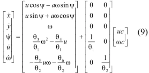
A unicycle-like mobile robot experimentally validated by using PIONNER 3-DX robots in De la Cruz et al. (2006) will be used. A brief model is showed in Fig. 1 and is presented in Eq. (9). The model with more details can be seen on De la Cruz et al. (2006).

The robot position is defined by _h=[ , ]_{x y}T_{, this point is}

located a distance a from rear axle center of the robot, u

and ū are the longitudinal and side speeds of mass

center, ω is the angular speed and ψ is the orientation

angle of the robot, G is the gravity center, B is the base

line center of the wheels, E is the work tool placing

point and C is the castor wheel placing point.

Figure 1: Mobile robot unicycle-like model and its parameters

From model in Fig. 1, the dynamic model of mobile robot is obtaining (De la Cruz et al., 2006),

2 3 4 1 1 1 5 6 2 2 2 cos sin 0 0 sin cos 0 0 0 0 1 0 1 0 u a x u a y uc u c u u ψ − ω ψ ⎡ ⎤ ⎡ ⎤ ⎢ ⎥ ⎢ ⎥ ⎡ ⎤ _⎢ ψ + ω ψ_{⎥ ⎢ ⎥} ⎢ ⎥ ⎢ ω ⎥ ⎢ ⎥ ⎢ ⎥ _{⎢ ⎥ ⎢ ⎥⎡ ⎤} ⎢ ⎥ =ψ ⎢ θ _{ω −}θ ⎥ ⎢+ ⎥⎢ ⎥_ω ⎢ ⎥ _{⎢ θ θ ⎥ ⎢θ ⎥}⎣ ⎦ ⎢ ⎥ ⎢ ⎥ ⎢ ⎥ ⎢ ⎥_{ω ⎢ θ θ ⎥ ⎢ ⎥} ⎣ ⎦ _{− ω − ω} ⎢ _{θ θ} ⎥ ⎢ _θ ⎥ ⎣ ⎦ ⎣ ⎦ & & & & &

(9)

where, the mobile robot parameters, validates in De la Cruz et al. (2006) are,

1 2 3 4 5 6 0.24089 0.2424 0.00093603 0.99629 0.0037256 1.0915 θ = θ = θ = − θ = θ = − θ =

Equation (9) can be wrote in a compact way as follows,

( )

t =

(

( )

t

)

+

(

( )

t

)

x& f x g v (10)

where, x

( )

t =

[

x y ψ u ω

]

T is the state vector of

system and v

_{( )}

t =

[

u_c ω_c

]

T is the control one.

Dynamic model of mobile robot can be discretized by using any numeric approximation approach, for example Euler, in other words,

( ) ( ) 1

k+ = k+To⎡⎣ k + k ⎤⎦

x x f x g v (11)

where, To is the sampling time and the vector of initial

conditions is 0( ) [ 0 0 ψ0 0 ω0]

T

t = x y u

x

.

Equation (12) is the output system,

( )k =

(

( )k

)

= ( )k

y h x Cx (12)

where, C is a matrix oe dimension (o is the state vector

size). In this paper the output equation is given by,

( )k = ⎡_⎣x k( ) y k( ) ψ( )k ⎤_⎦T

y (13)

IV. SIMULATION AND RESULTS

The maximal absolute values of linear and angular speeds of mobile robot used in simulations are 0.5[m/s] and 0.745[rad/s], respectively.

A sampling time To = 0.1[s] was used for all

trajectories and the prediction horizon used was N = Nu

= 7. Furthermore, matrix Q = diag[1, 1, 0.05], matrix R

= I and parameters δ = 28 and λ = 0.8. Linear reference

speed was 0,25[m/s] for both reference trajectories. Reference used values for state ψ, were computed by using Eq. (14), d=atan d d y x ψ ⎛⎜ ⎞⎟ ⎝ ⎠ & & (14) ψ u ω G h a ū E C B y x

First reference trajectory applied to the system was an eight-shaped curve defined by,

( ) sin 2 ,

d u

x =k r k t_ω y_d =k_ucos( )k t_ω

where, k ku, ω∈ℜ+ and in this case ku =1 and kω =0.1.

The initial conditions were 0( ) [0.5 0 0 0 0]

T

t =

x

.

In Fig. 2 it is shown the trajectory describes by mobile robot to follow the first reference, maximum error in this case was 3[mm]. -1 -0.8 -0.6 -0.4 -0.2 0 0.2 0.4 0.6 0.8 1 -1 -0.8 -0.6 -0.4 -0.2 0 0.2 0.4 0.6 0.8 1 Posicion en X [m] Posicion en Y [m] inicial final deseada real

Figure 2: Eight-shaped trajectory for mobile robot

Figure 3 shows x-y mobile robot position and

quadratic error graphic, this error tends to zero.

0 10 20 30 40 50 60 70 80 90 100 -1 -0.5 0 0.5 1 Posicion [m] a 0 1 2 3 4 5 6 7 8 9 10 0 0.1 0.2 0.3 0.4 Tiempo [s] Error x,y [m] b err x err y xd yd x y

Figure 3: x-y mobile robot states (a) and quadratic error (b)

Figure 4 shows control actions of system compared with real linear and angular speeds of mobile robot. Figures 5(a) and 5(b) show the execution time of optimization algorithm for each sampling time in the simulations.

Sequential algorithm is shown in Fig. 5(a), where 97%

of execution times are smaller than To, whereas

simultaneous algorithm is shown in Fig. 5(b), where

72% of execution times are smaller than To.

0 20 40 60 80 100 120 -0.5 0 0.5 1 Velocidad Lineal [m/s] a 0 20 40 60 80 100 120 -0.4 -0.2 0 0.2 0.4 0.6 Tiempo [s]

Velocidad Angular [rad/s] b w_c w real u_c u real

Figure 4: Control actions (a) uc y (b) wc

0 200 400 600 800 1000 1200 0 0.05 0.1 0.15 0.2 0.25

Tiempo del Algoritmo [s] a

0 200 400 600 800 1000 1200 0 0.05 0.1 0.15 0.2

Tiempo del Algoritmo [s] b

Periodos de Muestreo [nTo]

Figure 5: Algorithm execution time during simulation (a) sequential (97% < To), (b) simultaneous (72% < To)

Second trajectory was applied to check the positioning control of system, ( ) 2 cos 4 , 2, r d r t x r ω π ⎧ + ⎪ = ⎨ − ⎪⎩ ( ) sin 2 4 , 0 5 , 5 r d r t t y r t ω π π π ⎧ + ≤ < ⎪ = ⎨ − ≥ ⎪⎩ -0.6 -0.4 -0.2 0 0.2 0.4 0.6 0.8 1 1.2 1.4 -0.5 0 0.5 1 Posicion en X [m] Posicion en Y [m] inicial final deseada real

where, r_∈ℜ+_{. In this case r = 0.4[m] and ω}

r = 0.1[rad/s],

with initial conditions: 0( ) [1.4 0.9 7 6 0 0]

T

t = π

x .

In Fig. 6, it is shown the trajectory describes by mobile robot for first tracking a path and next positioning in a specific place.

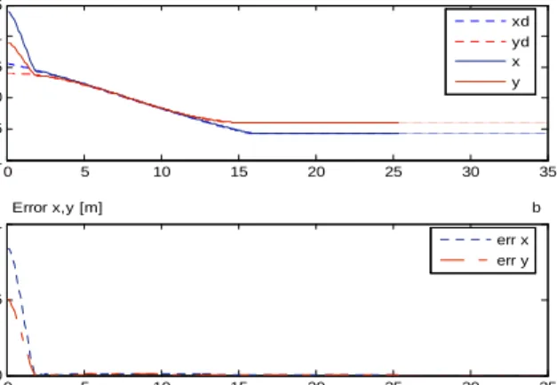
0 5 10 15 20 25 30 35 -1 -0.5 0 0.5 1 1.5 Posicion [m] a 0 5 10 15 20 25 30 35 0 0.5 1 Tiempo [s] Error x,y [m] b err x err y xd yd x y

Figure 7: x-y mobile robot states (a) and quadratic error (b)

From Fig. 7, it can be noticed the x-y position of

mobile robot and the quadratic error graphic, this error

tends to zero. 0 5 10 15 20 25 30 35 40 -0.2 0 0.2 0.4 0.6 0.8 Velocidad Lineal [m/s] a 0 5 10 15 20 25 30 35 40 -0.2 -0.1 0 0.1 0.2 Tiempo [s]

Velocidad Angular [rad/s] b w c w_real u c u real

Figure 8: Control actions (a) uc y (b) wc

Figure 8 shows control actions of system compared with real linear and angular speeds of mobile robot. It is observed that at the moment when mobile robot arrives to desire position, it is stayed there with null speed.

From Figs. 9(a) and 9(b), it is shown the execution time of optimization algorithm for each sampling time in the simulations.

Sequential algorithm is shown in Fig. 9(a), where 93%

of execution times are smaller than To, whereas

simultaneous algorithm is shown in Fig. 9(b), where

81% of execution times are smaller than To.

0 50 100 150 200 250 300 350 0 0.1 0.2 0.3 0.4

Tiempo del Algoritmo [s] a

0 100 200 300 400 500 600 700 0 0.1 0.2 0.3 0.4

Periodos de Muestreo [nTo]

Tiempo del Algoritmo [s] b

Figure 9: Algorithm execution time during simulation (a) sequential (93% < To), (b) simultaneous (81% < To)

V. CONCLUSIONS

The problem to lead a mobile robot through previous compute trajectories has been solved by using NMPC strategy like navigation algorithm. Dynamic holonomic model of unicycle-like mobile robot has been used; this model was validated by De la Cruz et al. (2006).

A good control system performance, by means NMPC has been achieved, both positioning and trajectory tracking. Results were obtained by using the NMPC sequential approach, because compute times with this algorithm were better than the NMPC simultaneous one, as it is observed in the simulations.

Proposed controller is able to implement experimentally as it is shown in the analysis of results. By using a suboptimal scheme, good results have been achieved; this proves that with specific software for this problem, it is possible to reach better results.

Simulations show that the most of NMPC compute times, are below the ranges accepted by mobile robot

(To = 0.1[s]), these simulations were done by using

MATLAB Optimization Toolbox. Furthermore,

preliminary compute times are highest due to the algorithm starts from distant initial conditions to the problem optimum.

Future works will entail a more robust analysis considering a nonzero uncertain vector and, in addition, experimental applications will be made in PIONNER mobile robots with collision avoidance techniques.

ACKNOWLEDGEMENTS

This work was partially funded by the Consejo Nacional de Investigaciones Científicas y Técnicas (CONICET - National Council for Scientific Research), Argentina and by the Servicio Alemán de Intercambio Académico (DAAD – Deutscher Akademischer Austausch Dients).

REFERENCES

Albagul A. y Wahyudi, “Dynamic Modeling and Adaptive Traction Control for Mobile Robots”,

Annual Conference IEEE IES, pp. 614-620, (2004).

Camacho E. y Bordons C., Model Predictive Control in

the Process Industry, Springer-Verlag, (1998). De la Cruz C. y Carelli R., “Linealización con

Realimentación del Modelo Dinámico de un Robot Móvil y Control de Seguimiento de Trayectoria”,

AADECA, (2006).

Dong W. y Kuhnert K., “Robust Adaptive Control of Nonholonomic Mobile Robot with Parameter and

Nonparameter Uncertainties“, IEEE Transactions

on Robotics, pp. 261-266, (2005).

Dongbing G. y Huosheng H., “Receding Horizon Tracking Control of Wheeled mobile Robots”,

Control Systems Technology, vol. 14, pp. 743-749, (2006).

F.A.C.C. Fontes, “A General Framework to Design Stabilizing Nonlinear Model Predictive

Controllers”, Sist. Control Lett., pp. 127-143,

(2001).

Hedjar R., Toumi R., Boucher P. y Dumur D., “Finite Horizon Nonlinear Predictive Control by the Taylor Approximation: Application to Robot Tracking

Trajectory”, Int. J. Appl. Math. Comp. Sci., vol. 15,

pp. 527-540, (2005).

Kanayama Y., Kimura Y., Miyazaki F. y Noguchi T., “A Stable Tracking Control Method for an

Autonomous Mobile Robot”, Proc. IEEE ICRA, pp.

384-389, (1990).

Künhe F., Gomes J. y Fetter W., “Mobile Robot Trajectory Tracking using Model Predictive

Control”, II IEEE LARS, (2005).

Mayne D., Rawlings J., Rao C. y Scokaert P., “Constrained Model Predictive Control: Stability and Optimality”, Automatica, pp. 789-814, (2000).

Peña M., Control basado en Modelos Borrosos, Tesis de

Doctorado – INAUT – UNSJ, (2002).

Ramírez D., Limón-Marruedo D., Gómez-Ortega J. y E. Camacho, “Aplicación del Control Predictivo basado en Modelo No Lineal a la Navegación de un Robot Móvil utilizando Algoritmos Genéticos”,

Métodos Numéricos en Ingeniería, (1999).

Secchi H., Control de Vehículos Autoguiados con

Realimentación Sensorial, Tesis de Maestría – INAUT – UNSJ, (1998).

Yang J. y Kim H., “Sliding Mode Control for Trayectory Tracking of Nonholonomic Wheeled

Mobile Robots”, IEEE Transactions on Robotics

and Automation, pp. 578-587, (1999).

Zhang Y., Hong D., Chung J. y Velinsky S., “Dynamic Model Based Robust Tracking Control of a Differentially Steered Wheeled Mobile Robot”,

Proceedings of the American Control Conference, pp. 850-855, (1998).