Learning to Control Linear Time-Invariant Systems with Discrete Time Reinforcement Learning

(1)

LEARNING TO CONTROL LINEAR TIME-INVARIANT SYSTEMS

WITH DISCRETE TIME REINFORCEMENT LEARNING

A Thesis by

ERIC JAMES NELSON

Submitted to the Office of Graduate and Professional Studies of Texas A&M University

in partial fulfillment of the requirement for the degree of MASTER OF SCIENCE

Chair of Committee, Thomas Ioerger Committee Members, Dylan A. Shell

John Valasek Head of Department, Dilma Da Silva

December 2016

Major Subject: Computer Science

(2)

ABSTRACT

Reinforcement learning (RL) is a powerful method for learning policies in environ-ments with delayed feedback in a model-free way. Another powerful method for obtaining control policies is the Linear Quadratic Regulator (LQR) problem, which utilizes knowl-edge of a linear model to derive the optimal policy. However, the continuously evolving dynamics of linear systems pose a challenge to using RL techniques as the underlying the-ory is discrete in nature. Therefore, reinforcement learners must discretize the dynamics by sampling at specific time intervals. The time interval used by the reinforcement learner directly affects the quality of the control policy that is learned. This work attempts to char-acterize the quality of learned policies as a function of the sample time of the reinforcement learner and in comparison with the optimal control as it is derived from the LQR frame-work. It is shown that in the limit as the sample time is decreased to zero, the policies generated converge to the optimal policies. In addition, any non-zero sample time intro-duces error into the learned policies. This error increases exponentially as a function of the sample time used to train the reinforcement learner.

(3)

(4)

ACKNOWLEDGMENTS

I would like to thank Texas A&M University, the Office of Graduate and Professional Studies, the Department of Computer Science and Engineering, and the faculty and staff for supporting me throughout my time here and giving me an opportunity to expand my knowledge.

I would also like to give a special thanks to Dr. Thomas Ioerger, whose passion, knowledge, and dedication helped me grow as both a graduate student and a person. With-out the dedication and support of Dr. Ioerger, this work would not have been possible.

(5)

NOMENCLATURE

RL Reinforcement Learning

CT Control Theory

LQR Linear Quadratic Regulator

LTI Linear Time Invariant

AOA Angle of Attack

MARE Matrix Algebraic Riccati Equation

CARE Continuous-time Algebraic Riccati Equation

HJB Hamilton-Jacobi-Bellman

RLS Recursive Least-Squares

(6)

LIST OF FIGURES

FIGURE Page

2.1 A depiction of the linear mapping (∆x=M(∆t)x(0) +L) for an input action for the example problem. Each vector shows the result of taking the same action from different coordinates in state space and holding it for∆t=0.2. . . 23 2.2 The optimal trajectory (red) and the discrete trajectory (blue), the optimal

trajectory is also plotted in x-space. The bottom right trajectory shows the shifted variable evolving inw-space. . . . 26 2.3 Differences between the optimal continuous-time trajectory and the

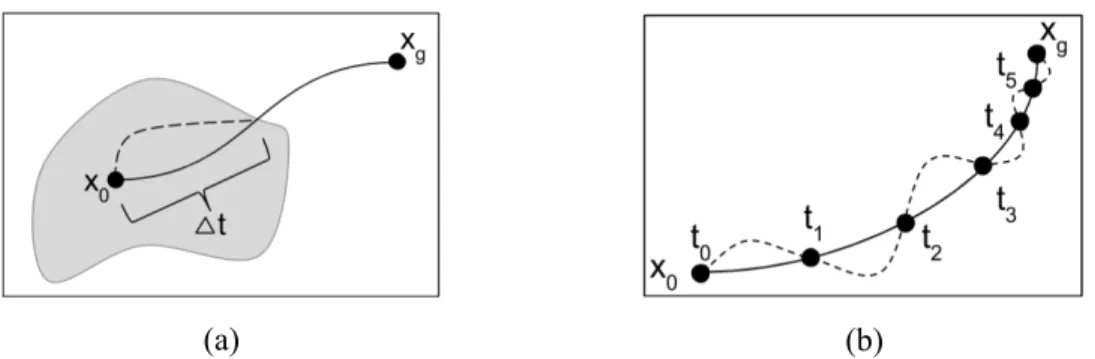
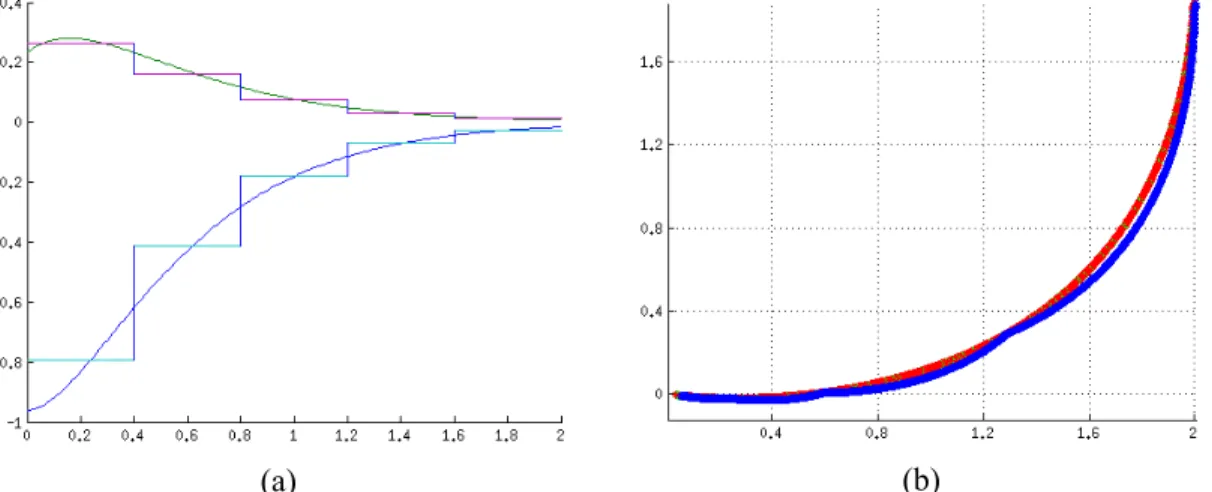
tra-jectory produced by a sequence of discrete inputs. Solid line shows continuous-time trajectory. The shaded region shows the reachable space within∆t. The dashed line shows trajectory by a sequence of con-stant inputs. . . 28 2.4 (a) Shows the discretization (∆t=0.4) between continuous and optimal

control inputs. The plot shows two different control inputs to the system over time. (b) Shows the path difference between following the discrete and continuous policies. . . 29 2.5 The value estimates from the learned policies as a function of∆t. . . . . 31 2.6 The bound (red) on the error vs. the true error (blue) for a single step

(sample time). The second figure shows the actual deviation between the discrete (blue) path and the optimal (green) paths. . . 36 2.7 The relationship between∆tand the maximum error of the example

prob-lem. . . 38 3.1 Depiction of the real-world longitudinal control problem. . . 41 3.2 The learned control makes jumps along the optimal trajectory

introduc-ing more error as the sample time increases. . . 43 3.3 The value estimates from the learned policies as a function of∆t for the

example system. The red line represents the optimal value and the blue line is the value estimate for the learned policy for a given∆t. . . . 44

(9)

3.4 The value estimates from the learned policies as a function of∆t for the Commander 700 system. The red line represents the optimal value and the blue line is the value estimate for the learned policy for a given∆t. . 45 3.5 The learned control must make changes in altitude in order to reach the

goal state. (a) shows the initial state of the aircraft. (b) shows aircraft at a level angle, but its velocity is lower than the goal. (c) shows control beginning to trade altitude in order to gain velocity. (d) shows the aircraft returning back to a horizontal flight path and reaching it’s goal. . . 46 3.6 The AOA of the Commander 700 over following the learned policy. . . 46 3.7 The single step error (blue) and its bound (red) for the example system

when the end state is exactly equal to a point on the optimal trajectory. . 47 3.8 The single step error (blue) and its bound (red) for the example system

when the end state is close to a point on the optimal trajectory. . . 47 3.9 The single step error (blue) and its bound (red) for the Commander 700

example. . . 48 3.10 The learned control is approximated with different sample times. There

are two control inputs for the example problem. The blue line shows the first input and the red line shows the second. The larger the sample time the worse approximation of the true continuous-time optimal value function. . . 50 3.11 The perceived errors plotted vs. sample time for the example problem. . 51 3.12 The perceived errors plotted vs. sample time for the Commander 700

problem. . . 52 3.13 The learned control is approximated with different sample times. There

are control input shown is the angle of the elevator on the Commander 700. The larger the sample time the worse approximation of the true continuous-time optimal value function. . . 53

(10)

LIST OF TABLES

TABLE Page

3.1 Error bound for different sample times and the actual perceived errors for the example problem. . . 49 3.2 Error bound for different sample times and the actual perceived errors

(11)

1 INTRODUCTION

Linear systems are ubiquitous in science and engineering. They are described by models derived from their physical properties and the equations describing their behavior. Often times, it is a goal for scientists and engineers to design controls in order to force the systems to behave in accordance to an objective function. There are two main methods for deriving such controls: control theory and reinforcement learning. The control theory method uses the model to analytically derive an optimal control. In contrast, reinforcement learning learns an optimal control through the use of a feedback signal which means a model is not necessary.

Reinforcement learning is beneficial in that it can learn a control in a model-free way. Typically, a reinforcement learning task is modeled as aMarkov Decision Process with discrete states and a set of discrete actions from which a learner can choose. When state-transition probabilities or reward functions are unknown a MDP becomes a reinforce-ment learning problem [1]. A typical reinforcereinforce-ment learner learns by starting in an initial state, taking an action, ending up in a new state, getting a reward, updating internal param-eters, and finally repeating. The goal of the reinforcement learner is to learn a policy that maximizes the long-term expected discounted reward.

Linear systems can represent a large number of physical phenomena (e.g. inverted pendula, vehicle dynamics, mixing in chemical vats). These systems are described through the physical equations governing them meaning the equations describing them are

(12)

inher-ently continuous in state, time, and control input. Linear systems are of particular interest in control theory (CT) due to the fact that there are well-studied methods for determining optimal or near optimal controls. However, unlike using reinforcement learning to control a system, these mechanisms require knowledge of the model.

Although these two subjects (RL and CT) are closely related there is a major dis-connect between the two as one is inherently continuous in time and the other inherently discrete. This disconnect introduces some interesting questions that will be answered in this work.

• Can a reinforcement learner learn to control a linear system?

• How close to optimal can the policy learned be? What should the sort of rewards should the learner be given?

• How often should a reinforcement learner sample the state and decide on a new action?

• How does the sample time from the previous question affect the control policy? • Is there a bound on the error for a given sample time?

1.1 Motivation

It is often the case that the true model of a system is not known and therefore it is useful to study the effect of using a reinforcement learner to learn to control such systems. When a digital controller is involved, there are limitations on how often the state of a system can be sampled. For example, the sample time is clearly limited by the cycle time

(13)

of the processor. An assumption of a step-input model is made in this work. That is, a control is selected by a reinforcement learner and it must be held for the entire sample time. Clearly, such a control is not as good as a continuously varying control input could be and therefore some cost will be incurred for any discrete sample time. This limitation is particularly critical to study for systems which rapidly change state. It is desirable to make this sample time as large as possible for a given system because cheaper hardware may be used or processing cycles can be saved. The goal of this work is to provide insight into the relationship between the selection of a sample time and quality of control.

1.2 Scope & Contribution

This work is only concerned with the control of linear systems. Non-linear systems present their own challenges and are often more difficult to analyze. However, there is no limitation placed on the order of the linear system in this work and some of the examples used are of higher order. The results only hold over the controllable subspace of the system. In other words, the goal cannot be to drive the system to an uncontrollable state.

In this work, it is shown that: a reinforcement learner can learn to control linear systems, the value function can be represented exactly through the use of a weighted set of basis functions, there exists a bound on the error produced from using a learned policy for a given sample time. The results have a real-world impact in that money or processing cycles can be saved though the intelligent selection of a sample time.

(14)

1.3 Previous Work

This work spurred from previous work done by Kenton Kirkpatrick, a previous doc-toral candidate at Texas A&M University [2]. He attempts to learn an optimal sample time adaptively by modifying the reinforcement learning algorithm and reward functions [3] [2]. He shows that it is possible to learn the best sample time from a set of sample times through this modification. This work differs from his in that it attempts to derive a theoret-ical description of the effects of the sample time that is not limited to a subset of possible sample times.

The reinforcement learning algorithms used in Kenton’s work are based on work by Bellman and his dynamic programming in which a problem is broken down into many sub-problems that must also be optimized [4]. Learning in the dynamic programming sense requires building an estimate of thevalue functionwhich assigns a value for being in a state and following a policy. The value assigned is the expected long-term reward for being in a statesand following a policyπ.

Vπ(s) =E_π[R(s)] =E_π[ ∞

∑

k=0 γk_r k+1] =R(s) +γ

∑

s′ Vπ(s′)

This representation of value requires knowing at least some model of the system in terms of the state transition function. Therefore, in order to factor out the state transition function, Q-learning was introduced by Watkins. In Q-learning, we learn a Q-function, instead of a value function, which assigns a value for being in a statesand taking an actiona.

Q∗(s,a) = (1−α)Q∗(s,a) +α[r+γmax

a′ Q

(15)

This factors out the need to know the state transition function and thus we can learn in a model free way [5].

Lagoudakis and Parr show that reinforcement learning can be done in continuous state spaces by representing Q-functions as a linear combination of a set of basis functions [ϕi...ϕN][6]. V(s) = N

∑

i wiϕi(s)

However, in this representation, the selection of the basis functions becomes the main issue and no general guidelines are given. This is likely due to the goal of generality in their work. They additionally show that policy iteration can be done with this representation of a value function using a least-squares weight updating technique.

Steven J. Bradtke’s work focuses on the convergence of reinforcement learning al-gorithms for LQR problems. These problems have the property that the optimizing control is represented as a linear feedback control.

u∗(t) =−Kx(t)

He shows that a recursive least squares update rule can be used to learn a Q-function [7]. However, he shows that it is possible for the algorithm to converge to a non-optimal Q-function in the LQR setting. This is due to the representation of the Q-Q-function as a linear combination over the basis set of the quadratic combination of state and control variables.

Q(s,a) = [ x u ] Hu [ x u]

(16)

representation of the Q-function so that the values in the cells of the tables can be incre-mentally updated. The question of what Q-function do we converge to can be answered by defining a fixed point to which the algorithm will converge.

[ x u]THu [ x u ] =x′Qx+u′Ru+γ[Ax+Bu a]Hu [ Ax+Bu a ]

This equation specifies (n + m)(n + m + 1)/2 equations with an equal number of unknowns. There are multiple solutions possible to this system of equations and therefore it is possible to converge to a non-optimal Q-function. However, Bradtke shows that the policy iteration algorithm he proposes that updates the weights on the set of quadratic basis and control variables by a Recursive Least Squares (RLS) update rule will converge to the optimal Q-function.

Brogan’s book Modern Control Theory describes solving the LQR problem in both continuous and discrete time [8]. In it, he also discusses the application of Pontryagin’s minimum principle and the minimization of the Hamiltonian as a necessary condition for optimality. These two ideas are used to derive the bounds on the error in this work.

Johnson et al. attempt to solve an N-player nonzero-sum game that is subject to continuous-time nonlinear dynamics [9]. Their solution is based on solving the Hamilton-Jacobi-Bellman equation that defines an optimality condition. Similar reasoning is used in this work in solving for optimal controls.

(17)

1.4 Background

Thissectionserves tointroduce thetopicsused inthe theoreticalsectionto derive results. Itservesasafoundationfortheother sections.

1.4.1 Linear Systems State-Space Representation

Modern control theory introduces the idea of the state of a system. In this repre-sentation, a set of state variables are chosen and the system is described by how these variables evolve over time. Any linear time-invariant (LTI) system withnstate variables, rinput variables, andmoutput variable can be written in terms of change in state by a set of simultaneous differential equations,

˙x(t) =Ax(t) +Bu(t)

y(t) =Cx(t) +Du(t)

where xis the state, y is the output anduis the control input. A is ann×nmatrix that describes the system dynamics. Bis ann×r matrix that describes how the inputs affect the change in state. C is an m×m matrix andD is an m×r matrix. We can solve the differential equation forxby employing the Laplace transform.

X(s) = (sI−A)−1x(0) + (sI−A)−1BU(s) (1.1)

then taking the inverse Laplace transform, x(t) =eAtx(0) +

∫ _t

0

(18)

Therefore, we can see that the internal behavior (state space trajectory) is not, in general, linear and instead the system evolves exponentially as a function of time. These trajectories have a transient phase of rapid response before slowing to a new equilibrium point which we call the long-term or asymptotic response. If we assume thatAis negative definite then as a control is applied, the exponential terms will approach zero as time passes. Eventually, the system will converge to a new equilibrium point as the exponential terms approach zero. Example

Consider the following linear system,

˙x(t) =         −1 2 0 −1 −4 1 0 0 −1         x(t) +         1 0 0 1 1 0         u(t)

The solution can be derived by using the Laplace transform. So we focus on the (sI−A)−1term first

(sI−A) =         s+1 −2 0 1 s+4 −1 0 0 s+1         (sI−A)−1=           2 s+2− 1 s+3 2 s+2− 2 s+3 − 2 s+2 + 1 s+3+ 1 s+1 1 s+3− 1 s+2 2 s+3− 1 s+2 1 s+2 − 1 s+3 0 0 1 s+1          

(19)

To solve forx(t)with x(0) =         1 0 1         and u(t) =     U1(t) U2(t)    

whereu(t)is a step function. We now have the parts to evaluate Equation 1.1. Multiplying the matrices out we can start to formulate the full solution in Laplace space,

(sI−A)−1x(0) =           1 s+1 0 1 s+1           and (sI−A)−1BU(s) =           1 s+1 2 s+2− 2 s+3 0 2 s+3− 1 s+2 1 s+1 0                1 s 1 s     =           − 1 s+1− 1 s+2+ 2 3(s+3)+ 4 3s 1 2(s+2)− 2 3(s+3)+ 1 6s 1 s− 1 s+1           Therefore, X(s) =           1 s+1 0 1 s+1           +           − 1 s+1− 1 s+2+ 2 3(s+3)+ 4 3s 1 2(s+2)− 2 3(s+3)+ 1 6s 1 s− 1 s+1          

(20)

so that x(t) =           e−t−e−t−e−2t+2 3e −3t₊4 3 1 2e −2t₋2 3e −3t₊1 6 e−t+1−e−t           =           −e−2t+2 3e −3t₊4 3 1 2e −2t₋2 3e −3t₊1 6 1           (1.3)

Solving for the Optimal Continuous Time Trajectory

Next, we need to find a policy u that optimizes some objective. The calculus of variations will prove to be useful in finding such a policy. Mathematically, we can describe the objective function as an integral of a cost function,

J=

∫ b a

f(x,y,y′)dx

where we want to find the function ythat minimizes J over the range[a,b] and satisfies initial and final boundary conditions. In this paper, we consider that the goal is to reach a target statex_d, and f(·)is the distance squared as a cost function, f =|xt−xd|2 or, for

generality, f =xTQxin matrix form, whereQis a matrix of weights. Using Calculus of Variations, a necessary condition for an extremum function is that it satisfies the Euler-Lagrange equation. ∂f ∂y− d dx ( ∂f ∂y′ ) =0

The optimal control for a given objective function can be found in a similar manner. This will correspond to how we find an optimal policy in the case of continuous state spaces. For example, take the objective function [8]

J=

∫ tf

(21)

First we define the pre-Hamiltonian H(x,u,p,t) =L(x,u,t) +pT(t)f(x,u,t) ˙ p=∂H ∂x H=xTQx+uTRu+pT(Ax+Bu)

Pontryagin’s minimum principle specifies that the optimal policy is one that minimizes the Hamiltonian at every timet[8]. The Hamiltonian for this example is minimized by setting

∂H ∂u =0=2Ru+p T B u∗(t) =−1 2R −1_BT_p(t)

wherep(t)is the co-state vector that can be solved for through the use of boundary con-ditions. This gives us the optimal continuous time policyu∗(t)that minimizesJ. Further-more, the optimal continuous-time trajectory can be derived as:

˙x(t) =Ax(t) +Bu∗(t) ˙x(t) =Ax(t)−BKx(t)

x(t) =e(A−BK)tx(0)

whereK=R−1BTP

1.4.2 Solving for the Optimal Continuous Time Value Function

One can solve for the optimal value function by solving the Hamilton-Jacobi-Bellman (HJB) equation [9]. If we define the value function as

V =

∫ _∞

0

(22)

whereQandRare positive definite matrices. Then we can define a differential equivalent [10]

0=r(x,u) +∇VTx˙ The RHS of this equation is the Hamiltonian of the system.

H(x,u,∇V) =r(x,u) +∇VTx˙ and we arrive at

0=min

u H(x,u,∇V)

which is the HJB equation.

If we assume that the value function is a quadratic function in the Euclidean dis-tance to the origin then we can derive an analytical solution for the value function based on solving the Matrix Algebraic Riccati Equation (MARE) equation ATP+PA+Q+ PBR−1BTP=0[10]. V(x) =xTPx P= ∫ _∞ 0 etATQetAdt

wherePis the solution to the MARE equation. Note that the integral in the definition ofP doesn’t need to be solved directly. Instead,Pis the solution of then(n+1)/2simultaneous equations defined by the MARE equation. Also, note that these results only hold if the origin is the goal. Therefore, if the goal is to control the system to a target equilibrium point,xd, that is not at the origin, then a change of variables where the new origin is defined

(23)

asw=x−xd can be carried out using the chain rule dw dt =w˙ = dw dx dx dt =Ax+B(U+∆u) ˙ w=Aw+Axd+BU+B∆u=0 ˙ w=Aw+B∆u whereU=−B−1Axd. 1.4.3 LQR Problem

The LQR is a special class of control problems that are well studied. The assumptions for this problem in this work are as follows:

1. Continuous LTI dynamicsx˙=Ax+Bu

2. Infinite horizon (minimize objective ast→∞)

3. Deterministic (i.e. No probabilistic transitions or noise) 4. The goal must be to regulate to the origin (xd=0)

If this is not the case, then we can change variables (see Section 1.4.2).

5. The system is controllable. A system is controllable if the controllability matrixR has full row rank.

R= [B AB A2B ··· An−1B]

Given those assumptions, we define an objective function that we would like to minimize, J=

∫ _∞

0

x(t)TQx(t) +u(t)TRu(t)dt

(24)

equa-tion, the objective function is minimized by selecting the control u(t) =−R−1BTPx(t)

meaning that the minimal cost to get to the goal fromx(0)is V =x(0)Px(0)

wherePis the solution to the Continous-time Algebraic Riccati Equation (CARE). 1.4.4 Reinforcement Learning

Reinforcement learning (RL) is a method of machine learning in which an agent learns a control policy by attempting to maximize the returned rewards for taking an action in a given state [11]. It does this by exploring the state and action spaces and observing the rewards in order to approximate thevalue functionwhich is the expectation of the sum of discounted rewards for starting in state s and following the policy π. An important assumption made by the RL framework is that state changes are discrete; when an action is taken, a transition to a new state occurs, and the reward is observed, instead of happening continuously in time. If the value function is known, the optimal policyπ∗can be derived as:

π∗(s) =arg max

s′

V(s′)

Markov Decision Processes

Much of the theory of reinforcement learning is based on what are calledMarkov Decision Processes (MDPs) [1]. A MDP is defined on a set of states S and actions A available to an agent. The size of the state and action spaces are traditionally assumed to

(25)

be finite. The reward function R(s,a) defines the feedback given to the agent for being in state s, taking action a, and ending in state s′. Actions can either be deterministic or non-deterministic. If the current state depends only on the previous state and action taken then the problem is said to satisfy theMarkov property. Given this definition of an MDP, we now define the value function for a given policy (mapping of states to actions)π as

Vπ(s) =E_π[R(s)] =E_π[ ∞

∑

k=0 γk_r k+1]

Whereγis adiscount factorthat tunes how much the agent should care about future rewards versus the current reward. In other words, the value of being in state s is equal to the expected value of sum of the current reward and all future rewards for being in state s and followingπ until termination.

If the reward and transition functions are known, an MDP can be solved by em-ploying dynamic programming techniques [4]. Value iteration is one such technique in which one can iterate on the value function by taking the max over the actions V(s) = max a ∑_s′P a ss′ [ Ra ss′+γV(s′) ]

. The iterations continue until the LHS of the equation is equal to the RHS. The equation above is called the Bellman equation, which is based on the Bellman Principle of Optimality.

Q-learning

Some typical methods of reinforcement learning, such as the value iteration algo-rithm, require the learner to know some model of the underlying system (i.e. the reward function or state-transition function). However, it is often the case that one does not know these functions. Q-learning can be used to learn policies without having to know a-priori

(26)

the reward or state-transition functions. Instead of a value function, we now define a Q-function that represents the value of being in statesand taking actiona

Qπ(s,a) =E_π[R(s,a)] =E_π[ ∞

∑

k=0 γk_r k+1]

The Q-function is typically represented as a table called a Q-table where the rows and columns are the finite states and actions. Q-learning can be extended to infinite state spaces by representing Q-functions as the sum of weighted basis functions

ˆ Q(s,a) = N

∑

i=1 wiϕi(s,a)

This representation requires choosing a set of basis functions,ϕi(s,a), that can accurately

represent the true value function for a given problem. Algorithm 1Q-learning algorithm.

1: functionQlearn(Q)

2: Q=Q0=initial guess

3: fori←1to∞do

4: s=new random state

5: whilesis not terminaldo

6: Choosea(randomly,ε-greedy, etc.)

7: Observer,s′ 8: Q(s,a) = (1−α)Q(s,a) +α[r+γ(maxaQ(s′,a))] 9: end while 10: end for 11: end function Policy Iteration

Given an initial policyπ0one can find an optimal policy by performingpolicy itera-tion. In policy iteration, the value function for the current policy is solved for or estimated. Next, the policy can be improved by checking if at every state we can change an action

(27)

that improves the overall value. This leads to a new policy that can be used in the value function estimation step. These iterations can continue to be done with the guarantee that the policy is improving at each step. See Algorithm 2.

Algorithm 2Policy Iteration algorithm.

1: functionPolicyIteration(N,M,π0) 2: π=π0 3: fori←1toNdo 4: Vπ =PolicyEval(π,M) 5: π =PolicyUpdate(Vπ) 6: end for 7: returnπ∗ 8: end function

Adaptive Policy Iteration

The policy iteration algorithm used in our experiments was proposed by Steven Brad-kte in his work on using reinforcement learners on LQR problems [7]. In this algorithm, one updates the estimate of the true Q-function by adjusting weights through a Recursive Least-Squares (RLS) update rule. Given the value function for a policyU is represented as

VU(xt) =xt′KUxt

and the single-step reward function is represented as rt =x′Qx+u′Ru

Updatingθ_kcan be accomplished through the following two equations

θk(i) =θk(i−1) +

Pk(i−1)ϕt(rt−ϕt′θk(i−1))

(28)

Algorithm 3Adaptive Policy Iteration (API) algorithm. 1: functionAPI(N) 2: θ =θ0=initial guess 3: fork←1to∞do 4: Pk=P0 5: fori←1toNdo 6: ui=Ukxi+ei 7: xi=rk(xi,ui) 8: Updateθkusing RLS 9: end for 10: UpdateUk based onθk 11: θk+t =θk 12: end for 13: end function Pk(i) =Pk(i−1)− Pk(i−1)ϕtϕt′Pk(i−1) 1+ϕ_t′P_k(i−1)ϕt

In addition, updatingU_k can be accomplished through the following equation Uk+1=−H_U−_k1₍₂₂₎HUk(21) where Hk=     Q+γA′KuA γA′KuB γB′KuA R+γB′KuB    

An exploratory signal et that is persistently exciting is necessary in order to ensure

con-vergence of the value function. In this work, like Bradkte suggests, a random signal from a normal distribution is used as it performed well in experiments. Although, such an ex-ploratory signal doesn’t satisfy the persistent excitation condition.

(29)

2 ANALYSIS

&

THEORY

*

2.1 LTI System Behavior

This section will discuss how the behavior of a linear system can be decomposed into a transient and long term portions which represent how the system behaves in the short term after an action is taken and where the system will converge to.

2.1.1 Decomposition

In this section, we prove that a given linear system can be decomposed into a linear function of the transient and long term behaviors of the system.

Theorem 2.1 IfAhas bothrealand distincteigenvalues, then each entry in the solution to the state equation (Eq. 1.2) can be written as the sum of exponentials and constants.

Recall the solution to the state space equations in the Laplace domain given by Equation 1.1. Note thatx(0)andBare both constant andU(s)is a step input. Therefore, let us focus on the(sI−A)−1term first. Using|sI−A|=0, we can obtain the eigenvalues ofA, which we assume by the theorem are both real and distinct. We can write

|sI−A|= (s−λ1)(s−λ2)...(s−λn) (2.1)

*Portions of this section are reprinted with permission from “Learning to Control First Order Linear SystemswithDiscreteTimeReinforcementLearning”byNelson,E.Ioerger,T.R,2016.Proceedingsofthe 2016InternationalConferenceonEmbeddedSystems,Cyber-physicalSystems,&Applications,pp.

(30)

which is a polynomial of degree n. LetMi j be the matrix obtained by eliminating the ith

row and jthcolumn fromA. |Mi j|is called the minor ofai jand has a degree≤(n−1). Let

Ai j = (−1)i+j|Mi j| (2.2)

be called the cofactor ofai j. The adjoint ofAis the matrix in which

ad j(A)i j =Aji (2.3)

In other words, the adjoint ofAis the transpose of the matrix of cofactors. Since (sI−A)−1= ad j(sI−A)

|sI−A| We can use Eqs 2.1, 2.2, and 2.3 to write

ad j(sI−A)i j (s−λ1)(s−λ2)...(s−λn) = (sI−A)ji (s−λ1)(s−λ2)...(s−λn) = (−1) j+i_|_M ji| (s−λ1)(s−λ2)...(s−λn)

Because the degree of|Mji| is at most(n−1) the degree of the numerator is strictly less

than the degree of the denominator.

Therefore, we can use partial fraction decomposition since there are no repeated roots in the denominator and the degree of the numerator is strictly less than the degree of the denominator to get the form

k1 (s−λ1) + k2 (s−λ2) +...+ kn (s−λn)

Finally, taking the inverse Laplace transform we get: k1eλ1t+k2eλ2t+...+kneλnt

(31)

for each entry in(sI−A)−1as shown below. (sI−A)−1=             k111eλ11 t₊_...₊_k n1neλ1n t k121eλ 21t₊_...₊_k n2neλ1n t .. . k1n1eλn1 t₊_...₊_k nnneλ1n t            

Sincex(0)is a vector of constants for the first half of equation 1.1 we get

=             c1k111eλ11 t₊_...₊_c 1kn1neλ1n t c2k111eλ 11t₊_...₊_c 2kn1neλ 1nt .. . cnk111eλ11 t₊_...₊_c nkn1neλ1n t             For the second half of equation 1.1, we have two parts

(sI−A)−1B=             b1k111eλ11 t₊_...₊_b 1kn1neλ1n t b2k111eλ11 t₊_...₊_b 2kn1neλ1n t .. . bnk111eλ11 t₊_...₊_b nkn1neλ1n t             For the unit step in each dimension ofU(s)

U(s) = 1 sK T₌ [ k1 s k2 s ··· kn s ]T

we take the inverse Laplace transform to get

U(t) =U=KTH(t)

(32)

the matrix for(sI−A)−1BU. Therefore,

x(t) =L−1((sI−A)−1x(0) + (sI−A)−1BU(s)) =L−1(sI−A)−1x(0) +L−1(sI−A)−1BU(s)) =

            C1k1₁₁eλ11t₊_...₊_C1k n1neλ1n t C2k121eλ21 t₊_...₊_C 2kn2neλ2n t .. . Cnk1n1eλn1 t₊_...₊_C nknnneλnn t            

whereCi=ki(bi+ci)andiis equal to the row index. Therefore, as long as the eigenvalues

of the matrixAare bothrealanddistinctthe solution to the state equation can be written as a sum of exponential functions and constants.

If we group the exponential terms together, they form what we call the transient response matrix T of the system. The constants form the long term response matrix N of the system. The λ terms in the transient response matrix are the time constants of the system. We can now define

x(t) =T(t) +N

For the example problem in section 1.4.1, separating exponentials from constants in equa-tion 1.3, we have T =           −e−2t+2 3e −3t 1 2e −2t₋2 3e −3t 0           , N =           4 3 1 6 1          

(33)

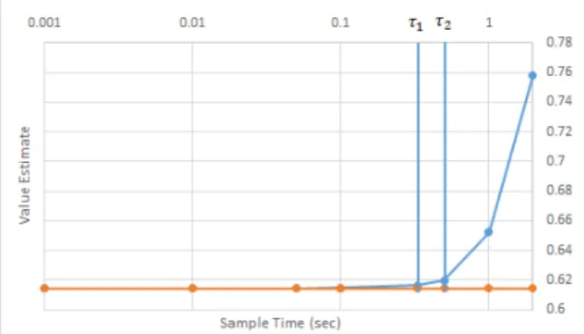
The smallest time constant is given byτ = 1₃. Thus, the system reaches about 37% of the way to the new equilibrium point

[ 4 3 1 6 1 ]T in about 1/3 sec.

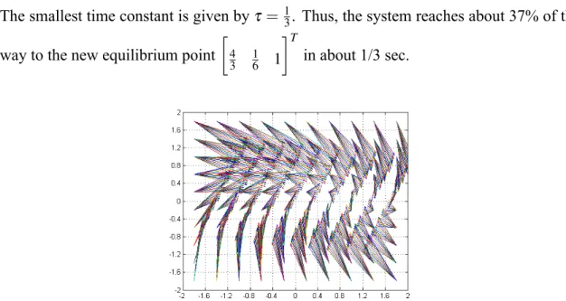
Figure 2.1: A depiction of the linear mapping (∆x=M(∆t)x(0) +L) for an input action for the example problem. Each vector shows the result of taking the same action from different coordinates in state space and holding it for∆t=0.2. [12]

Assuming the step-function input model, for a given∆tthe response is linear ∆x=M(∆t)x(0) +L

as shown in Figure 2.1.

2.2 Reinforcement Learning for the LQR Problem

In reinforcement learning, it is important that the states exhibit the Markov property as defined in Section 1.4.4 as the underlying theory relies on this assumption. We claim that the Markov property holds in the context of the LQR problem.

Theorem 2.2 Continuous LTI systems that are sampled at a given rate (∆t) exhibit the Markov property.

(34)

In order to prove this, we need to show that the next state is dependent only on the current state and action. A discretized version of the system can be defined with the introduction of a∆t Xk+1=Adxk+Bduk where Ad=eA∆t Bd= [∫ _∆t 0 eAτ dτ ] B

Using these definitions it can be clearly seen that the next state is only dependent on the current state (xk) and the current action (uk). Therefore, the LQR systems in this work

exhibit the Markov property.

Assuming the objective function that we want to minimize is defined as V =

∫ _∞

0

x(t)TQx(t) +u(t)TRu(t)dt

Then, we know from the LQR theory, which is based on Lyapunov theory, that the value function can be represented as [13] [7] [12]

V∗(x) =xTPx The proof is as follows.

The HJB equation is defined as 0=min u [x ′_Qx₊_u′_Ru₊_∇_VT_(Ax₊_Bu)] tryingV =x′Px 0=min u [x ′_Qx₊_u′_Ru₊_PxAx₊_PxBu]

(35)

now we take the partial over u in order to minimize 0=2Ru+BTPx u(t) =−1

2R

−1_BT_Px(t)

Therefore, a solution to the HJB equation and therefore an optimal control isu=−Kx(t) which means that the value function is represented as:

V =x′Px

In addition, this work uses a weighted set of basis functions to represent the Q-function that is being learned. It has been shown that the Q-Q-function for the LQR problem can be directly represented as a linear function over the quadratic set of state and control variables of the system [7]. That is,

Q(s,a) = [ x u ] Hu [ x u]

How do we update the weights on the set of quadratic variables? By defining the reward for each episode as

rt= x(t_| )T_{zQx(t)_}

Penalize distance to goal

+ u(t)TRu(t) | {z } Penalize magnitude of control

= (x−xd)2+u2 (2.4)

Assuming, for simplicity, that Q=R=I. Note that although this might seem like the learner is being given copious amounts of information, it is just a number as given in many other reinforcement learning tasks. In addition, the reward is at a single point in time which is distinct from the value function which represents following a policy from a given state and accumulating the rewards along the whole path.

(36)

Q-functions. Using the approximate Q-functions, policy iteration can be done. The benefit of following such an algorithm is that the state and action spaces can be continuous and no discretization is necessary [7].

2.2.1 Change of Variables

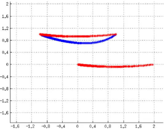
The value function as defined in Section 2.2 is based on the origin being the desired goal of the system. That is, Qmust be quadratic around the origin. If this is not the case, then it is necessary to perform a change of variables in order to shift the origin to the desired position in state-space. Figure 2.2 shows the shifted optimal trajectory caused by changing variables.

Figure 2.2: The optimal trajectory (red) and the discrete trajectory (blue), the optimal tra-jectory is also plotted in x-space. The bottom right trajectory shows the shifted variable evolving inw-space.

Therefore, if the goal is to control the system to a target equilibrium point,xd, that is

not at the origin, then a change of variables where the new origin is defined asw=x−xd

can be carried out using the chain rule, as was shown in Section 1.4.1,

dw dwdx

(37)

˙

w=Aw+Axd+BU+B∆u=0

˙

w=Aw+B∆u

whereU=−B−1Axd. In words, this means that in order to get a new equilibrium point we

must input a constant control that shifts the system to that new equilibrium. It should also be noted that the system must be controllable in order to ensure that such a control exists.

2.3 Effect of Sample Time

If we assume continuous control inputs that are bounded by some constant µ (i.e. |U| ≤ µ) then areachable region from the current state is defined given a ∆t. This is illustrated in Figure 2.3 as the light gray region. A statex2is said to bereachablefromx1 if there exists a control inputu(t)such that|u(t)|<µ that can transfer the system fromx1 tox2in finite amount of time. It should be noted that the shape of the region is dependent on the dynamics of the system and is not necessarily circular. The optimal trajectory, x∗(t), is represented as the solid black line in the figure and a constant input trajectory for a given action is shown as a dotted line. The dotted line represents choosing an action and holding it constant for∆t. It is curved because of the non-linear, transient response of the system. There is always a constant action that can move the system to the same point on the continuous time trajectory after∆t.

(38)

(a) (b)

Figure 2.3: Differences between the optimal continuous-time trajectory and the trajectory produced by a sequence of discrete inputs. Solid line shows continuous-time trajectory. The shaded region shows the reachable space within∆t. The dashed line shows trajectory by a sequence of constant inputs. [12]

Theorem 2.3 The constant control chosen by the optimally, converged learner will be one which minimizes the Hamiltonian, and this control will be a constant step input which causes the state trajectory to intersect with the optimal continuous-time trajectory after∆t.

This can be proven using the ideas from Pontryagin’s Minimum Principle and Bell-man’s optimality equation. Pontryagin’s Minimum Principle states that the optimal policy is the one which minimizes the control Hamiltonian at every timet along the optimal tra-jectory.

H(x∗(t),u∗(t),λ∗(t),t)≤ H(x∗(t),u(t),λ∗(t),t), ∀u∈ U

and Bellman’s optimality equation describes the optimal value function, V∗(s) =min

a R(s,a) +γV

∗₍_T_(s_,_a))

The optimal value function can be derived by following the optimal trajectory as described by Pontryagin’s Minimum Principle as following the optimal control policy in continuous time leads to the optimal value at every timet. The inner portion of Bellman’s optimality

(39)

equationR(s,a)+γV∗(T(s,a))is minimized by choosing the actionasuch that it intersects with the optimal trajectory after ∆t. Therefore, the optimal action for the reinforcement learner to choose would be the one which causes the state to intersect with the optimal trajectory after∆t. This proof assumes that the under the learned value function is equal to the optimal value functionV∆t=V∗while it is not strictly guaranteed that this is true, we show that as ∆t →0 the learned value function approximates the optimalV∆t ≈V∗. Therefore, this assumption holds for reasonable selections of∆t.

(a) (b)

Figure 2.4: (a) Shows the discretization (∆t=0.4) between continuous and optimal control inputs. The plot shows two different control inputs to the system over time. (b) Shows the path difference between following the discrete and continuous policies.

Next, we show that in the limit as∆t→0, we get better control policies. For a smaller ∆t, the reachable region is smaller which implies the maximum distance away from the optimal trajectory is also smaller. The error of the policy for a given∆t is defined by the difference of the integral of the distance to the goal for the trajectories produced by both policies. An example approximation of an optimal policy and trajectory is shown in Figure

(40)

2.4.

An important goal is to show that the value function learned by reinforcement learn-ing will converge in the limit (as∆t→0) to the optimal value function for continuous time control,

Q∗=

∫ _∞

0

(x(t)−xd)T(x(t)−xd) +uTu dt

Although the discrete-time value function is conventionally defined as the expected long-term discounted sum of rewards (i.e. V =Σγirt), in order to get it to converge toV∗, we

modify by settingγ =1and multiply by∆t,

V_∆t=∆t Σ∞t=0rt=∆t Σt=∞0(x(t)−xd)T(x(t)−xd)

We are able to setγ=1because we are only considering controllable systems which means that as the system evolves the rewards will approach 0 and therefore a discount factor is not necessary for convergence.

Since for any time step∆t, there is always a constant action that can move the system to the same point on the continuous time trajectory, as proven above, then the rewards rt= (x(t)−xd)T(x(t)−xd) +uTuwill match at these discrete points. Thus, the discrete-time value function is simply the numerical approximation of the continuous-discrete-time value function,Q∗. Q∗= ∫ _∞ 0 (x(t)−xd)T(x(t)−xd) +uTu dt≈Σ∞t=0∆t [ (x(t)−xd)T(x(t)−xd) +uTu ] lim ∆t→0Q∆t →Q ∗

(41)

Figure 2.5: The value estimates from the learned policies as a function of∆t.

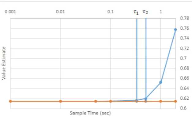
Furthermore,wecanweputaboundontheerrorinthevaluefunction. Theerrorisa functionofthetimestepsize(aswithanynumericalquadrature),aswellasthemaximum deviationbetweentheoptimalcontinuous-timetrajectoryandtheconstant-inputtrajectory betweenthediscretetimepoints,wherethecoordinatescoincide. Thisisboundedbecause theamounttheconstant-inputtrajectorycandivergefromthecontinuoustimepathwithin ∆tislimitedbythedynamicsofthesystem,whichwillforcethemtofollowsimilarpaths. These ideas are illustrated in Figure2.5, the points along the curveshow different ∆t’s thatwere usedtotrain areinforcementlearneruntilconvergence. Thetime constantsof eachoftheexamplesystemaremarkedasverticallines.Theexamplesystemisdiscussed further throughout Section 3. It can be seen thatthe value approaches the optimal value asymptoticallyas∆t→0. Thevalueestimatesarecostforreachingthegoal(i.e.thelower thebetter).

The response to a given input, and therefore the error, is dependent on the underlying system dynamics, and it is also dependent on how quickly a system responds to a new input. The smallest system time constant, τ, defines how rapidly the system responds to a new

(42)

control input. Therefore, we propose that a requirement for the selection of a ∆t is that it be less thanτ in order to ensure that these rapid responses can be controlled. At∆t =dt the optimal trajectory will equal the approximate trajectory through state space.

2.3.1 Bounding the Single-step Error

The goal of bounding the total path error can be obtained by first quantifying the error for a single step of holding a control for a given sample time. Given Theorem 2.3, we know that the optimal continuous and the discrete trajectories should converge to some point along the reachable region. Therefore, the single-step error is bounded by the dynamics of the system.

Theorem 2.4 The error introduced by a single discrete stepd(t)is bounded above by d(t)≤t∥BK∥eµ(A)+∥BK∥t−[eAt−I][∆t∥BK∥eµ(A)+∥BK∥∆t]∥x(0)−xd∥

In order to derive the error bound mathematically, we start with the fact that we know the optimal control policy for the infinite-horizon, continuous-time Linear Quadratic Regulator (LQR) objective function

J= ∫ tf 0 w(t)TQw(t) +u(t)Ru(t)dt (2.5) which is u=−Kw=−K(x−xd) =−Kx+Kxd (2.6)

whereK=BTPandPis the solution to the Continuous Time Algebraic Riccati Equation (CARE). Plugging into the dynamics we get

(43)

˙

w= (A−BK)w w=e(A−BK)tw(0) x−xd =e(A−BK)t(x(0)−xd)

meaning the optimal trajectory is defined as

x(t) =σ∗(t) =e(A−BK)t(x(0)−xd) +xd (2.7)

The discrete time trajectory is defined as (from [14])

w(t) =eAtw(0) +A−1[eAt−I]BL x(t)−xd=eAt(x(0)−xd) +A−1[eAt−I]BL

x(t) =σ(t) =eAtx(0)−eAtxd+A−1[eAt−I]BL+xd (2.8)

whereLis a constant input that causes the system to end in the same state as the optimal trajectory after∆t. Lcan be derived by

σ∗(∆t) =σ(∆t) e(A−BK)∆t(x(0)−x_d) +x_d=eA∆t(x(0)−x_d) +A−1[eA∆t−I]BL+x_d e(A−BK)∆t(x(0)−xd)−eA∆t(x(0)−xd) =A−1[eA∆t−I]BL [ A−1[eA∆t−I]B ]₋1[ e(A−BK)∆t(x(0)−xd)−eA∆t(x(0)−xd) ] =L L= [ A−1[eA∆t−I]B ]−1[ e(A−BK)∆t(x(0)−xd)−eA∆t(x(0)−xd) ] (2.9)

With these definitions, we can define the difference between trajectories as d(t) =σ∗(t)−σ(t)

(44)

d(t) = [ e(A−BK)t(x(0)−x_d) +x_d ] −[eAt(x(0)−x_d) +A−1[eAt−I]BL+x_d ]

d(t)is related to the error in the value function via the triangle inequality in that the distance between both trajectories is bounded above by the distance to the goal from the optimal trajectory. That is,

ε =V_∆t−V∗ = ∫ _∞ 0 V_∆t(x(t))− ∫ _∞ 0 V(x∗(t))dt = ∫ _∞ 0 V_∆t(x(t))−V(x∗(t))dt = ∫ _∞ 0 (x(t)−xd)2−(x∗(t)−xd)2dt

By the triangle inequality,

≤∫ ∞ 0 (x(t)−x∗(t))2dt ε≤∫ ∞ 0 (d(t))2dt Continuing by plugging inL, we get,

= [ e(A−BK)t−eAt ] (x(0)−xd)− [ A−1[eAt−I]B ][ A−1[eA∆t−I]B ]−1 C [ e(A−BK)∆t−eA∆t ] D (x(0)−x_d) = [ e(A−BK)t−eAt ] (x(0)−x_d)− [ A−1[eAt−I]B ] CD(x(0)−x_d) d(t) = [[ e(A−BK)t−eAt ] part1 −[A−1[eAt−I]B ] CD part2 ] (x(0)−xd) (2.10)

Mathematically, the error bound can be derived by first defining the logarithmic norm,

µ(A) = lim

h→0+

(∥I+hA∥ −1) h

(45)

In contrast to the previous definition, we need to redefine d(t). Specifically, we need to take the norm in the definition ofd(t),

d(t) =[e(A−BK)t−eAt]−[eAt−I][eA∆t−I]−1[e(A−BK)∆t−eA∆t]∥x(0)−x_d∥ We can then continue to derive a bound by approximating

[eAt−I][eA∆t−I]−1≤[eAt−I]

d(t)≤[e(A−BK)t−eAt]−[eAt−I][e(A−BK)∆t−eA∆t]

A convenient bound for the perturbation of exponential matrices is defined as [15]

e(A−BK)t−eAt≤t∥BK∥eµ(A)+∥BK∥t

where µ(A)is the logarithmic matrix norm as defined above. Using this bound we can conclude that

d(t)≤t∥BK∥eµ(A)+∥BK∥t−[eAt−I][∆t∥BK∥eµ(A)+∥BK∥∆t]∥x(0)−xd∥

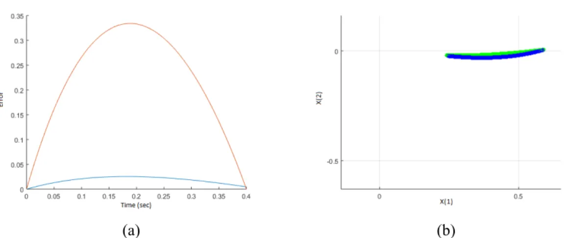
An example of this bound can be seen in Figure 2.6 using the following dynamics,

A=     −1 2 −1 −4    B=     2 −1    P=     0.2917 0.0833 0.0833 0.1667    K= [ 0.5 0 ] with a∆t=0.63

(46)

(a) (b)

Figure 2.6: The bound (red) on the error vs. the true error (blue) for a single step (sample time). The second figure shows the actual deviation between the discrete (blue) path and the optimal (green) paths.

2.3.2 Bounding the Total Path Error

Theorem 2.5 The error introduced by a∆t(ε) over the whole path to the goal is bounded above by

ε ≤Ψ∥(A−BK)∥C∥(x(0)−xd)∥∆t

1−e−α∆t The single time step path error,

d(t)≤t∥BK∥eµ(A)+∥BK∥t−[eAt−I][∆t∥BK∥eµ(A)+∥BK∥∆t]∥x(0)−xd∥

can be used to derive a bound on the total errorε. The maximum of the first norm ind(t) can be defined as

Ψ=∆t∥BK∥e(µ(A)+∥BK∥∆t) which leaves us with

(47)

ε≤

∑

∞ i=0 d(∆t·i) ε ≤

∑

∞ i=0 Ψ∥x(∆t·i)−x(∆t·(i+1))∥

Assuming that the system is stable, the maximum difference between ∥x(∆t·i)−x(∆t·(i+1))∥is bounded above byx(˙ ∆t·i)∆t becausex(i)will be decreasing exponentially toward0inwspace asi→∞. Using this we get

ε ≤Ψ

∑

∞

i=0

(A−BK)e(A−BK)∆ti(x(0)−xd)∆t

where x(0) andxd are the overall start position and the overall goal for the whole path,

respectively.

One important property of matrix norms is

∥AB∥ ≤ ∥A∥∥B∥

for square matricesAandB. Using that property we can modify the definition ofε,

ε ≤Ψ

∑

∞ i=0 ∥(A−BK)∥e(A−BK)∆ti(x(0)−xd)∆t ε ≤Ψ∥(A−BK)∥ ∞

∑

i=0 e(A−BK)∆ti(x(0)−xd)∆t ε ≤Ψ∥(A−BK)∥ ∞

∑

i=0 e(A−BK)∆ti∥(x(0)−xd)∥∆t

One final issue that we must deal with is the infinite sum in the definition ofε. First, the inner term of the norm

(48)

is bounded by

e(A−BK)∆ti≤ ∥P∥eJP−1≤Ce−α∆ti whereC=∥P∥P−1andα =−max

λi

ℜeig(A−BK).

After substituting we see that this can be formulated as a geometric series,

∞

∑

i=0 Ce−α∆ti= ∞

∑

i=0 C ( ₁ e−α∆t )i = C 1− ( ₁ eα∆t ) Therefore, we arrive at the final bound

ε ≤Ψ∥(A−BK)∥C∥(x(0)−xd)∥∆t

1−e−α∆t

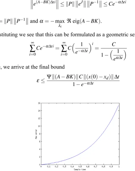
Figure 2.7: The relationship between∆t and the maximum error of the example problem.

Therefore, it can be seen that the maximum amount of error introduced is exponen-tially related to the∆tused to learn a control for a given system. This can be seen in Figure 2.7 where the dynamics of the system for the plot are defined by

A=     −1 2 −1 −4     andB=     2 −1 −1 1    

(49)

3 EXPERIMENTS

3.1 Verification

In order to test the bound and the theory in this work two main systems are defined: a simple theoretical system that adheres to the assumptions of stability and controllability and a real-world system that can be linearized in order to run in the simulator discussed below. With the systems defined, the first focus is to show that the single-step error bound holds by running single steps in both the real-world and example systems. Therefore, a learner will be trained until convergence on each system and the error bounds for each single step along the path will be compared to the perceived error. Building on the single-step error is the next single-step, the full-path error will be analyzed for both the example and real-world systems in a similar fashion to the single-step error. In addition, for both of the systems, it will be important to show that in the limit as∆t→0the value function learned approaches the optimal:V∆t→V∗. Therefore, a random initial state can be chosen and the policy for each ∆t can run until the goal is reached. The accumulated cost for following each policy will then be plotted in order to show the relationship between∆tand the value for using a specific policy.

The learning algorithm used in these examples is the adaptive policy iteration algo-rithm proposed by Bradtke in his work on applying reinforcement learning to LQR prob-lems [7]. By following this algorithm, it is possible to learn to control linear systems without knowledge of the model. The number of policy evaluation stages was adjusted in

(50)

order to give a good approximation of the Q-function for a particular policy depending on the sample time being used and there were at most 50 policy updates depending on whether or not the policy had converged which is defined as 5 policy updates in a row with a change in weights less than1×10−3.

A simulator was built in order to test the ideas from the theory in this work. The simulator is written in MATLAB due to its plethora of mathematical tools, especially for matrix manipulation. The simulation of the evolution of the linear systems is done through fourth-order Runge-Kutta methods [16]. In order to approximate the evolution of the sys-tem two notions of ∆t are necessary. First, a base ∆_dt is used as the absolute smallest amount of time in the simulation and this is chosen to be at least an order of magnitude smaller than the other notion of discrete time∆tct which is the time a control must be held

before a new one can be selected. ∆tct is the same∆t that is presented in throughout the

theory in this work. 3.1.1 Example System

The example system is an arbitrary, stable, and controllable LTI system. The dy-namics are defined as

˙x(t) = [ −1 2 −1 −4 ] | {z } A x(t) + [ 2 −1 −1 1 ] | {z } B u(t) 3.1.2 Real-world System

(51)

Figure 3.1 describes the problem visually. The longitudinal dynamics can be approximated as described in [17]. First, we define the state variables

x=     U α q θ     where

U=Velocity of the plane (ft/sec)

α =Angle of attack (radians) q=θ˙ =Pitch rate (rad/sec)

θ =Pitch angle (rad)

The system can be modeled as a LTI system as

˙x(t) =     −0.0246 6.847 0 −32.17 −0.0012 −1 1 0 0 −3.535 −2.245 0 0 0 1 0     | {z } A x(t) +     0 −0.0915 −8.574 0     | {z } B u(t)

Figure 3.1: Depiction of the real-world longitudinal control problem.

3.2 Effect of Discrete Time

The section will explore the quality of policy produced by the reinforcement learner as a function of∆t. In order to show that the quality increases as∆t→0, the systems will

(52)

be trained until convergence for a number of different∆t’s. Convergence for this work is defined as policy updates with a change in weights less than 1×10−3. The policies will then be evaluated by placing the systems in a consistent starting position then measuring the cost to get to the goal using the policy. Plots will be generated from the cost-to-goal for a discrete-time policy against the optimal cost-to-go from that starting position. 3.2.1 Example System

Using the dynamics defined in Section 3.1.1, a learner was run until it converged to a policy. The system was then set in the initial position of: x= [1; 1]and the learned policy was followed until the state was close enough to the goal which was defined as (x−xd)<1×10−3. Sample times of[0.001,0.01,0.05,0.1,0.33,0.5, and1]were used.

(53)

(a)∆t=0.001 (b)∆t=0.01

(c)∆t=0.05 (d)∆t=0.1

(e)∆t=0.33 (f)∆t=0.5

Figure 3.2: The learned control makes jumps along the optimal trajectory introducing more error as the sample time increases.

(54)

(g)∆t=1.0

Figure 3.2 continued...

Figure 3.3: The value estimates from the learned policies as a function of∆tfor the example system. The red line represents the optimal value and the blue line is the value estimate for the learned policy for a given∆t.

From Figure 3.3, we can clearly see that the quality of the policy increases as∆t→0. We see that in the limit as∆t→0the value approaches the optimal value which is denoted by the red asymptote. In addition, from Figure 3.2 we can see that the policies make jumps along the optimal trajectory on the way to the goal.

3.2.2 Real-world System

(55)

de-scribed in Section 3.1.2 was tested in the same manner as the example system above. The system was started with the initial conditions ofα =5.25°,U=200ft/sec,q=0deg/sec, 10°. Sample times of[0.001,0.005,0.01,0.05,0.1,0.15,0.2,0.5,1.0, and2.0]were used.

X(0) =     200 0.0916 0 0.1745     Xd=     200 0 0 0    

As was done with the last system the learned policy was followed until the state was close enough to the goal which was defined as(x−xd)<1×10−3.

Figure 3.4: The value estimates from the learned policies as a function of∆tfor the Com-mander 700 system. The red line represents the optimal value and the blue line is the value estimate for the learned policy for a given∆t.

This example is of particular interest because the system is real and the control is somewhat complicated. First, the only available control is the elevator of the aircraft and speed is included in the state-space description. Therefore, any change in speed must be accomplished through attitude changes. If the learner had the ability to control the thrust of the aircraft, then the optimal policy might not need to trade altitude changes for speed. Figure 3.5 shows the progression of states for the Commander 700 example from one of

(56)

the controllers that was learned. The controller first levels off the aircraft, but the initial angle causes the aircraft to lose velocity. Therefore, the controller must trade off altitude for velocity in order to reach the desired goal. Figure 3.6 shows the angle of attack over time by following one of the learned controllers. Figure 3.4 shows the value estimates for following the learned policies for different∆ts to the goal. We can clearly see that as ∆t→0we get closer to the optimal value.

(a) (b)

(c)

(d)

Figure 3.5: The learned control must make changes in altitude in order to reach the goal state. (a) shows the initial state of the aircraft. (b) shows aircraft at a level angle, but its velocity is lower than the goal. (c) shows control beginning to trade altitude in order to gain velocity. (d) shows the aircraft returning back to a horizontal flight path and reaching it’s goal.

(57)

3.3 Single Step Error Bounds

This sections discusses the first step toward deriving a bound on the error caused by the introduction of a sample time (∆t).

3.3.1 Example System

Figure 3.7: The single step error (blue) and its bound (red) for the example system when the end state is exactly equal to a point on the optimal trajectory.

Figure 3.8: The single step error (blue) and its bound (red) for the example system when the end state is close to a point on the optimal trajectory.