Numerical Option Pricing in CARMA Models

(1)

Numerical Option Pricing

in

CARMA Models

by

Anders Engan

THESIS

for the degree of

MASTER OF SCIENCE

(Master i Modellering og Dataanalyse)

Faculty of Mathematics and Natural Sciences

University of Oslo

December 2013

Det matematisk-naturvitenskapelige fakultet Universitetet i Oslo

(2)

(3)

Abstract

This thesis investigates numerical methods for pricing options and forward contracts in Continuous Autoregressive Moving Average (CARMA) models. Via the Feynman-Kac connection between Markovian processes and Partial Differential Equations (PDEs), option and forward prices are obtained as solutions to their respective backward pricing PDEs. Our objective is to devise efficient numerical procedures that accommodate the possibly multi-dimensional CARMA state dynamics. We consider finite difference schemes and propose an Alternating Direction Implicit (ADI) method to deal with two or more spatial dimensions. The schemes are tested in a series of applications to the electricity and temperature markets for various spot models driven by CARMA processes. We discuss specifically CAR(1) and CARMA(2,1) processes, and illustrate how to adapt the finite difference schemes to solve so-called Partial Integro Differential Equations (PIDEs) to obtain forward prices in a jump-diffusion spot electricity model. Analytical results and Monte Carlo are used to benchmark the numerical approximations.

(4)

Acknowledgements

I would like to thank Prof. Fred Espen Benth for providing me with an interesting project and directing me towards energy finance. His research has been a profound source of inspiration throughout my studies, and in particular during the writing of this thesis. I am also indebted to my family for their endless support, and to my girlfriend for her unfaltering patience.

Anders Engan

(5)

Chapter 1 Introduction

The electricity market has experienced a vast deregulation over the past few decades, resulting in organized trade in a variety of contracts. Whereas traditional commodity markets allow trading in the underlying spot, there are no analogous buy-and-hold strategies in electricity, since electric power cannot be stored. Forward type con-tracts and other derivatives effectively become the primary assets for risk manage-ment. Another distinct feature of the electricity market is the intimate connection to weather. Volumes will be heavily temperature dependent and generating hydro and wind power rely on favourable weather conditions. Hydro power production requires sufficient amounts of water in the reservoirs to last through cold winters, and wind power generation is feasible only for a certain range of wind-speeds. Nev-ertheless, hedging adverse weather in an economical sense was until recently an exclusive insurance affair. The organized trade in weather derivatives has produced a new breed of financial contracts providing protection against prescribed weather events. In contrast to standard insurance agreements, an actual weather-related loss need to be incurred, making the weather contracts a vital contribution to energy risk management. Of course, these contracts can be used to hedge any exposure to weather risk, or merely serve as an independent asset class and an opportunity to speculate. Over-The-Counter (OTC) trading in futures and options on weather variables was established in 1999 at the Chicago Mercantile Exchange (CME), which is still the only established market for weather derivatives. The CME offers a prod-uct suite based on temperature, precipitation and hurricane indices. Despite several attempts, there is yet no market place for trading in wind speed derivatives. Wind speed modeling is nonetheless subject to research at the prospects of a shift towards renewable energy sources.

Much work has been done in order to capture thestylized factsof electricity markets. The most notable characteristics are mean-reversion, extreme volatility, frequent abrupt price spikes and seasonality. In a modeling framework, sudden jumps fol-lowed by a fast mean-reversion can be attributed a L´evy-driven Ornstein-Uhlenbeck process, or more generally a L´evy-driven CARMA process. In this thesis, we propose to model spot electricity as the sum of a Gaussian and a non-Gaussian Ornstein-Uhlenbeck process. Such a specification is not necessarily an optimal statistical

(8)

description, but has sufficient generality and forward prices in closed-form, so we can validate our numerical scheme in the presence of jumps. Weather variables such as temperature and wind also exhibit mean-reversion and can be modeled by the class of Gaussian CARMA processes. We give a summary on temperature modeling and pricing for contracts traded at the CME. However, our primary interest is in solving PDEs for European and American options on spot temperature in a Gaus-sian CARMA model. Such options do not exist as exchange-traded contracts, but may be of interest as OTC agreements.

Solving PDEs in CARMA models is (to the best of our knowledge) uncharted ter-ritory. Our contribution in this thesis is to highlight apparent numerical difficulties stemming from the multi-dimensional CARMA state dynamics. The thesis is orga-nized as follows. Chapter 2 recapitulates finite difference methods with emphasis on two dimensional parabolic PDEs; in chapter 3 we give an introduction to Amer-ican options and review the numerical algorithms due to Longstaff and Schwartz and Brennan and Schwartz; chapter 4 provides the necessary background on L´evy driven CARMA processes; chapter 5 discusses electricity and temperature markets, whereupon we present the numerical results; finally, in chapter 6 we provide conclud-ing remarks on the numerical results. Some mathematical arguments and selected Matlab code are given in the appendix.

(9)

Chapter 2 Finite Difference Methods

In this chapter we review the finite difference method (FDM) for solving PDEs. This includes a brief account of central notions and theoretical properties. We introduce some basic schemes and present the alternating direction implicit (ADI) method devised for solving multi-dimensional problems.

2.1 General Theory

PDEs are widespread in theoretical and applied mathematics. Unfortunately, most equations encountered in practice do not allow for closed-form solutions and exten-sive research has resulted in numerous numerical remedies. One of the prevailing techniques is the finite difference method, which is probably the simplest and most intuitive approach. By truncating Taylor series, we can approximate the differential quotients in the PDEs by their corresponding finite difference quotients. The dis-cretized equation is reduced to an algebraic system that can be solved by techniques from numerical linear algebra.

The objective in this thesis is to numerically solve multi-dimensional linear parabolic PDEs of the form

∂u ∂t = n X i=1 bi(t,x) ∂u ∂xi + n X i,j=1 ai,j(t,x) ∂2_u ∂xi∂xj +c(t,x)u, t >0, (2.1)

for n = 1,2. This type of equations arise naturally in option pricing problems due to the intimate connection between moments of Markovian diffusions and second-order parabolic PDEs, which is verified by the Feynman-Kac formula1. The physical problem is often posed in an infinite spatial domain, in which case it must be lo-calized to a finite region Ω∈Rn with boundary ∂Ω, where numerical computations are conducted. When localizing the domain we need to impose artificial boundary

1_{There exist generalizations of the Feynman-Kac formula establishing connections between more} general stochastic processes and PIDEs.

(10)

conditions to make computations feasible. These are usually of one or a mixture of the following types:

• Dirichlet: u(t,x) =g(t,x)

• Neumann: ∂u_∂(t,nx) =g(t,x)

• Linear: ∂2_∂un(t,2x) = 0

for x∈∂Ω and t >0, where n is the unit vector normal to the boundary2_{. In the} sequel we study the following initial boundary value problem (IBVP)

     ∂u ∂t =Lu, ∀(t,x)∈(0, T]×Ω u(0,x) =f(x), _∀x∈Ω. u(t,x) =g(t,x), _∀x_∈(0, T]_×∂Ω. (2.2)

For simplicity of exposition we will assume homogeneous Dirichlet boundary condi-tions, that is g _≡0. Here _L is the differential operator _L :C1,2_→R

(Lu)(t,x) = n X i=1 bi(t,x) ∂u ∂xi + n X i,j=1 ai,j(t,x) ∂2u ∂xi∂xj +c(t,x)u, (2.3)

where the diffusion coefficients ai,j are restricted to the set of positive functions, c

is a negative function and the convection coefficientsbi can take any sign.

2.1.1 Finite Differences

We are particularly interested in the two-dimensional IBVP with time-independent coefficients            ∂u ∂t =b1(x, y) ∂u ∂x+b2(x, y) ∂u ∂y +a1(x, y) ∂2_u ∂x2 +a2(x, y) ∂2_u ∂y2 +c(x, y)u, ∀(t, x, y)∈(0, T]×Ω u(0, x, y) =f(x, y), _∀x, y_∈Ω, u(t, x, y) = 0, _∀x, y_∈(0, T]_×∂Ω, (2.4)

which will serve as a model problem for multi-dimensional PDEs. We suppose that our problem is confined to the finite spatial domain

Ω = (Xmin, Xmax)×(Ymin, Ymax).

2

∂u

(11)

The domain is discretized in time and space to form a computational grid

{(tn, xi, yj), n = 0, ..., N, i= 0, ..., I, j = 0, ..., J},

on which we want to obtain approximations to the unknown function. Here

tn=n∆t, ∆t = T N, xi =x0+i∆x, ∆x= xI−x0 I , yj =y0+j∆y, ∆y= yJ −y0 J ,

and (Xmin, Xmax)×(Ymin, Ymax) = (x0, xI)×(y0, yJ). We will occasionally employ the

following difference operators to facilitate a compact notation (x denotes a generic spatial variable): Forward Differences ∆+tu(t, x) ∆ =u(t+ ∆t, x)−u(t, x) (2.5) ∆+xu(t, x) ∆ =u(t, x+ ∆x)₋u(t, x) (2.6) Backward Differences ∆−tu(t, x)=∆ u(t, x)−u(t−∆t, x) (2.7) ∆−xu(t, x) ∆ =u(t, x, y)−u(t, x₋∆x) (2.8) Central Differences δtu(t, x)=∆ u(t+ 1 2∆t, x)−u(t− 1 2∆t, x) (2.9) δxu(t, x) ∆ =u(t, x+1 2∆x)−u(t, x− 1 2∆x) (2.10)

Double Interval Central Differences

∆0xu(t, x) ∆ = 1 2[∆+xu(t, x) + ∆−xu(t, x)] = 1 2[u(t, x+ ∆x)−u(t, x−∆x))] (2.11)

Second order Central Differences

δx2u(t, x)

∆

=u(t, x+ ∆x)₋2u(t, x) +u(t, x₋∆x) (2.12) Note that the second-order central difference operator is obtained by operating the central difference operator twice.

(12)

Assuming that the unknown function is smooth, Taylor expansions read ∆+tu(t, x) = u(t+ ∆t, x)−u(t, x) =ut∆t+ 1 2utt(∆t) 2₊ 1 6uttt(∆t) 3₊_... _(2.13) ∆−tu(t, x) =u(t, x)−u(t−∆t, x) =ut∆t− 1 2utt(∆t) 2₊ 1 6ut(∆t) 3₋_... _(2.14) ∆+xu(t, x) =u(t, x+ ∆x)−u(t, x) =ux∆x+ 1 2uxx(∆x) 2₊1 6uxxx(∆x) 3₊_... _(2.15) ∆−xu(t, x) =u(t, x)−u(t, x−∆x) =ux∆x− 1 2uxx(∆x) 2₊1 6uxxx(∆x) 3₋_... _(2.16) Moreover ∆0xu(t, x) =ux∆x+ 1 6uxxx(∆x) 3₊_... _(2.17) and similarly δ_x2u(t, x) =u(t, x+ ∆x)−2u(t, x) +u(t, x₋∆x) =uxx(∆x)2+ 1 12uxxxx(∆x) 4₊_... _(2.18) We deduce that3 ∆+tu(t, x) ∆t =ut+O(∆t) (2.19) ∆−tu(t, x) ∆t =ut+O(∆t) (2.20) ∆+xu(t, x) ∆x =ux+O(∆x) (2.21) ∆−xu(t, x) ∆x =ux+O(∆x) (2.22) ∆0xu(t, x) ∆x =ux+O((∆x) 2 ) (2.23) δ2 xu(t, x) (∆x)2 =uxx+O (∆x) 2 _(2.24) 3_{Recall that} _f₍_x_{) is}

O(g) if there exists a positive constantC such that sup

x∈R

|f(x)| |g(x)_| ≤C.

(13)

The finite difference approximations can now be obtained by truncating the higher order terms.

Denote the approximate solution to problem (2.4) by Un

i,j, in the sense that Ui,jn ≈

u(tn, xi, yj). A finite difference scheme is obtained by equating the difference

ap-proximations in time and space ∆±tUi,jn

∆t =LU

n

i,j, 1≤i≤I−1, 1≤j ≤J−1, (2.25)

Here,Lis a generic difference operator. (2.25) can equivalently be stated in succinct matrix notation as

LUn+1 =BUn, n= 0, ..., N ₋1, (2.26) whereLandBare (I₋1)(J₋1)_×(I₋1)(J₋1) matrices, andUs_{is the (}_I₋₁₎₍_J₋₁₎

vector

U₁s_,₁, ..., U₁s_,J−₁, ..., U_I,s₁, ..., U_I−s ₁_,J−₁T , s=n, n+ 1.

2.1.2 Stability, Consistency and Convergence

In order to evaluate the adequacy of the numerical schemes, we need to introduce some pertinent notions.

Definition 2.27 (Truncation Error).The truncation error of the difference scheme

(2.25) is defined as

T(t, x, y)=∆ ∆±tu(t, x, y)

∆t −Lu(t, x, y), (2.28)

i.e. the residual from replacing the grid function U byu in the difference equation.

Definition 2.29 (Consistence).If

T(t, x, y)_→0 as ∆t, ∆x, ∆y_→0 (2.30)

for any (t, x, y)_∈(0, T]_×(Xmin, Xmax)×(Ymin, Ymax), then we say that the scheme

is consistent with the PDE (?).

Definition 2.31 (Convergence).If for any point (t, x, y)∈(0, T]×(Xmin, Xmax)×

(Ymin, Ymax),

tn→t, xi →x, yj →y⇒Ui,jn →u(t, x, y), (2.32)

i.e. the numerical solution at node(tn, xi, yj)approximates the exact solution as the

(14)

Definition 2.33 (Order of accuracy). If for a sufficiently smooth solution u,

T(t, x, y)_≤C((∆t)p_{+ (∆}_x₎q_{+ (∆}_y₎r₎_, _as _∆_t, _∆_x, _∆_y

→0, (2.34)

where p, q and r are the largest possible integers, then we say that the scheme has pth, qth and rth order of accuracy in∆t,∆x and ∆y respectively.

Definition 2.35 (Stability).A difference scheme is stable with respect to the norm

k · k if there exist positive constants ∆x0, ∆y0, ∆t0 and non-negative constants K

and β such that

kUn

k ≤Keβt_kU0_k_, _(2.36)

for 0<∆t _≤∆t0, 0<∆x≤∆x0, 0<∆y≤∆y0.

This definition of stability allows the solution to grow with time, although not with the number of time steps. There are various definitions of stability in the literature, where equation (2.36) withβ = 0 is frequently encountered. This choice ensures that the solution remains bounded. However, we need to allow for exponential growth in schemes where c(x, y) is non-zero. In practice, stability is often investigated using the Fourier technique due to Von-Neumann (consult the appendix for a brief outline).

Definition 2.37 (Von-Neumann Stability).Let λ be the amplification factor

asso-ciated with a difference scheme. The scheme is stable in the Von Neumann sense if there exist positive constants ∆x0, ∆y0, ∆t0 and C such that

|λ_{| ≤}1 +C∆t, (2.38)

for 0<∆t _≤∆t0, 0<∆x≤∆x0, 0<∆y≤∆y0.

Proving convergence can be very difficult in general. The so-called Lax Equivalence theorem connects consistence, convergence and stability, and asserts that for ”nice” schemes it suffice to investigate stability.

Definition 2.39 (Well-posedness). A PDE is well-posed if the solution exists and

depends continuously on the initial condition and boundary conditions.

Theorem 2.40 (Lax Equivalence Theorem).A consistent difference scheme for a

(15)

2.2 Explicit Scheme

The most obvious choice of discretization of problem (2.4) is to employ the forward difference in time and central differences in space. With reference to the node (tn, xi, yj) this amounts to ∆+tUi,jn ∆t =b1,i,j ∆0xUi,jn ∆x +b2,i,j ∆0yUi,jn ∆y +a1,i,j δ₀2xUi,jn (∆x)2 +a2,i,j δ₀2yUi,jn (∆y)2 +ci,jU n i,j. (2.41)

The resulting scheme is one in which Ui,jn+1 depends explicitly on the previous time

step. Expanding equation (2.41) and collecting terms gives

U_i,jn+1 =U_i,jn(1 + ∆tci,j−2µ1a1,i,j−2µ2a2,i,j) +U_i−n₁,j(µ1a1,i,j−

γ1 2b1,i,j)+ U_in₊₁_,j(µ1a1,i,j+ γ1 2b1,i,j) +U n i,j−1(µ2a2,i,j+ γ2 2b2,i,j) +U n i,j+1(µ2a2,i,j+ γ2 2 b2,i,j), (2.42) where γ1 = _∆∆_xt, γ2 = _∆∆_yt, µ1 = _(∆∆_xt₎2 and µ2 = ∆ t

(∆y)2. Although the explicit scheme

is very tractable, it is rarely used in practice due to its poor stability properties. In the appendix we verify consistency, convergence and conditional stability4_. More-over, the scheme is shown to be first order accurate in time and second order in space.

2.3 Implicit Scheme

A backward difference in time and central differences in space yield ∆−tUi,jn+1 ∆t =b1,i,j ∆0xUi,jn+1 ∆x +b2,i,j ∆0yUi,jn+1 ∆y +a1,i,j δ2_xU_i,jn+1 (∆x)2 +a2,i,j δ2_yU_i,jn+1 (∆y)2 +ci,jU n+1 i,j , (2.43) and the approximation at n+ 1 is given implicitly in terms of the past time layer. Now we must solve a system comprised by equations of the form

U_i,jn+1(1−∆tci,j+ 2µ1a1,i,j+ 2µ2a2,i,j)−U_i−n+1₁,j(µ1a1,i,j−

γ1 2b1,i,j)− U_in₊₁+1_,j(µ1a1,i,j+ γ1 2b1,i,j)−U n+1 i,j−1(µ2a2,i,j+ γ2 2 b2,i,j)−U n+1 i,j+1(µ2a2,i,j+ γ2 2b2,i,j) =U n i,j. (2.44) This scheme will be unconditionally stable.

(16)

2.4 The

θ

_-Method

If we take a convex combination of the explicit and implicit discretization we obtain ∆+tUi,jn ∆t =θ " b1,i,j ∆0xUi,jn+1 ∆x +b2,i,j ∆0yUi,jn+1 ∆y +a1,i,j δx2U n+1 i,j (∆x)2 +a2,i,j δy2U n+1 i,j (∆y)2 +ci,jU n+1 i,j # (1₋θ) b1,i,j ∆0xUi,jn ∆x +b2,i,j ∆0yUi,jn ∆y +a1,i,j δ2 xUi,jn (∆x)2 +a2,i,j δ2 yUi,jn (∆y)2 +ci,jU n i,j , (2.45) where θ _∈[0,1].

• θ = 0⇒ the explicit scheme

• θ = 1

2 ⇒ the Crank-Nicolson scheme

• θ = 1_⇒ the implicit scheme

Unconditional stability for the Crank-Nicolson and the implicit scheme for the one-dimensional case is verified in the appendix. Moreover, one may show that the Crank-Nicolson scheme is second-order accurate in time and space. For θ ₆= 1

2 we have the usual first-order accuracy in time and second-order accuracy in space.

2.5 Alternating Direction Implicit (ADI)

Writing the θ-scheme in matrix form results in the system

(I−θ∆tL)Un+1 = (I+ (1−θ)∆tL)Un, 0≤n≤N −1, (2.46) where L is a (I₋1)(J₋1)_×(I₋1)(J₋1) matrix. We have seen that the explicit scheme is only conditionally stable, placing severe restrictions on the grid spacing and time-step size. Whereas implicit schemes such as Crank-Nicolson are uncondi-tionally stable, they require solving the system of equations (2.46), which in general is very labourious in two or more dimensions. Also, forming the coefficient matrix

L is not a trivial task.

ADI is a time splitting method developed to reduce multi-dimensional problems involving large systems of equations to smaller sub-problems treating each spatial direction separately. The various ADI schemes are easy to implement and are com-putationally efficient due to the tridiagonal structure produced in each time step. Next, we discuss two basic ADI schemes for solving problem (4).

(17)

In the remainder of this section the following notation will be useful, A1 =b1(x, y) ∆0x ∆x +a1(x, y) δ_x2 (∆x)2 + 1 2c(x, y) A2 =b2(x, y) ∆0y ∆y +a2(x, y) δ2_y (∆y)2 + 1 2c(x, y). (2.47)

Note that c(x, y) has been evenly distributed in thex and y direction. Denote by

R={(xi, yj) : i= 1, ..., I−1, j = 1, ..., J−1},

the interior of the spatial grid with boundary ∂R=∂Rx∪∂Ry∪∂Rxy,

∂Rx={(xi, yj) : i= 0, I, j = 1, ..., J−1}

∂Ry ={(xi, yj) : i= 1, ..., I−1, j = 0, J}

∂Rxy ={(xi, yj) : i= 0, I, j = 0, J}.

In terms of A1 and A2 and with reference to the node (tn, xi, yj), we can write the

θ-scheme as

(1−θ∆tA1−θ∆tA2)Ui,jn+1 = (1 + (1−θ)∆tA1+ (1−θ)∆tA2)Ui,jn.

For θ= 1₂ we recover the Crank-Nicolson scheme which is second-order in time and space, and we may add any _O((∆t)2 _{+ (∆}_x₎2 _{+ (∆}_y₎2_{)-term without altering the} order of accuracy. Hence, the factorization

1₋ 1 2∆tA1 1− 1 2∆tA2 U_i,jn+1 = 1 + 1 2∆tA1 1 + 1 2∆tA2 U_i,jn, (2.48)

remains second-order in time and space5 _{This is called an} _{approximate factorization}

scheme. The idea is to employ a time splitting to enhance efficiency while retaining

stability and consistency.

The Peaceman-Rachford Scheme

The first ADI scheme for solving two dimensional parabolic problems was proposed by Peaceman and Rachford [36] in 1955:

Un+12 i,j −Ui,jn ∆t = 1 2 A1U n+1₂ i,j +A2Ui,jn U_i,jn+1 ₋Un+ 1 2 i,j ∆t = 1 2 A1U n+1₂ i,j +A2U n+1 i,j (2.49)

5_{We are effectively adding the term} 1

4(∆t)

2_A

1A2(Ui,jn+1−Ui,jn) which isO((∆t)3) since U_i,jn+1₋Un

(18)

The scheme is implicit in xand explicit in yin the first step, then implicit in y and explicit inxin the second step. We introduce the intermediate half-step valueUn+

1 2

i,j ,

which is not necessarily an approximation to the solution, but rather a computational artifact. The scheme (2.49) can be rewritten in the following convenient form

( 1− 1 2∆tA1 Un+12 i,j = 1 + 12∆tA2 Un i,j 1− 1 2∆tA2 Un+1 i,j = 1 + 1₂∆tA1 Un+12 i,j . (2.50)

Boundary conditions forUn+12

i,j are obtained by subtracting the second equation from

the first in (2.49), which yields

Un+12 i,j = 1 2(1 + ∆tA2)U n i,j+ 1 2(1−∆tA2)U n+1 i,j , i, j ∈∂R, (2.51)

In the case of time-homogeneous boundary conditions gn

i,j =gi,j, i, j ∈∂R, we have

that Un+12

i,j =gi,j, i, j ∈∂R.

Assuming that the operators 1₋ 1 2∆tA1 and 1 + 1 2∆tA1 commute, 1− 1 2∆tA1 1− 1 2∆tA2 Ui,jn+1 = 1−1 2∆tA1 1 + 1 2∆tA1 Un+ 1 2 i,j = 1 + 1 2∆tA1 1− 1 2∆tA1 Un+ 1 2 i,j = 1 + 1 2∆tA1 1 + 1 2∆tA2 Un+ 1 2 i,j

We see that (2.48) and (2.50) are in fact equivalent.

The Peaceman-Rachford scheme is essentially a predictor-corrector method. The error due to the explicit term in the first step is offset by the decrease in error in the second step. It can be verified that each sub-step is conditionally stable, whereas the scheme as a whole is unconditionally stable. Unfortunately, the extension to three dimensions is only conditionally stable and the scheme is not recommended for equations with mixed-derivatives.

The Douglas Scheme

Douglas and Rachford [] proposed another ADI scheme:

U∗ i,j −Ui,jn ∆t =θA1U ∗ i,j+ (1−θ)A1U n i,j+A2U n i,j U_i,jn+1₋U∗ i,j ∆t =θA2 U n+1 i,j −U n i,j (2.52)

(19)

This particular form is taken from [], where the unconditional stability is proved for general parabolic two dimensional convection-diffusion equations. See also [] and [] for applications to the Heston stochastic volatility model. We can rewrite the above in computational form

(

(1₋θ∆tA1)U_i,j∗ = (1 + (1₋θ)∆tA1+ ∆tA2)Ui,jn

(1₋θ∆tA2)U_i,jn+1 =U_i,j∗ ₋θ∆tA2Ui,jn

(2.53) Boundary conditions for Ui,j∗ are obtained from the second equation in (2.52) as

U_i,j∗ = (1₋θ∆tA2)U_i,jn+1+θ∆tA2Ui,jn, i, j ∈∂R. (2.54)

Time-homogeneous boundary conditions are tackled as in the Peaceman-Rachford scheme.

The Douglas ADI scheme is second order accurate in time and space for θ = 1 2 and unconditionally stable for θ _≥ 1₂. It is straightforward (in principle, at least) to extend the scheme to three dimensions, and it can be applied to problems with mixed derivatives.

ADI Implementation

We will now illustrate how to implement the Douglas ADI scheme6_{. We can write} (2.53) as the system A1,jU∗j =rj, j = 1, ..., J−1, A2,iUn_i+1 =ri, i= 1, ..., I−1, (2.55) where A1,j =             β1,j η1,j 0 α2,j β2,j η2,j . . . ... . .. . . . . .. . . .

αI−2,j βI−2,j ηI−2,j

0 αI−1,j βI−1,j             , U∗ j =             U₁∗,j U₂∗,j ... .. . U∗ I−2,j U_I−∗ ₁_,j             , rj =             (1 + (1−θ)∆tA1+ ∆tA2)U1n,j−α1,jU₀∗,j (1 + (1−θ)∆tA1+ ∆tA2)U2n,j .. . ... (1 + (1₋θ)∆tA1+ ∆tA2)U_I−n ₂,j

(1 + (1₋θ)∆tA1+ ∆tA2)U_I−n ₁,j−ηI,jUI,j∗

            ,

(20)

and αi,j =−θ µ1a1,i,j− γ1 2b1,i,j βi,j = 1−θ −2µ1a1,i,j+ ∆t ci,j 2 ηi,j =−θ µ1a1,i,j+ γ1 2b1,i,j . Similarly, A2,i=             β1,i η1,i 0 α2,i β2,i η2,i . .. ... . .. . .. . .. . .. αJ−2,i βJ−2,i ηJ−1,j 0 αJ−1,i βJ−1,i             , Uni+1 =             U_i,n₁+1 U_i,n₂+1 .. . ... U_i,J−n+1₂ U_i,J−n+1₁             , ri =             U_i,∗₁₋θ∆tA2Ui,n1−α1,iUi,n0+1 U_i,∗₂₋θ∆tA2Ui,n2 .. . .. . U_i,J−∗ ₂ ₋θ∆tA2Ui,J−n 2

U_i,J−∗ ₁₋θ∆tA2Ui,J−n 1−ηJ,iU_i,Jn+1

            ,

and here there is a new set of α, β and η,

αj,i =−θ µ2a2,i,j− γ2 2b2,i,j βj,i = 1−θ −2µ2a2,i,j+ ∆t ci,j 2 ηj,i =−θ µ2a2,i,j+ γ2 2b2,i,j .

We use the tridiagonal matrix algorithm (given in the appendix) to solve the systems of equations. In the case of constant coefficients these matrices can be LU-factorized to facilitate an even more efficient algorithm.

(21)

2.6 Example - The Heston Stochastic Volatility

Model

Option pricing in models with multiple stochastic factors is of great interest in financial engineering. The ADI method is a prudent alternative to Monte Carlo techniques for modestly sized state spaces. We briefly illustrate an application of the Douglas ADI scheme to the two-dimensional Heston stochastic volatility model, comprised by the system of stochastic differential equations

( dSt =rStdt+ √ VtStdWt1 dVt =κ(η−Vt)dt+σ √ VtdWt2. (2.56) In brief, the asset price follows a geometric Brownian motion and the volatility is assumed to be a so-called Cox-Ingersoll-Ross process, known from interest rate modeling. The model is stated with respect to an equivalent martingale measure7_, under which (Wt1)0≤t≤T and (Wt2)0≤t≤T are Wiener processes with correlation factor

ρ_∈[−1,1]. The parameterκ >0 is the mean-reversion rate,η >0 is the long-term mean and σ > 0 the so-called volatility-of-volatility. For T > 0, we would like to find the price of a European call option with maturityT and strik priceK. Under the Feynman-kac representation the option price satisfies the backward PDE

∂u ∂t + 1 2s 2_v∂2u ∂s2 + 1 2σ 2_v∂2u ∂v2 +ρσsv ∂2_u ∂s∂v +rs ∂u ∂s +κ(η−v) ∂u ∂v −ru = 0, (2.57)

subject to the terminal condition u(T, s, v) = (s₋K)+. The spatial variables are localized to the bounded domain (0, Vmax)_×(0, Smax) which is complemented by the following mixture of Dirichlet and Neumann boundary conditions:

u(t, s, v) = 0, s= 0 (2.58) ∂u(t, s, v) ∂s = 1, s=Smax (2.59) ∂u ∂t +rs ∂u ∂s +κη ∂u ∂v −ru= 0, v = 0 (2.60) u(t, s, v) =s, v =Vmax (2.61) We use the change of variable τ = T ₋t to transform the problem into an IBVP, whereupon we define ¯u(τ, x) =u(T ₋τ, x) such that

∂u(t, x) ∂t = ∂τ ∂t ∂u(T ₋τ, x) ∂τ =₋∂u¯(τ, x) ∂τ .

Denote byU the grid function approximating ¯u. In order to proceed, we must find a finite difference quotient for the mixed-derivative term. A Taylor expansion suggests the following second-order approximation

δsv2 Ui,jn

∆s∆v = Un

i+1,j+1+Ui−n1,j−1 −Ui−n1,j+1−Uin+1,j−1

4∆s∆v . (2.62)

(22)

To preserve the tridiagonal structure, the mixed-derivative will be treated explicitly. Consequently, we obtain the Douglas ADI scheme

(

(1₋θ∆tA1)Ui,j∗ = (1 +A0+ (1−θ)∆tA1+ ∆tA2)Ui,jn

(1₋θ∆tA2)U_i,jn+1 =Ui,j∗ −θ∆tA2Ui,jn,

(2.63) with A0Ui,jn =ρσvs δ2_s,v ∆s∆v (2.64) A1Ui,jn =sivj ∆0s ∆sU n i,j + 1 2s 2 ivj δ2 s (∆s)2U n i,j − 1 2rU n i,j (2.65) A2Ui,jn =κ(η−vj) ∆0s ∆sU n i,j+ 1 2σ 2_v j δ2 s (∆s)2U n i,j − 1 2rU n i,j (2.66)

Neumann boundaries are implemented using second-order one-sided approximations of the derivatives.

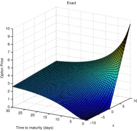
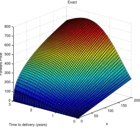
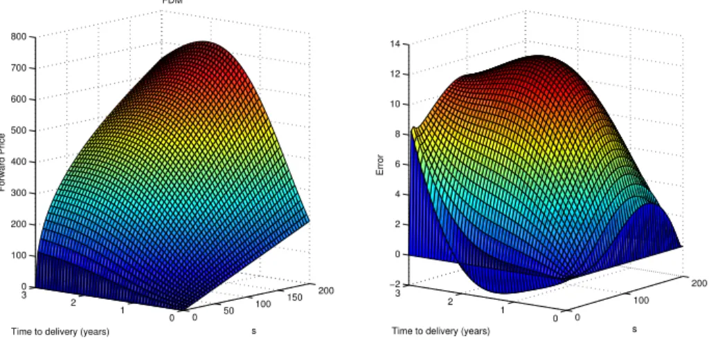
r σ ρ κ η T K

0.03 0.3 0.8 2 0.2 1 100

Figure 2.1 shows the exact solution for the set of parameters given above. The cor-responding finite difference approximation is displayed in figure 2.2. The maximum

absolute error, defined as

MAE(N)=∆ max

0≤i≤I,0≤j≤J|u¯(τN, xi, xj)−U N

i,j|, (2.67)

has been plotted in figure 2.3 as a function of the number of time steps for two distinct sets of spatial bounds. Errors caused by the artificial conditions at Smax and Vmax are lost if the region of interest is sufficiently far from the boundaries.

0 100 200 0 0.2 0.4 0.6 0.8 1 0 20 40 60 80 100 120 s Exact v Option Price

(23)

0 100 200 0 0.2 0.4 0.6 0.8 1 0 20 40 60 80 100 120 s FDM v Option Price 0 100 200 0 0.2 0.4 0.6 0.8 1 −0.07 −0.06 −0.05 −0.04 −0.03 −0.02 −0.01 0 0.01 0.02 0.03 s v Error

Figure 2.2: European call option price in the Heston model computed with Douglas ADI. 0 500 1000 1500 2000 2500 3000 3500 4000 0 0.05 0.1 0.15 0.2 0.25 0.3 0.35

Number of time steps

MAE

Smax = 400 and Vmax = 2 Smax = 800 and Vmax = 4

4.5 5 5.5 6 6.5 7 7.5 8 8.5 −4 −3.5 −3 −2.5 −2 −1.5 −1

Log number of time steps

Log MAE

Smax = 400 and Vmax = 2 Smax = 800 and Vmax = 4

(24)

Chapter 3 American Options

Whereas European options can be exercised only at a single expiration date, Amer-ican style options allow for early exercise at any instant before maturity. The early exercise feature complicates the problem of pricing considerably, and the lack of closed-form solutions has resulted in a rich theory seeking to characterize the option price.

The results in the first part of this chapter are adapted from Myneni [35] and Elliott and Kopp [24].

3.1 General theory

We assume we are working in a complete1_{filtered probability space (Ω}_,_F_,_{F

t}_t≥₀,Q)

satisfying the usual conditions, in the sense that

• F0 contains all the Q-null sets ofF

• Ft=∩u>tFu for all 0≤t <∞, i.e. the filtration is right continuous

The usual conditions will be standing assumptions in all of what follows.

We consider a Black-Scholes market modeled by a bond (or savings account) evolving according to the differential equation

dRt=rRtdt, R0 = 1, (3.1)

and a risky asset, which under an equivalent martingale measure Q is governed by the stochastic differential equation

dSt

St

=rdt+σdWt, S0 =x. (3.2)

(25)

Here, (Wt)t≥0 is a Wiener process on (Ω,F,{Ft}_t≥₀,Q). Let

φ(t) = (φ2(t), φ2(t)),

be a trading strategy in the market, i.e. a set of progressively measurable processes with Z T 0 | φ1(t)|dt+ Z T 0 (φ2(t)S(t))2dt <_∞, a.s. (3.3) whereφ1(t) and φ2(t) denote the holdings at timet in the bond and the risky asset, respectively. We let (Ct)t≥0be a continuous and non-decreasing consumption process with C0 = 0 a.s. Define the corresponding wealth process by

Vt(φ) =φ1(t)Rt+φ2(t)St. (3.4)

The triple (φ1, φ2, C) is said to beadmissible if Vt(φ) is self-financing2, i.e.

Vt(φ) =φ1(0)R0+φ2(0)S0+ Z t 0 φ1(u)dR(u) + Z t 0 φ2(u)dS(u)₋Ct, t∈[0, T], (3.5) and EQ Z T 0 φ2₂(t)S_t2 <_∞. (3.6)

Assumption (3.6) acts as a credit constraint by limiting the amount held in the risky asset. Substituting for the dynamics of the risky asset yields

Vt(φ) =V0(φ) + Z t 0 rVu(φ) + Z t 0 σφ2(u)SudWu −Ct. (3.7)

Recall that a stopping time with respect to our probability space is a random variable

τ(ω) for ω _∈ Ω, such that the event _{τ(ω)_≤t_} belongs to the sigma-algebra _Ft.

Denote by_Tt,T the set of all stopping times with values in [t, T]. In order to straddle

the American put option price, we need the following lemma.

Lemma 3.8. The process

Xt ∆ =ess sup τ∈Tt,T EQ e−r(τ−t)(K₋Sτ)+|Ft , t_∈[0, T], (3.9)

is a wealth process. That is, there exists an an admissible triple (φ1, φ2, C)

corre-sponding to (3.9).

2_{The self-financing condition states that a change in the wealth process results enirely from net} gains or losses.

(26)

Proof. The proof is taken from Myneni [35] and Elliott and Kopp [24]. Let Jt= ess sup τ∈Tt,T EQ e−rτ(K ₋Sτ)+|Ft . t_∈[0, T],

J is theSnell envelope, i.e. the smallest supermartingale dominating the discounted payoff. Moreover, J is c`adl`ag, regular and of class D, thus has the Doob-Meyer decomposition

Jt=Mt−At,

as the difference of a right continuous martingale M, and a unique, predictable continuous and non-decreasing process A, withA0 = 0. From the martingale repre-sentation property under Q(Karatzas and Shreve [30]) we know that there exists a progressively measurable process ψ such that

Z T 0 ψ2udu <∞, a.s. Mt =J0+ Z t 0 ψudWu, ∀t∈[0, T] a.s.

Clearly, Xt =ertJt with dynamics given by

dXt =rertJtdt+ertψtdWt−ertdAt.

Hence, if we put φ1 =Jt−ψtσ−1,φ2(t) =ertψtσ−1St−1 and Ct =

Rt

0 e

rt_dA

t, we have

that Xt=Vt(φ).

Obivously, Xt hedges the American put option in the sense that

Xt≥(K−St)+, t ∈[0, T) a.s.

XT = (K−ST)+, a.s.

The optimal stopping time for the interval [t, T] was charatcerized by El Karoui, and is known to be the first timeJ hits the discounted payoff. That is,

ρt= inf

u_∈[t, T] :Ju =e−ru(K −Su)+ . (3.10)

We are now ready to derive the arbitrage-free price of the option.

Theorem 3.11. If V0 is the initial value of the American put option, then

V0 =X0 (3.12)

(27)

Proof. The proof is taken from Myneni [35] and Elliott and Kopp [24].

Suppose the option trades for the price V0 > X0 at time t = 0, and denote by (β1, β2, c) the trading strategy generating the wealth processXt. Consider the

strat-egy (φ1, φ2, φ3, C) in the bond, stock and the option respectively, augmented by the early exercise policy τ _{∈ T}0,T, given by

φ1(t) = ( β1(t), t_∈[0, τ], β1(τ) +β2(τ)R−1 τ Sτ −R−τ1(K−Sτ)+, t∈(τ, T], φ2(t) = β2(t)1[0,τ](t), φ3(t) = ₋1[0,τ](t), Ct=ct∧τ.

Since Xt hedges the option,

β1(τ)Rτ+β2(τ)Sτ ≥(K −Sτ)+ a.s.,

from which it follows that φ1(T)RT ≥0 a.s. But since

φ1(0) +φ2(0)S0+φ3(0)V0 =X0 −V0 <0, following (φ1, φ2, φ3, C) leads to an arbitrage.

Now, suppose V0 < X0 at time t = 0. With the same trading strategy in X as above, and with exercise policy ρ0 as defined in (3.10),

φ1(t) = ( −β1(t), t_∈[0, ρ0], −β1(ρ0)₋β2(ρ0)R−_ρ₀1Sρ0 +R −1 ρ0(K−Sρ0) +_, _t_∈₍_ρ 0, T], φ2(t) =₋β2(t)1[0,ρ0](t), φ3(t) =1[0,ρ0](t), Ct=−ct∧ρ0,

One can show that the stopped processXt∧ρt is a martingale (see [31] theorem 2.3.1).

Therefore c_≡0 on [0, ρ0] and by definition of ρ0

β1(ρ0)Rρ0 +β2(ρ0)Sρ0 = (K−Sρ0)

+_, _a.s. Henceφ1(T)RT = 0 a.s. and

φ1(0) +φ2(0)S0+φ3(0)V0 =V0−X0 <0. Again there is an arbitrage.

Definition 3.13. Fort ∈[0, T]and x∈R+, define

P(t, x)=∆ sup τ∈Tt,T EQ e−r(τ−t)(K₋Sτ)+|St=x . (3.14)

ThenP(t, x)is the fair price of the American put option, i.e. the price that precludes arbitrage opportunities.

(28)

In as much as (3.10) and (3.14) jointly specify the solution to the option pricing problem, we cannot infer the American option prices explicitly. The characteriza-tion can nonetheless be fruitfully exploited for numerical purposes, which will be our next task.

The optimal stopping problem associated with the option price can be cast as a free-boundary problem, where the domain of the option price is partitioned in two regions according to a free boundary. The free boundary is a time dependent parametriza-tion of the boundary separating opparametriza-tion prices for which it is optimal to exercise immediately, and those for which it is optimal to wait. The free boundary is not known a priori, but rather a part of the solution. Notice that the early exercise feature ensures that P(t, St)<(K−St)+ cannot prevail, otherwise there would be

an arbitrage3_{. Obviously,}

P(t, St)≥(K−St)+, ∀(t, St)∈[0, T)×R+.

P(T, ST) = (K−ST)+.

Thus, we can partition the domain of the option price into the continuation region

C =(t, x)_∈[0, T)_×R+ : P(t, x)>(K₋x)+ ,

and the stopping region

S =(t, x)∈[0, T)×R+ : P(t, x) = (K₋x)+ ,

We need the following properties of the option price (see Jaillet, Lamberton and Lapeyre [27]).

Proposition 3.15. The American put option price P is continuous on[0, T]_×R+,

P(_·, t) is convex and non-increasing on R+ for every t _∈ [0, T] and P(x,_·) is non-increasing on [0, T] for everyx_∈R+_.

The continuity and monotonicity suggest thatP will touch the immediate payoff for some 0< S∗

t < K, 0≤t < T. The time-dependent contact point St∗ for which

P(t, St)>(K−St)+, St> St∗,

P(t, St) = (K−St)+, St≤St∗,

(3.16)

is coined the free boundary, and convexity ensures that this point is indeed unique for eacht _≥0. We see that the optimal stopping time will be the first time instant the asset price hits the free boundary. The economical interpretation of the free boundary goes as follows: suppose 0 ≤ t < T. For St > St∗ immediate exercise

yields the loss (K₋St)+−P(t, St)<0, which is certainly not optimal. If St≤St∗,

(29)

0 5 10 15 20 0 1 2 3 4 5 6 7 8 9 10 S Option price

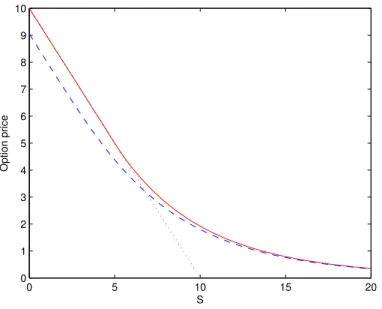
Figure 3.1: Price at t = 0 of an American put option computed by the Brennan-Schwartz algorithm, with K = 10, r = 0.1, σ = 0.6 and T = 1. Dashed line mark the corresponding European option. Dotted line mark the payoff function.

then P(t, St) = K−St and a subsequent change in the underlying asset will cause

a corresponding offset change in the option price. Waiting will only diminish the potential profit Ker(T−t)₋_K_{, so the option should be exercised as soon as} _S

t hits

S_t∗ and the proceeds K reinvested at the risk-free rate.

As St approaches the free-boundary, we must have that that

lim

x→S∗

t

∂P(t, x)

∂x =−1 a.s.

A proof can be found in Myneni [35]. A heuristic argument is that we cannot have

∂P(t,x)

∂x < −1, in which case (3.16) would be violated, and

∂P(t,x)

∂x > −1 implies an

arbitrage. Moreover,P is continuously differentiable over the free boundary, which is known as the principle of smooth fit or smooth pasting.

Now, consider the Black-Scholes option pricing PDE

∂P ∂t + 1 2σ 2_x2∂2P ∂x2 +rx ∂P ∂x −rP = 0, t ∈[0, T). (3.17)

For St ≤St∗, we can deduce that

P(t, St) =K−St, ∂P(t, St) ∂t = 0, ∂P(t, St) ∂x =−1, ∂2P(t, St) ∂x2 = 0. Inserted into the Black-Scholes equation this amounts to

∂P ∂t + 1 2σ 2_x2∂2P ∂x2 +rx ∂P ∂x −rP <0, t∈[0, T), x≤S ∗ t. (3.18)

(30)

On the continuation region the American put price obeys the Black-scholes PDE (??), hence ∂P ∂t + 1 2σ 2_x2∂2P ∂x2 +rx ∂P ∂x −rP ≤0, t∈[0, T), x∈R +_. _(3.19)

We are now ready to state a theorem which provides the basis for a numerical method due to Brennan and Schwarz [13]. See Jaillet, Lamberton and Lapeyre. [27] for a detailed proof of the theorem and a rigorous treatment in favor of the Brennan Schwartz algorithm.

Theorem 3.20. Denote by (St,x

v )t≤v≤T the unique solution to

Sv =b(v, Sv)dv+σ(v, Sv)dWv, v ∈[0, T], (3.21)

starting from x at time t, with corresponding infinitesimal generator

L= 1 2σ(t, x) ∂2 ∂x2 +b(t, x) ∂ ∂x. (3.22)

Let f denote the payoff function for the put option. Assume u is a regular solution of the following system of partial differential inequalities:

     ∂u ∂t +Lu−ru ≤0, t∈[0, T), u≥f ∂u ∂t +Lu−ru (f ₋u) = 0, t_∈[0, T) u(T, x) =f(x), x_∈R+_. (3.23) Then u(t, x) =P(t, x) = sup τ∈Tt,T EQ e−r(τ−t)f(S_τt,x). (3.24)

Proof. This proof is adapted from Lamberton and Lapeyre [32]. The Itˆo formula

applied to ˆu(v, x) = e−rvu(v, x) and Svt,x yields

ˆ u(v, S_vt,x) = ˆu(t, x) + Z v t e−rs ∂u ∂v +Lu−ru (s, S_st,x)ds+ Z v t e−rs∂u(s, S t,x s ) ∂x σ(s, S t,x s )dWs. So Mv = ˆu(v, Svt,x)− Z v t e−rs _∂u ∂v +Lu−ru (s, Sst,x))ds

is a Q-martingale. The Optional sampling theorem applied to this martingale with the stopping timest and τ givesEQ[Mτ] =EQ[Mt]. As ∂u_∂v +Lu−ru ≤0, we have

that

u(t, x)≥EQ

(31)

Furthermore, using that u_≥f, u(t, x)_≥EQ e−r(τ−t)f(S_τt,x). Hence u(t, x)_≥ sup τ∈Tt,T EQ e−r(τ−t)f(S_τt,x)=P(t, x).

Let τ∗ = inf_{t_≤s_≤T :u(s, S_st,x) =f(S_st,x)_}, and observe that τ∗ is a _{Ft}_t≥₀

stopping time. We know that for s_∈ [t, τ∗₎

∂u

∂v +Lu−ru

(s, Sst,x) = 0.

In this case, the Optional sampling theorem yields

u(t, x) =EQ e−r(τ∗−t)u(τ∗, S_τt,x∗) =EQ e−r(τ∗−t)f(S_τt,x∗) .

Moreover,u(t, x)_≤P(t, x), so u(t, x) =P(t, x) andτ∗ is the optimal stopping time.

3.2 The Brennan-Schwartz Algorithm

Brennan and Schwartz [13] proposed a simple and efficient algorithm to solve the system of inequalities (3.23) by finite differences. They applied an implicit scheme and proceeded as in the European case, but with a modification in the tridiagonal matrix algorithm accounting for early exercise. To ease notation, we assume time-independent coefficients, i.e

b(t, x)≡b(x) and σ(t, x)≡σ(x).

Assume the spatial domain has been localized to (0, Smax) with homogeneous Dirich-let boundary conditions. The computational grid is given by

{(tn, si) : n = 0, ..., N, i= 0, ..., I}.

The discretized system of inequalities can be written as

     LUn+1 _≤_b Un_≥_f (LUn+1₋_b₎T₍_Un₋_f_{) = 0} (3.25) where L=I+θ∆tA is a (I₋1)×(I₋1) matrix, Un₌ _Un 1, ..., UI−n 1 T ∈RI−1 (3.26) f = (f(s1), ..., f(sI−1))T ∈RI−1 (3.27) b= (I−(1−θ)∆tA)Un∈RI−1 (3.28)

(32)

and A=          β1 γ1 0 α2 β2 γ2 . .. ... . ..

αI−2 βI−2 γI−2

0 αI−1 βI−1          ,          αi = 1₂ _σ2 i ∆x2 − bi ∆x βi = 1₂ _σ2 i ∆x2 −r γi = 1₂ _σ2 i ∆x2 + bi ∆x .

We solve the system (3.25) by the modified tridiagonal matrix algorithm:

γ_i0 = (_γ i βi, i= 1 γi βi−γi0−1αi, i= 2, ..., I−2 b0i = (_b_i βi, i= 1 bi−b0i−1αi βi−γi0−1αi, i= 2, ..., I−1 (

U_I−n+1₁ = maxb0_I−₁, f(sI−1)

U_in+1 = maxb0i−γi0Ui0+1, f(si) , i=I−2, ...,1

Time-homogeneous boundary conditions can be chosen according to

• Dirichlet type: u(tn, x0) =g0,u(tn, xI) =gI

• Neumann type: ∂u(tn,x0)

∂x =g0,

∂u(tn,xI)

∂x =gI

for n = 0, ..., N₋1. Non-homogeneous Dirichlet boundaries are realized in the the vector b as b= (I₋(1₋θ)∆tA)Un₊        −α1g0 0 .. . −γI−1gI        ,

whereas non-homogeneous Neumann boundaries4 _{alter the matrix} _A_to

A=          β1+α1 γ1 0 α2 β2 γ2 . .. ... . ..

αI−2 βI−2 γI−2

0 αI−1 βI−1 +γI−1

         .

(33)

In chapter 5 we apply an extension of this algorithm in conjunction with the Dou-glas ADI scheme. The idea is taken from Villeneuve and Zanette [43] and Villeneuve and Zanette [44] where the Douglas-Rachford ADI scheme is applied to American two-factor options. The method is referred to as LCP-ADI (linear complementar-ity problem ADI), and essentially involves an application of the Brennan-Schwartz algorithm in each direction of the ADI scheme.

3.3 The Longstaff-Schwartz Algorithm

We have formulated the American option price in terms of an optimal stopping prob-lem and a set of partial differential inequalities. The system of inequalities can be solved by finite difference methods such as the Brennan-Schwartz algorithm. How-ever, multiple dimensions are notoriously difficult to handle with finite differences. The algorithm due to Longstaff and Schwartz [33] confines the stopping problem to a discrete optimization problem which can be tackled by Monte Carlo and dynamic programming. By replacing the continuum of exercise dates by a finite subset, we can essentially approximate the American option by a so-called Bermudan option. The algorithm involves simulating asset paths and replacing conditional expecta-tions by projecexpecta-tions onto a finite set of basis funcexpecta-tions. Since we are restricting the set of stopping times to a smaller subset, the approximation is expected to produce a sub-optimal early exercise strategy, effectively yielding a low-biased estimate for the option value. Analogously, if the exercise strategy is based on information an-ticipating the future, we obtain a high-biased estimator. In combination, simulation of low- and high-biased estimators can be used to construct a confidence interval for the option. A detailed account on American options and simulation techniques is given in Glasserman [25]. Here we discuss the algorithm as presented in the original paper by Longstaff and Schwartz.

Let T denote the maturity of the option. We divide the time to maturity into N

equidistant intervals of length ∆t, such that 0 = t0 < t1 < ... < tN = T, and

generate independent sample paths nS_i(j)o

N

i=1, j = 1, ...M, whereM is the number of Monte Carlo simulations. LetI_i(j) denote the intrinsic value of the option at time

ti for the jth asset path, i.e. the payoff from immediate exercise. Similarly, let C( j)

i

denote the continuation value from not exercising the option at time ti. Dynamic

programming yields the following backward recursion for the American put option:

   V_N(j) =I_N(j)=K ₋S_N(j)+ V_i(j) = maxnI_i(j), C_i(j)o, i=N ₋1, ...,0, (3.29) where C_i(j)=EQ h e−r∆tV_i(₊₁j) _| S_i(j)i. (3.30)

(34)

In order to keep track of the early exercise strategies we introduce some additional notation. Let_Ti,N denote the possible stopping times at timeti taking values in the

finite set _{i, ..., N_}. The stopping times are defined as

τ_i(j)= min∆ nk _≥i _|V_k(j) =I_k(j)o, (3.31) which can be used to reformulate the continuation value. Let

C_i(j)=EQ h e−r∆t(τi(+1j)−i)I(j) τi+1 | S (j) i i . (3.32)

This expression will be the key quantity in the regression.

To reduce computational efforts, Longstaff and Schwartz proposed to use only in-the-money sample paths. Accommodating for ”moneyness”, dynamic programming in terms of stopping times amounts to

       τ_N(j) =N τ_i(j) =i1n I_i(j)≥C_i(j)o∩nI_i(j)>0o +τi+11n I_i(j)<C(_ij)o∪nI_i(j)=0o, i=N −1, ...,0. (3.33)

Note that the exercise strategy cannot be deduced along individual paths separately, as this would exploit knowledge of the future and imply clairvoyance. Instead, in each time step we use the simulated asset paths to obtain an estimate of the continuation value. The conditional expectation in (3.32) is an element in L2, and we can readily justify representing Ci(j) as a linear combination of basis functions

from a countable Fti-measurable set. Thus, in each time stepi prior to maturity we

must solve the regression problem

e−r∆t(τi(+1j)−i)I(j) τi+1 = K X k=1 βk,iψk(S( j) i ) +j, j = 1, ..., M, (3.34)

for a suitable choice of basis functions ψi(j) =

ψ1(Si(j)), ..., ψK(S( j) i ) T . A simple least-squares procedure yields

ˆ βi = arg min βi∈RK 1n I_τi(j₊₁) >0o M X j=1 e−r∆t(τi(+1j)−i)I(j) τi+1−βi·ψ (j) i 2 . (3.35)

Put ˆC_i(j) = ˆβi ·ψi(j). The algorithm proceeds by replacing the continuation value

by its least-squares estimate, and deducing the exercise decision from the recursion (3.33). We obtain an exercise strategy ˆτ(j)_{, j} _{= 1}_{, ..., M}_{, for each sample path. The} Least-Square Monte Carlo (LSM) option price will be given by

ˆ V0 = max ( I0, 1 M M X j=1 e−r∆tτˆ(j)I_ˆ_τ(j(j)) ) , (3.36)

(35)

where I0 = (K −S0)+ is the immediate payoff at timet = 0 and S0 is the (deter-ministic) initial asset price.

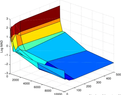
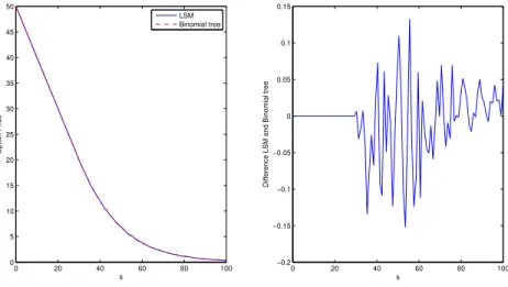
According to Longstaff and Schwartz [33] the algorithm is fairly robust to the choice of basis functions. They also indicate, through numerical testing, that a modest number of basis functions provide satisfactory results. Even the simple set of mono-mials ψ1(x) = 1, ψ2(x) =x, ψ3(x) =x2 is performing well5. Orthogonal polynomi-als, including the Hermite, Laguerre and Legendre are also common. A numerical convergence study for the Black-Scholes model is provided in 3.2. We employ the simple monomials and use Matlab’s built-in binomial tree algorithm as our refer-ence. Convergence is measured in the maximum absolute difference (MAD), and one may verify the (infamous) square-root convergence of Monte Carlo. Solutions in both algorithms are given in figure 3.3 (lines overlap).

0 2000 4000 6000 8000 10000 0 100 200 300 400 500 −3 −2 −1 0 1 2 3

Number of time steps N Number of Monte Carlo simulations

Log MAD

Figure 3.2: Convergence of the Longstaff-Schwartz algorithm for the Black-Scholes model.

(36)

0 20 40 60 80 100 0 5 10 15 20 25 30 35 40 45 50 Option Price s LSM Binomial tree 0 20 40 60 80 100 −0.2 −0.15 −0.1 −0.05 0 0.05 0.1 0.15

Difference LSM and Binomial tree

s

Figure 3.3: Price of an American put option computed by the Longstaff-Schwartz algorithm and Matlab’s binomial tree algorithm.

(37)

Chapter 4 Carma Processes

The parametric class of continuous-time autoregressive moving average processes is the natural extension of the discrete ARMA models from time series analysis. CARMA provides a convenient modeling framework accounting for memory effects and mean-reversion, with the the decisive benefit of stochastic calculus over discrete-time models. Early works on CARMA processes go all the way back to the 1950s. A renewed interest in these models stems from the prevailing interest in financial econometrics, and in particular in Ornstein-Uhlenbeck processes (OU) such as the acclaimed stochastic volatility model proposed by Barndorff-Nielsen and Shepard [3]. CARMA can be seen as a higher-order generalization of the stationary OU pro-cess, and can easily reproduce a variety of temporal dependence structures. They effectively provide a flexible alternative to modeling by linear combinations of in-dependent OU processes. CARMA models have also been successfully applied to irregularly-sampled data, as is frequently encountered in finance or in the case of data with missing observations. An introduction to CARMA processes is given in Brockwell [15] and Brockwell [14]. Recent applications of CARMA models include interest rate modeling, electricity markets, weather markets and stochastic volatility. We review L´evy-driven CARMA processes and indicate how they extend the famil-iar OU process. OU is a special case of the continuous time autoregressive (CAR) processes, and will also be referred to as CAR(1).

4.1 L´

evy-driven CARMA processes

Definition 4.1. A L´evy-driven CARMA(p,q) process (Yt)_t≥₀ (with 0 ≤ q < p) is

defined as the solution of the state-space equations

Yt=bTXt (4.2)

(38)

with A =          0 1 0 · · · 0 0 0 1 · · · 0 ... ... . .. ... 0 0 0 _{· · ·} 1 −αp −αp−1 −αp−2 · · · −α1          , ep=          0 0 ... 0 1          , b =          1 b1 ... bp−2 bp−1          , Xt=           Xt X_t(1) ... Xt(p−2) Xt(p−1)           .

where(Lt)_t≥₀ is a L´evy process andα1, ..., αp>0andb1, ..., bp−1 are complex-valued

coefficients such that bj = 0 for q < j ≤ p. For p = 1, the matrix A is to be

understood as A=−α1.

In the case bj = 0, j ≥1, the Y becomes a CAR(p) process.

The CARMA process can be represented as the suitably interpreted1 _strictly sta-tionary solution to the pth order linear SDE

a(D)Yt =b(D)DLt, t≥0, (4.4)

in which D denotes differentiation with respect to time, and

a(z)=∆ zp +α1zp−1 +...+αp

b(z)= 1 +∆ b1z+...+bp−1zp−1

(4.5) are the characteristic polynomials of Y. Here, stationarity is assumed in the sense that all finite dimensional distributions are shift-invariant. To this end, we make the following standing assumptions to ensure strict stationarity:

• The characteristic polynomials have no common zeros.

• Eln_|L1|+<∞.

• All eigenvaluesλ1, ..., λpofA are distinct and have strictly negative real parts,

i.e. _Re(λj)<0, j = 1, ..., p.

A proof can be found in Brockwell and Lindner [17]. These assumptions also make sure that Xis a causal process, makingY causal as well. It is easy to check that the eigenvalues of the matrixAcorrespond to the zeros of the autoregressive polynomial

1_DL

(39)

a(z).

The following lemma can be proved by an application of the multi-dimensional Itˆo formula for semimartingales (Protter [38]).

Lemma 4.6. The solution of (4.3) starting at times_≥0is given by the stochastic

process Xt=e A₍_t−s₎ Xs+ Z t s eA(t−u)epdLu, t≥s, (4.7)

where, for any square matrix A, the matrix exponential is defined as

eA ∆ =I+X k≥1 1 k!A k_. _(4.8)

Note that the integral is interpreted as integration with respect to a semimartingale. Given Xs, we can now expressY as

Yt=bTe A₍_t−s₎ Xs+ Z t s bT_eA₍_t−u₎ epdLu, t ≥s. (4.9)

By the independent increment property of L´evy processes, XandY are readily seen to be Markov processes. The Markov property is the key to the derivation of the pricing PDEs in chapter 5.

The CARMA process is often given in terms of its kernel,2 _g₍_t_{) =}_bT_eA_t

ep1[0,∞)(t), and we may write

Yt=

Z t −∞

g(t₋u)dLu.

The kernel determines the memory of the CARMA process, and gives the weights with which the past observations enter the integral (??). Since A is a companion

matrix with distinct eigenvalues, it is diagonalizable as

A=VΛV−1, (4.10)

whereΛ= diag{λ1, ..., λp} andV is theVandermonde matrix corresponding to the

λ’s. It follows that the right eigenvectors corresponding to the matrix A are

1, λj, λ2j, ..., λ p−1 j , j = 1, ..., p.

2_{This formulation requires an extension of} _L _{to a process defined on the index set (}_−∞_,_∞_). This is done by introducing an independent copy,L˜t

t≥0, and defining

L∗_t =Lt1[0,∞)(t)−L˜−t−1(−∞,0](t), ∞< t <∞. Then relabel L∗ _as_L_.

(40)

Brockwell and Lindner [17] assert that bT_eA_t ep = 1 2πi Z γ b(z) a(z)e tz_dz, _(4.11)

whereγ is a simple closed curve enclosing all eigenvalues of A. We may deduce that (see the appendix)

g(t) = p X j=1 eλjt b(λj) a(1)₍_λ j) , t _≥0, (4.12)

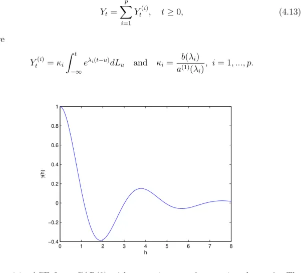
where a(1) denotes differentiation of a(_·). This representation of the kernel provides a decomposition ofY into a sum of dependent and possibly complex-valued CAR(1) processes, Yt = p X i=1 Yt(i), t ≥0, (4.13) where Y_t(i) =κi Z t −∞ eλi(t−u)_dL u and κi = b(λi) a(1)₍_λ i) , i= 1, ..., p. 0 1 2 3 4 5 6 7 8 −0.4 −0.2 0 0.2 0.4 0.6 0.8 1 h γ (h)

Figure 4.1: ACF for a CAR(2) with α1 = 1, α2 = 3, σ = 1 and t = 0. The autoregressive coefficients yield complex eigenvalues.

Furthermore, if E[L2

1]<∞, the autocovariance function is given by

γ(h) = Cov [Yt+h, Yt] =σ2 p X j=1 b(λj)b(−λj) a(1)₍_λ j)a(−λj) eλj|h|_, _(4.14)

(41)

where σ2 = Var [L1]. For a CAR(1) process, b(z) = 1 and a(z) = z +α, which amounts to γ(h) = σ 2 2αe −α|h|_.

Under the assumptions of stationarity and square-integrability the autocorrelation function (ACF) is given by

ρ(h) = Corr [Yt+h, Yt] =

γ(h)

γ(0). (4.15)

We see that the ACF of a CAR(1) process is constrained by monotonicity, whereas CARMA allows for a more complex ACF without introducing additional factors. Figure 4.1 shows the ACF of a CARMA process with damped oscillatory autocorre-lation. Observe that the CARMA process is driven by a single source of randomness, although the state vector is p-dimensional. From the eigen-decomposition (4.10) we have that eA_t

= VeΛt_V−1_{, so the components of the vector} _eA_t

Xs are linear

com-binations of the eigenvalues, and each component will exhibit different speed of mean-reversion3. Moreover, withq _≥ 1 we are able to mimic the effect of multiple CAR(1) factors while retaining the advantage of working with a single distribution. In this respect, CARMA(2,1) is a parsimonious, yet flexible model for a variety of applications.

4.2 Gaussian CARMA processes

We end this chapter by considering the class of Gaussian CARMA models suitable for wind-speed and temperature modeling. The observation and state equations take the form

Yt=bTXt, (4.16)

dXt =AX_tdt+e_pσ(t)dW_t, t ≥0, (4.17)

where (Wt)_t≥₀ is a Wiener process and σ(t) is a continuous, real valued function

bounded away from zero. In weather modeling σ(t) is observed to be a periodic function. Benth [5] shows that Y remains stationary when volatility is bounded. A straightforward application of the multi-dimensional Itˆo formula verifies that the solution of (4.17), starting at times, is the multi-dimensional Gaussian OU process

Xt=e A₍_t−s₎ Xs+ Z t s eA(t−u)epσ(u)dWu, t≥ s. (4.18)

By well-known properties of the Itˆo integral,

E[Yt | Xs] =bTe A₍_t−s₎ Xs, (4.19) Var [Yt | Xs] = Z t s bTeA₍_t−u₎ ep 2 σ2(u)du. (4.20)

(42)

It can be verified that the limiting distribution ofY exists under the above assump-tions and is Gaussian with mean zero and variance

lim t→∞ Z t 0 bT_eA₍_t−u₎ ep 2 σ2(u)du.

(43)

Chapter 5 Modeling and Pricing in

Electricity and Weather Markets

In this chapter we present spot electricity and temperature models and discuss the implications of non-storability on pricing. We derive pricing PIDEs and PDEs which we attempt to solve with numerical methods discussed in the preceding chapters.

5.1 Electricity Derivatives

Over the last decades there has been a vast deregulation of electricity markets, start-ing in the late 1980s when the UK initiated a privatization and restructurstart-ing of the electricity sector. By now, the European market is fully liberalized, and both phys-ical and purely financial contracts are available for producers, retailers, consumers and speculators. The rich interplay between regulation, production and distribution renders electricity markets highly complex, and a variety of contracts are traded in order to control risk and secure efficient operation of the physical network.

Forward prices can be modeled by a direct specification of the forward dynamics or be derived in terms of the spot. The lack of storability makes the spot-forward con-nection questionable, and the Heath-Jarrow-Morton framework from fixed-income markets is often adopted for a direct approach. Spot price modeling is nonetheless interesting per se, and we consider a two-factor jump-diffusion model in which we eventually derive forward prices numerically and in closed-form. The general setup is taken from Benth et al. [6], and the CAR(1) process will be our main modeling tool.

Let (St)_t≥₀ be a stochastic process modeling the spot electricity price defined on the

complete filtered probability space Ω,_F,_{F}_t≥₀,Psatisfying the usual conditions. Our first step is to decide on either of the following basic classes of models:

(44)

Arithmetic Model St = Λ(t) + m X i=1 X_ti+ n X j=1 Ytj, X₀i +Y₀j =S0−Λ(0), i= 1, ..., m, j = 1, ..., n (5.1) Geometric Model lnSt= ln Λ(t) + m X i=1 X_ti+ n X j=1 Y_tj, X₀i +Y₀j = lnS0−ln Λ(0), i= 1, ..., m, j = 1, ..., n (5.2)

Here, Λ is a deterministic seasonality function,

dX_ti = (µi(t)−αi(t)Xti)dt+ p X k=1 σik(t)dWtk, i= 1, ..., m, (5.3) and dYtj = (δj(t)−βj(t)Ytj)dt+ηj(t)dLjt, j = 1, ...n. (5.4) Wk t

t≥0are independent Wiener processes and (Lt)t≥0is a L´evy process independent of Wk

t for all t ≥ 0 and k = 1, ..., p. This setup subsumes many spot price models

advocated in the literature, and can be employed to account for the stylized features observed in the market, such as

• Seasonality (yearly, monthly, weekly and daily)

• Mean reversion

• Price spikes

• Time dependent volatility

Note that since L´evy processes have independent and stationary increments, this framework does not capture the time dependency in jump size and jump intensity observed in the market1_{. The class of} _{independent increment} _{(II) processes treated} in Benth et al. [6] provide the necessary degree of generality.

The most common models for commodity and equity prices are of geometric type, i.e. having an exponential structure. Geometric models ensure non-negativity of prices2_{, making them a natural choice for modeling purposes. However, in energy} markets such as electricity and gas, our main interest is pricing contracts delivering the spot over some prescribed period of time, so-calledswapcontracts, and contracts

1_{In the Nordic markets large price spikes are more frequent during winter.}

2_{Negative prices are occasionally observed in electricity and gas markets. In electricity markets} this is due to an excess of power in the grid, in which case paying someone to consume the electricity is cheaper that shutting down generators.

(45)

derived from the swaps. Geometric models often yield complicated expressions for the these contracts, whereas the additive structure of arithmetic models allows con-siderably more tractability. Moreover, negative prices can be circumvented by using a subordinator (or more generally, an increasing II process) in the driving noise, so there is no reason to confine the spot models to those of geometric type.

A Jump-Diffusion Spot Model

We give a brief excursion to L´evy processes intended to introduce notation and terminology. Let L = (Lt)_t≥₀ be a stochastic process defined on our probability

space.

Definition 5.5. An adapted process L with L0 = 0a.s. is a L´evy process if

• L has independent increments, i.e. Lt−Ls is independent of Fs for 0 ≤s <

t <_∞

• Lhas stationary increments, i.e. Lt−Ls has the same distribution as Lt−s for

0_≤s < t <_∞

• L is continuous in probability, i.e. for all s_≥0 lim

t→sP (|Lt−Ls| ≥) = 0, ∀ >0

Every Lévy process has a unique càdlàg3 _{modification, and we therefore assume that}

L is indeed already c`adl`ag. Define thejump of L at time t_≥0 as ∆Lt

∆

=Lt−Lt−, where Lt−= lim

s↑t Ls. (5.6)

Associated with L is a Poisson random measure N = (N(t, A), t_≥0, A_∈R0) de-fined as

N(t, A)=∆ X

s≤t

1∆Ls∈A, (5.7)

where A is a Borel subset in R0 = R\ {0}. N counts the number of jumps falling in the set A occuring before or at time t, and since L is càdlàg there can only be a finite number of jumps bounded from below (i.e. N(t, A) < _∞ if 0 _6∈ A). The corresponding Lévy measure is defined as

ν(A)=∆ E[N(1, A)], A _{∈ B}(R0), (5.8) which is a σ-finite measure on _B(R0), satisfying

Z

R0

(_|z_|2_∧1)ν(dz)<_∞. (5.9)

Numerical Option Pricing in CARMA Models