Economico-Finanziarie XXVI ciclo
Efficient tree methods
for option pricing
Thesis submitted in partial fulfillment of the requirements for the degree of
Doctor of Philosophy in
Mathematics for Economic-Financial Applications
by
Elisa Appolloni
Program Coordinator
Thesis Advisors
Prof. Dr. Maria B. Chiarolla
Prof. Dr. Lucia Caramellino
Introduction 1
Double and multi-step double barrier options . . . 3
Barrier options on discontinuous payoff functions . . . 7
Options on a model with CIR interest rate . . . 9
1 Mathematical background 15 1.1 Convergence of Markov chains to diffusions . . . 15
1.1.1 Weak convergence result . . . 16
1.1.2 Weak convergence of the CRR binomial tree . . . 20
1.1.3 Nelson and Ramaswamy technique for diffusion approximations . . . 22
1.1.4 Convergence of the American prices . . . 27
1.2 The rate of convergence of European options in the CRR tree . . . 30
1.2.1 Rate of convergence for vanilla options . . . 30
1.2.2 Rate of convergence for barrier options . . . 36
2 Double and multi-step double barrier options in the Black and Scholes model 45 2.1 The model . . . 48
2.2 The closed-form formulas . . . 49
2.3 Lattice procedures for barrier options . . . 52
2.4 The Dai and Lyuu procedure . . . 53
2.5 The binomial interpolated lattice . . . 55
2.6 Rate of convergence in the European case . . . 58
2.7 The binomial interpolated lattice for step double barrier options . . . 64
2.8 Numerical results . . . 67
2.8.1 Double barrier options: comparisons with the Day-Lyuu method . . . 67
2.8.2 Double barrier options: comparisons with a finite difference method . 69 2.8.3 2-step double barrier options . . . 71
2.8.4 Multi step double barrier options . . . 72
3 Digital barrier options in the Black and Scholes model 75 3.1 Digital call options with single barrier . . . 76
3.1.3 Binomial error for digital call options with a single barrier . . . 84
3.2 Double barrier options on discontinuous payoffs . . . 92
3.2.1 Preliminary results . . . 94
3.2.2 Upper bound for the error . . . 96
3.3 Numerical results . . . 101
3.3.1 Single barrier digital options . . . 101
3.3.2 Double barrier digital options . . . 107
4 Option pricing with CIR interest rate 115 4.1 Pricing American options on two state variables or with stochastic interest rate117 4.2 The bivariate continuous model . . . 119
4.3 Existing lattice methods in the BS-CIR model . . . 120
4.3.1 The Wei procedure . . . 120
4.3.2 The Hilliard,Schwartz and Tucker procedure . . . 124
4.4 The new bivariate algorithm . . . 125
4.5 The convergence . . . 128
4.5.1 Weak convergence of the associated approximating Markov chain . . 128
4.5.2 The convergence of the prices . . . 139
4.6 Numerical results . . . 143
A Proof of Lemma 3.2.4 and Lemma 3.2.5 149 A.1 Proof of Lemma 3.2.4 . . . 149
A.2 Proof of Lemma 3.2.5 . . . 154
The aim of this dissertation is the study of efficient algorithms based on lattice procedures for dealing with two relevant issues arising in the recent literature on option pricing: the pricing of complex barrier-type options and the pricing of options when the equity model takes into account a stochastic interest rate. This research is developed with a twofold perspective: first, we propose a good solution from a numerical point of view through the introduction of efficient lattice procedures and secondly, we study the theoretical aspects related to the tackled problems. Tree-based algorithms for option pricing are studied since the seminal work of Cox, Ross and Rubinstein ([28], 1979) and turn out to be very simple and fast to be implemented by a backward induction. An important characteristic which makes these procedures very appealing is that they easily include American-style features once the European case is treated and well set up. This makes lattice techniques widely used in the practice because although many progresses have been done in the development of exact formulas or other numerical procedures (Monte Carlo, finite differences, etc.) for European option prices, the American counterparts, that involve a control problem, are not so well-provided.
The mathematical background underlying the approximation of diffusion processes with tree methods is briefly developed in Chapter 1. Roughly speaking, we can recall such methods as follows. Let X denote a diffusion process, that is the solution to the following stochastic differential equation (SDE):
dXt=b(Xt)dt+σ(Xt)dBt, X0 =x0. (0.0.1)
For the sake of simplicity, we assume to be in the 1-dimensional case, so the drift coefficient
b and the diffusion coefficient σ denote suitable functions and B stands for a standard Brownian motion in R. A tree-method consists in approximating the evolution ofX over a time interval [0, T] by means of a suitable Markov chain: one fixes 0 =t0 < t1 <· · ·< tn=T
with tk = kh = kT /n, k = 1, . . . , n, and construct a Markov chain (Xkh)k=0,...,n such that,
as h → 0, for every k then Xh
k is “close to” Xtk. More precisely, by setting ¯X
h as the
continuous-time process given by the linear interpolation in time of the Markov chain Xh,
that is ¯ Xth = (k+ 1)h−t h X h k + t−kh h X h (k+1)h, kh≤t <(k+ 1)h, (0.0.2)
then the Markov chains Xh are set in order that ( ¯Xh)h converges in law on the space of
about the Markov chain? It is built possibly in a “simple way”, that is as a Markov process (in discrete time and space) running on a computationally simple lattice. We deal here with a binomial lattice: at each time-step k, the Markov process may do only two jumps, an up-jump or a down-jump, and the jump-probabilities are set in order to achieve the convergence, see Section 1.1.3. This means that the approximating process evolves on a very simple structure, see Figure 1.
Figure 1: Binomial tree with 3 time steps.
We consider here the Black and Scholes model, which is either classical and still widely used in finance. This means that the underlying asset price process (St)t∈[0,T]evolves as the
diffusion process (0.0.1) in which b and σ are chosen linear and non-affine that is
dSt =rStdt+σStdBt, S0 =s0 >0, (0.0.3)
wherer is the interest rate andσ is the volatility parameter. For more details one can refer to Black and Scholes ([13], 1973) and Merton ([64], 1973). Notice that (0.0.3) says that we are writing the dynamics under the risk-neutral measure. We recall that (0.0.3) means that (St)t∈[0,T] evolves as a geometric Brownian motion and, roughly speaking, in a small time
interval ∆t, the percentage variation ∆St
St is approximately a Gaussian r.v. with mean r∆t
and variance σ2∆t.
Option prices with the underlying stock price process following the SDE (0.0.3) can be computed by using the simple tree method due to Cox, Ross and Rubinstein ([28], 1979), CRR in what follows. We briefly recall the procedure in [28]. We define h =T /nand then
we build a binomial tree with n time-steps of length h. We label (0,0) the starting node that corresponds to the value S0 =s0. At time stepih, the discrete process may be located
at one of the nodes (i, j) corresponding to the values
Si,j =s0e(2j−i)σ
√
h, i= 0,1, ..., n, j = 0,1, ..., i. (0.0.4)
Hence, starting from Si,j at time ih, the process may jump at time (i+ 1)h to the value Si+1,j+1 or to the value Si+1,j with probability pand 1−p respectively, wherepis defined as
p= e
rh−d
u−d , (0.0.5)
where u=eσ
√
h =d−1. We remark again that the advantage of this procedure is that both
European and American prices can be easily calculated.
However financial derivatives have been becoming more and more sophisticated and this means that the standard implementation of the CRR binomial tree brings to further errors in the approximation of the Black and Scholes prices. This is the reason why it becomes important to set up “efficient tree schemes”, that are tree methods which allow one to reduce the approximation errors.
In what follows, we briefly present the innovative contribution given in this thesis with respect to the existing literature on some complex option pricing topics, without leaving out the reasons for which they are intensively used in practice. More precisely, we deal with the following arguments:
1. double and multi-step double barrier options; 2. barrier options on discontinuous payoff functions. Then, we build and study a more complex efficient tree for:
3. options in a model where the interest rate is no more constant and deterministic and follows the Cox, Ingersoll and Ross process ([27], 1985), CIR hereafter.
We now describe in details the content of this dissertation by means of three paragraphs that correspond to the three main chapters of this thesis.
1. Double and multi-step double barrier options
Barrier options are path-dependent options that become activated or nullified if the under-lying asset price reaches certain levels. Double barrier options are characterized by two price levels that are located above (higher barrier) and below (lower barrier) the initial stock price. If we denote with f a generic payoff function, then the payoff of a double barrier knock-out option with payoff f is given by:
f(ST)1Sinf>L,Ssup<H, Sinf = inf
where L and H denote the lower barrier and the higher barrier respectively. In particular we consider call and put options, i.e. f(x) = max(θ(x−K),0) with θ = 1 for call options and θ =−1 for put options, K standing for the strike price.
Nowadays barrier options are frequently traded because they have some features that make them more attractive than standard or vanilla options. In fact they are less expensive than vanilla contracts because they can be knocked-out or knocked-in. Moreover, they are much more flexible than standard contracts because they allow to set knock-out or knock-in levels depending on the expectations and the needs of the customers. For example they are widely used in the foreign exchange markets. In fact barrier options are embedded in financial products used to allow for hedging strategies in order to protect the holder from a potential appreciation and/or depreciation of the foreign currency with respect to the domestic one. They are also standard ingredients of a variety of structured products of range-type and it is also possible to find a barrier-type structure for example in loans and forward contracts (for details see Wystup ([86], 2006)).
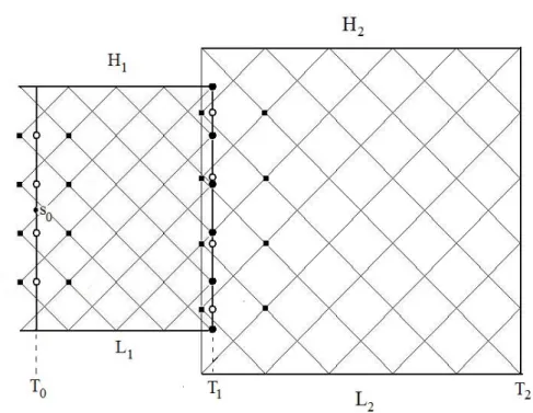
A closed-form formula for pricing European double barrier call and put options when the underlying process follows the SDE (0.0.3) exists when the two barriers are exponential functions of the time (see Kunitomo and Ikeda ([56], 1992)). In the special case in which the barriers are constant, the price can be derived by using techniques involving the Laplace transform of the option price (see Geman and Yor ([40], 1996)). This issue has also been approached by authors such as Kolkiewicz ([55], 1997), Sidenius ([73], 1998) and Pelsser ([67], 2000). Quasi-analytical expressions for American options are presented in Gao and Subrahmanyam ([36], 2000), but we remark that here just a single barrier is considered. Since in all the previous cases it is not possible to price American-style double barrier call and put options, numerical methods have been examined in the literature. It is known that a naive application of the standard CRR binomial tree may lead to a very slow convergence if the barrier is not chosen at a sufficiently small distance with respect to a layer of nodes of the tree (see Boyle and Lau ([16], 1994)). Then a possible solution is to set the algorithm such that the barrier lies exactly on the lattice, as in Ritchken ([72], 1995), Cheuk and Vorst ([22], 1996), Figlewski and Gao ([34], 1999), Gaudenzi and Lepellere ([37], 2006) and Gaudenzi and Zanette ([39], 2009). However, all the previous lattice methods are only able to deal with a single barrier. The first attempt that considers the possibility of efficiently pricing double barrier options with a tree method is due to Dai and Lyuu ([29], 2010). They are able to construct a binomial mesh by choosing the time step such that both the lower barrier and the upper barrier are exactly on two nodes of the tree at maturity (see Section 2.4 for details). However their method is not able to deal with the “near barrier problem”, that consists in a failure of the computational procedure (unless one drastically increases the number of time steps of the algorithm) when the initial asset price is close to one of the barriers.
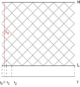
Then we introduce a new algorithm, called the Binomial Interpolated Lattice (BIL hereafter), that is based on the Dai-Lyuu idea of defining the time step ∆t such that the barriers are exactly matched at maturityT with two layer of nodes in the lattice. As explained in Section 2.5, the time step ∆t is obliged to take some specific values in order to match both the lower
barrier Land the higher barrier H and this implies that ∆Tt ∈/ N. In order to arrive close to time 0, we add two further steps of length ∆t and so we get a fictitious time t0 < 0 and a
time t1 >0, see Figure 2.
Figure 2: Binomial interpolated lattice mesh.
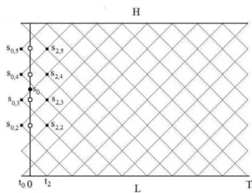
Since we do not know a priori if the initial prices0is a point of the lattice (and in general it is
not), the approximating option price at (0, s0) is provided by suitable interpolations in time
and in space involving the prices which are computed by the standard backward induction at times t0 and t2. We also notice that the prices at t0 < 0 have not a financial meaning,
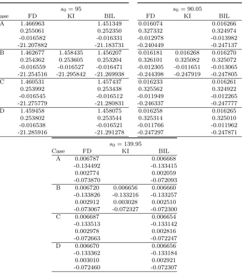
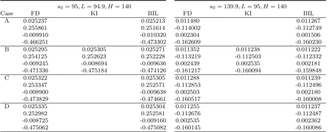
but from the mathematical point of view we are supposing to extend by continuity the price function for negative times and this allows us to set up the computational procedure. The proposed algorithm turns out to be efficient: it gives accurate results for every value of the initial asset price. In particular, numerical experiments show that it provides precise double barrier option prices when compared to the Kunitomo and Ikeda closed-form formula ([56], 1992) and also to the finite difference method of Zvan, Forsyth and Vetzal ([87], 2000). We also remark that the values of the delta, vega and gamma computed by using a finite difference approximation on the prices given by the lattice turn out to be comparable with the ones obtained with the finite differences approximation in [87].
Our method can also be applied to the case in which the interest rate and the volatility (this is indeed the more interesting case) are piecewise constant functions of time.
From a theoretical point of view we provide the speed of convergence of the algorithm by using PDE techniques as in Gobet ([42], 2001). For every n ∈ N, where n denotes the number of time steps of the tree, we define the approximation error as follows:
ErrBIL(n) = priceBIL(n)−priceBS, (0.0.7)
where priceBIL(n) denotes the option price value computed by using our algorithm and priceBS is the Black and Scholes formula that gives the continuous option price. Then we
get that ErrBIL(n) = o 1 nα ! , ∀α∈(0,1),
that essentially means that the algorithm is of order n1.
Moreover our lattice procedure represents an efficient way to solve the “near barrier” problem occurring in Dai-Lyuu ([29], 2010) and the algorithm is robust because it is not affected by the choice of the input parameters as it follows from our numerical results (Section 2.8). However, in their standard form, double barrier options are not so flexible because the contractual barriers are assumed to be constant during all the option lifetime. For this reason, 2-step and more generally multi-step double barrier options, i.e. options in which the barriers evolve in time as piecewise constant functions, have been introduced (see Guillaume ([43], 2010)).
To be precise, a regular m-step double barrier option is an option in which the lifetime [0, T] is divided into m intervals [Ti, Ti+1], fori= 0,1, ..., m−1, and at each time interval a
constant lower barrierLi and a constant higher barrierHi are contractually associated. For
example a regularm-step double knock-out option with payoff functionf, has this payoff at maturity provided that the underlying asset price stays in (Li, Hi) in every interval [Ti, Ti+1],
otherwise it expires worthless or provides a contractual rebate. We recall here that the rebate is the amount paid to the holder if the option expires worthless.
These options turn out to be innovative products because they allow to adjust the barrier levels according to the investor’s level of risk-aversion and so they combine together cost saving and protection. For example, if it is known or expected at the contract inception time that some events that can affect the risk of knocking-out will occur during the option lifetime, then investors may want to widen the level barriers as a form of protection accepting a moderate increase in the hedging cost. Instead, if the investors anticipate the volatility of the underlying asset price to decrease during a certain period and then need for a lower protection, they can decide to narrow the barriers in order to reduce the hedging costs. Those possibilities are not allowed in the standard double barrier case. In fact, if one has no choice and is constrained to hold a double barrier option with wide barriers, one may be over-protected during some periods and the hedging costs might be relatively high to the needs. Specularly, if one holds a double barrier option with too narrow barriers one might be under-protected and the risk exposure will be too high. As remarked before, the levels of the barriers are contractually specified and this could represent a limit of these products. However, as far as we know, no one in the literature has ever treated the problem of pricing options with random barriers and it is not an issue we consider in this thesis.
Multi-step double barrier options are also introduced in order to manage the danger of “sudden death”, that happens when the option is knocked-out at the first passage time on a knocked-out level. For a detailed discussion from a financial point of view and an analysis of the advantages of multi-step double barrier options one can refer to Guillaume ([43], 2010). The valuation of these contracts is thus an important and practical question. If in the European case a closed-form formula for call and put options exists when the number of
steps in which the option lifetime interval is divided is equal to two (i.e. for 2-step double barrier options, see Guillaume ([43], 2010) for details), no analytical formulas exist in the more general case (multi-step double barrier options). Moreover, we stress again that barrier options typically include American features and there are no formulas in this case even for 2-step double barrier options.
We develop here an extension of the BIL lattice procedure to this more general case. In Section 2.7 we see that it is easy to implement the procedure when the barriers evolve as a piecewise constant function of time. In fact we just need to set the “right” binomial mesh for the time intervals [Ti, Ti+1] by choosing for every i = 0,1, ..., m the time step such that
the barriers Li andHi match exactly two layer of nodes of the tree as for the simpler case of
two constant barrier levels. Then we need to connect the meshes built for the different time intervals and this is done by using again suitable interpolations.
The procedure proposed can also be used to price contracts in which knock-out or knock-in barrier provisions are removed in some time intervals. In particular we will consider early-ending multi-step double knock-out call options, i.e. multi-step double knock-out call option in which there is no “out” condition in the last time interval.
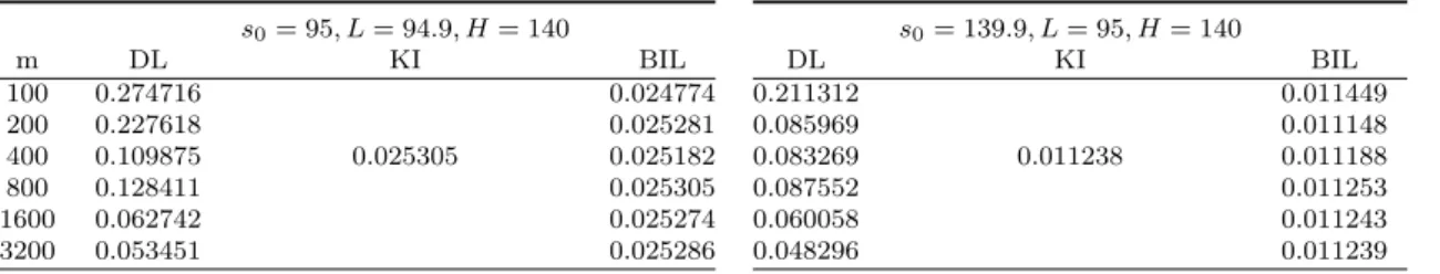
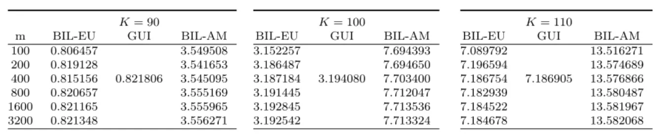
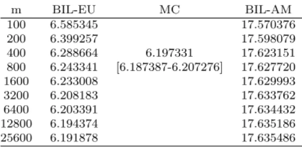
In Section 2.8 numerical results obtained with the BIL algorithm are given and compared with the closed-form formulas provided in Guillaume ([43], 2010) in the case of 2-step double knock-out put options. The American option prices calculated with our method have no benchmark value for the comparison. We also propose two numerical experiments for pricing 16-step double knock out put options. In the European case we use as a benchmark value the price given by the Monte Carlo method in Baldi, Caramellino and Iovino ([9], 1999) with 10 millions simulations and 1000 Euler time discretization steps. As for the 2-step case no benchmark is available for the American case.
2. Barrier options on discontinuous payoff functions
The study of the rate of convergence for the BIL algorithm requires the knowledge of the behavior of the classical CRR binomial approximation scheme for barrier-type options (see Proposition 2.6.1). To be precise, ifn ∈N denotes the number of time steps of the tree, we need to know the asymptotic expansion of the CRR binomial approximation error that is defined as
ErrCRR(n) = priceCRR(n)−priceBS, (0.0.8)
where priceCRR(n) denotes the price calculated by using the CRR tree scheme.
For standard (i.e.without barriers) call options it is known that the main term in (0.0.8) is of order 1n (see for example Diener and Diener ([31], 2004) and Chang and Palmer ([20], 2007)). For standard digital options the expression in (0.0.8) has a contribution of order √1
n related
to the position of the discontinuity point of the payoff function (K for digital options) and for this result one can refer to Walsh and Walsh ([82], 2004) and Chang and Palmer ([20], 2007).
that gives an upper bound of the binomial approximation error (0.0.8) for a general class of continuous payoff functions with double barriers by using PDE techniques, see Section 1.2.2. He finds that the quantity in (0.0.8) is the sum of two terms of order √1
n related to the
distance in the tree structure between the contractual barriers and the effective ones plus a term Rn such that there exist a constant C >0 s.t. |Rn| ≤Clognn.
A very recent result for call options with a single barrier is the one given in Lin and Palmer ([62], 2013). Here the authors give an explicit asymptotic expansion of (0.0.8). They use a different approach that consists in writing the CRR binomial price in terms of binomial coefficients as in Reimer and Sandmann ([70], 1995) and then approximating it through the normal distribution. In agreement with the upper bound given in Gobet ([42], 2001), they find a contribution of order √1
n related to the position of the contractual barrier with respect
to the nodes of the tree.
The results known from the literature concerning the analysis of the quantity in (0.0.8) when dealing with barrier options always require the continuity on the payoff function (Gobet ([42], 2001), Lin and Palmer ([62], 2013)). On the other hand when the payoff is assumed to be discontinuous the analysis of the rate of convergence of the binomial algorithm is given only for vanilla options (Walsh and Walsh ([82], 2002), Chang and Palmer ([20], 2007)). This is the reason why we decided to give our contribution in order to study theoretically and numerically barrier options on discontinuous payoff functions. In particular we deal with the simplest case of digital call options (the case of digital put options being similar), that can be used to generalize the treatment to the case of generic discontinuous payoff functions with a finite number of discontinuity points.
A digital call option is an option where the payoff is equal to a fixed amount (in what follows we suppose this amount is equal to 1) if the underlying asset at maturity is greater than a predetermined level (the strike priceK) or nothing otherwise. Practitioners that trade these products essentially predict the direction of the market without concerning in the specific the magnitude of the movements of the underlying asset price. One of the benefits with respect to standard products is that the investment and the returns are fixed, so the risk involved and the potential losses are known a priori.
Digital options can also include barrier levels. This more complex option can be used as a financial tool embedded in sophisticated products, such as accrual range notes. These notes are financial securities that are linked for example to a foreign exchange rate and then they pay a fixed interest accrual if the exchange rate remains within a specified range and nothing otherwise (see Wystup ([86], 2006) and also Hui ([48], 1996)).
We treat the option pricing problem related to these options by using lattice techniques. In order to do this we first need to find an asymptotic expansion of the binomial approximation error (0.0.8) and then we set up an algorithm such that it behaves “well”, in the sense that the worst contribution in (0.0.8) (which is of order √1
n) is nullified. In particular we treat
the study of the error (0.0.8) in the following two cases: digital options with a single barrier and digital options with double barriers. In the first case we get a complete theoretical result that allow us to construct an efficient algorithm, in the second one we obtain a partial theoretical result and we are able to make some numerical experiments on which we can
make some conjectures. We now describe our contribution in more details.
First of all we find an explicit asymptotic expansion of the binomial approximation error for digital call options with a single barrier, see Section 3.1. It turns out that the contribution of order √1
n in (0.0.8) is due both to the position of the barrier and also to the position of
the strike price with respect to the nodes of the tree. For this theoretical result we follow the techniques in Chang and Palmer ([20], 2007) and Lin and Palmer ([62], 2013). We stress here that the objective in [20] and [62] is to speed up the convergence of the CRR algorithm by explicitly calculating the terms of order √1
n and then subtracting them to (0.0.8) in order to
get an algorithm of order n1. Instead, we want to set directly a numerical procedure such that the contribution of order √1
n is nullified. This can be done by adjusting the BIL algorithm
to this specific case. In fact if the binomial mesh is constructed such that the lower barrier lies exactly on a node of the tree at maturity and the strike is located halfway between two nodes at maturity then, according to the theoretical result we obtained, we get an algorithm of order 1n. This is enhanced with the numerical experiments in Section 3.3.1.
The treatment of double barrier digital options is not straightforward. In fact no manageable binomial closed-form formulas exist in general for double barrier options and then we cannot proceed as for the single barrier case. But by using a PDE approach as described in Gobet ([42], 2001) we are able to get an upper bound of the binomial approximation error for double barrier options with a general discontinuous payoff function, but we stress here that our contribution is still partial at the moment. In Section 3.3.2 of the numerical results we propose some experiments on which we can formulate some conjectures.
3. Options on a model with CIR interest rate
In the last part of this thesis we study an efficient lattice method for option pricing when the underlying price process takes into account a stochastic interest rate. So we consider a generalization of the model (0.0.3): under the risk neutral probability measure, we assume that the underlying asset price (S(t))t∈[0,T] has the following dynamic:
dS(t) = r(t)S(t)dt+σSS(t)dZS(t), S(0) =s0 >0, (0.0.9)
where r is the short interest rate process, σS is the constant stock price volatility and ZS is
a standard Brownian motion. The risk-neutralized dynamic for the interest rate is described by the CIR model, i.e.
dr(t) =κ(θ−r(t))dt+σr
p
r(t)dZr(t), r(0) =r0 >0, (0.0.10)
whereκis the constant reversion speed,θis the long-term reversion target,σris the constant
interest rate volatility and Zr is a standard Brownian motion. We suppose that the two
Brownian noises ZS and Zr are correlated.
Starting from 1990, the introduction in financial markets of long-term options whose time to maturity is at least two years at the time of issue, such as LEAPS options (with LEAPS
standing for “Long-term Equity Anticipation Security”), involves the necessity of considering equity models with a stochastic interest rate, see for example Bakshi et al. ([7], 2000). We also observe that taking into account for stochastic interest rates is crucial for the pricing of forward starting options, i.e. options that start at a specified date in the future with an expiration date set further in the future. In fact securities with forward starting features often have long-dated maturities and are therefore much more interest rate sensitive, see Haastricht and Pelsser ([44], 2009).
Moreover, we also notice that some insurance products such as equity-linked policies with a minimum guaranteed need financial mathematics techniques in order to compute the fair premiums. These policies are products in which part of the capital spent for purchasing the policy is invested in a portfolio of equities whose performance influences the coverage of the insured. In fact at every premium payment date, the insurer can decide to continue the contract and then pay the premium again or surrender the contract and receive the maximum between the value of the fund of equities or a minimum guaranteed. Then these policies embed a Bermudan option, i.e. an option in which the buyer can exercise at a discrete set of dates before maturity. Since they are necessarily long-term contracts, it turns out to be convenient to describe the equity with a bivariate model in which the dynamic of the interest rate is stochastic, see for example Costabile et al. ([25], 2009) and Martire ([63], 2012).
The issue of pricing options with stochastic interest rate is then needed to be solved. Merton ([64], 1973) provides a closed-form formula for European options with interest rate following the Ornstein-Uhlenbeck process, but no expressions for the American counterpart are avail-able. We also observe that a more suitable model that guarantees the positivity of interest rates is given by the CIR process, then one should consider for the interest rate the dynamic given in (0.0.10), and in this specific case no closed-form formulas are available both for the European case and the American one.
Lattice models have been studied in the literature in order to deal with a 2-dimensional diffusion process with correlated Brownian motions as in (0.0.9)-(0.0.10). Wei ([83], 1996) and then Hilliard, Schwartz and Tucker ([46], 2004) provided a bivariate tree for dealing with a stochastic interest rate. Actually, in Wei the dynamic for the short rate is given by the Vasicek model and the extension of the Wei procedure to the CIR process is described in Costabile et al. ([25], 2006). However we still call “Wei procedure” the natural extension to the CIR process.
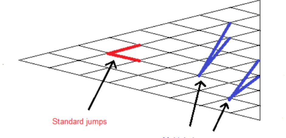
The idea in [83] and [46] is to extend to the 2-dimensional case a technique introduced by Nelson and Ramaswamy ([65], 1990) that consists in approximating 1-dimensional diffusion processes with computationally simple binomial processes. The original contribution of Nelson and Ramaswamy is the description of an approximating binomial process for a general class of diffusions such as (0.0.1), even if the coefficients present some singularities (as the diffusion coefficient of the CIR process). They introduce the so-called “multiple jumps” that allow the discrete process to have an up jump and a down jump but not necessarily on the two adjacent nodes of the tree as for the standard CRR model, see Figure 3. These jumps are specified such that some appropriate matching conditions on the local mean and the
Figure 3: Standard jumps and multiple jumps.
local variance between the discrete and the continuous process are satisfied.
We now briefly describe the generalization of the Nelson and Ramaswamy technique as proposed in Wei. The author suggests to construct a bivariate lattice by proceeding with the following four steps:
• transform both S and r into unit variance processes called ˜S and R respectively;
• define a new process Y as a function of ˜S and R that is orthogonal to R;
• model R and Y as two independent binomial processes following Nelson and Ra-maswamy and then merge the two structures into a 2-dimensional tree in which each node branches into four via joint probabilities that are simply obtained by product of the individual probabilities;
• at each node of the tree convert the variables R and Y back to r and S respectively and then proceed backwardly to obtain the option prices.
The procedure in Hilliard, Schwartz and Tucker is very similar to the one in Wei: they con-sider different transformations allowing one to deal with independent processes (see Section 4.3.2). So, what is important is the common idea to work with uncorrelated components that allow one to define the transition probabilities of the bivariate tree by means of products. Our algorithm (see Section 4.4) is structurally different from the previous ones in fact:
1. transformations similar to Wei and Hilliard, Scwhartz and Tucker are used but only to set up the state-space of the discrete approximation of the pair (S, r);
2. the probabilistic structure for the discrete approximation of bothS andras individual diffusions is defined directly on the original processes (using original drifts) and in this we recover the “original” idea in Nelson and Ramaswamy;
3. the transition probabilities of the bivariate lattice take in consideration the covariance structure (instead, the Wei and Hilliard, Schwartz and Tucker methods are strongly based on the use of a bivariate diffusion with components driven by uncorrelated noises).
Numerical results show that our method is robust and moreover it is not dependent on the choice of the input parameters, and this is a significant difference with respect to the procedure provided in [83] and [46], see Section 4.6. In fact in order to obtain the convergence in law of the tree built for the pair (S, r) we do not need to require the Feller condition, 2κθ ≥ σ2
r, or the so-called “convergence condition”, 4κθ ≥ σr2 (see Remark 4.4.1), but we
only need to assume that κ > 0 and θ > 0, that turn out to be natural requirements in a financial setting.
From a theoretical point of view we get two original results: the weak convergence of the tree method and the convergence of the prices given from the algorithm to their continuous counterparts.
Let us consider first the convergence of the scheme. Using standard techniques we prove in Section 4.5 the convergence on the Skorokhod space D([0, T];R2) of the c`adl`ag functions in
[0, T] with values in R2 of the tree method to the pair (S, r) solution of the SDE (0.0.9)-(0.0.10). It means that we set (Sh
i, rih)i=0,...,n the Markov chain running on the bivariate
lattice and then we set (Sht, rh
t)t∈[0,T] as the continuous time process defined through the
piecewise constant and c`adl`ag interpolations in time of the chain, that is:
Sht =Sih and rht =rih, ∀t ∈[ih,(i+ 1)h). (0.0.11) We observe that we could also define (Sht, rht)t∈[0,T] as the continuous time process obtained
by linearly interpolating in time the discrete Markov chain as in (0.0.2), in fact the two approaches are equivalent (see Theorem 1.1.4). But the choice of working in the space
D([0, T];R2) turns out to be more convenient in the second theoretical result, i.e. the
convergence of the prices.
Then we get that the family of Markov processes (Sh, rh)
h converges in law on the space D([0, T];R2) to the diffusion process (S, r) solution of the SDE (0.0.9)-(0.0.10), see Theorem 4.5.8.
Secondly, in Section 4.5.2 we discuss the convergence of European and American option prices computed with the lattice algorithm to their corresponding continuous values. The reasoning is immediate for the European prices when the payoff function is continuous and bounded. But an extension of a result proved in Amin and Khanna ([3], 1994) allows us to get the convergence of the American prices (and then also of European prices) in a more general set of conditions on the payoff function. In particular let f(t, x) : [0, T]×D([0, T])→ [0,+∞) denote a payoff function. Consider the following assumptions:
• (H1)fis a continuous function (in the product topology) and for everyx, y ∈D([0, T]) such that xs=ys for each s∈[0, t] then f(t, x) = f(t, y);
• (H2)there exists δ >1 and h∗ >0 s.t. suph<h∗E supt≤T|e −Rt
0r¯
h
Then under hypothesis (H1) and (H2) Amin and Khanna prove the convergence of the American prices evaluated on the tree approximation to the ones in the continuous-time model. But we can say more. In fact, suppose that f fulfills the following polynomial-growth condition: there exists C > 0 and γ >1 such that
sup
t∈T
|f(t, x)| ≤C(1 + sup
t∈T
|xt|γ). (0.0.12)
Then hypothesis (H1) and (0.0.12) guarantee the convergence of the American prices com-puted with our algorithm to the corresponding continuous-time values. In fact if (0.0.12) is true, then hypothesis (H2) is verified because we prove that for every p > 1 there exists
h∗ <1 such that sup h<h∗ E sup t≤T e−p Rt 0r¯ h sds( ¯Sh t) p <∞. (0.0.13)
We remark that this is a non trivial extension of the results in Amin and Khanna ([3], 1994), see Section 4.5.2.
A further study that we don’t treat in this thesis and that represents the objective of a future research is the analysis of the rate of convergence of the bivariate algorithm. We stress that in the literature results on this issue are available only for the CRR tree approximation also when the payoff function is sophisticated (as for barrier options). This study is what we actually do in Chapter 2 and Chapter 3 by using PDE techniques when the payoff function is generic and by using the normal approximation of the sum of binomial coefficients in the more specific case of call and put options. However, when the model is 2-dimensional, as the one in (0.0.9)-(0.0.10), the treatment is not straightforward and is worth to be done.
Mathematical background
In this Chapter we present some theoretical results that we will use in the rest of the thesis. In Section 1.1 we consider the problem of the convergence of Markov chains to diffusions and we state a classical theorem that can be used for proving that the continuous time process built from the Markov chain running on a lattice scheme weakly converges to a specific diffusion process. We also introduce the Nelson and Ramaswamy technique ([65], 1990) and a theorem due to Amin and Khanna ([3], 1994) on the convergence of the American option prices computed on a discretization scheme to their continuous-time values. This part will help us to prove the convergence results on the new bivariate scheme proposed in Chapter 4. In Section 1.2 we recall some known results on the rate of convergence of binomial tree schemes for standard options and for barrier-type options. In particular we present a theorem due to Gobet ([42], 2001) that we will apply in Chapter 2 for obtaining the rate of convergence of the new binomial scheme proposed. We also state the explicit binomial error formulas due to Chang and Palmer ([20], 2007) and Lin and Palmer ([62], 2013) that will help us in the development of the contribution we give on barrier options with discontinuous payoff functions in Chapter 3.
1.1
Convergence of Markov chains to diffusions
In this Section we briefly describe the results about the weak convergence of Markov chains to diffusions, as described in the books of Stroock and Varadhan ([74],1979), Kushner ([57],1977), Kushner and Dupuis ([58],1992), Ethier and Kurtz ([32],1986), Billingsley ([12], 1968) and also in the notes of Pag`es ([66],2001). We stress that here we use the notations adopted in Stroock and Varadhan ([74], 1979).
The basic idea is the following. Since we are concerned with computational techniques, the idea is to approximate the original stochastic process with a simpler approximating process that is a Markov chain on a finite state space. We remark that the finiteness of the approx-imating chain simplify the discussion in the theoretical results and it is indeed the case we are concerned with in the following chapters, but most of the theoretical results hold the same also if we remove this requirement. The approximating chain is parametrized by a
parameter h > 0, such that as the parameter goes to zero certain “local properties” of the approximating chain are consistent to the ones of the limit process. Under a set of broad conditions one can prove that the sequence of approximating chains converges in law to the continuous process as the approximation parameter goes to zero.
First we will present some technical results that allow us to prove the main theorem con-cerning the weak convergence of Markov chains to diffusions. We also briefly prove the well-known weak convergence of the CRR binomial scheme. Secondly, we will show the discrete approximation procedure due to Nelson and Ramaswamy ([65], 1990) and we will show that the sequence of Markov chains built from the discrete scheme they propose weakly converges to the original diffusion. Finally, we make some remarks on the convergence of European and American option prices by using a result due to Amin and Khanna ([3], 1994).
1.1.1
Weak convergence result
Let us start with a brief overview of the notion of weak convergence as presented in Billingsley ([12], 1968), that we will directly express in terms of our specific case of interest.
Let us suppose that (S,S) is a complete and separable metric space equipped with the Borel
σ-algebra. We give the following definition:
Definition 1.1.1. Let us suppose that {Ph}
h is a family of probability measures on (S,S).
The family {Ph}
h is said to converge weakly to a probability measure P if
Z
f(x)Ph(dx)→ Z
f(x)P(dx) (1.1.1)
for all f(·)∈ Cb(S), where Cb(S) denotes the class of all the bounded and continuous
real-valued functions on S. Then, if Xh and X are random variables and
Ph and P are the
measures on (S,S) induced by Xh and X respectively, then the weak convergence of {
Ph}h
to P is equivalent to the convergence of {Xh}h to X in distribution (denoted by Xh ⇒X).
There are a number of ways one can formulate the notion of weak convergence of probability measures, for more details see the Portmanteau Theorem 2.1 in [12].
Remark 1.1.2. The random variablesXh can be even defined on different probability spaces.
However, one can choose a common probability space for the random variables and define a sequence {Yh}h with Yh having the same law of Xh for every h, in such a way that
the convergence occurs almost surely. This is the content of the Skorokhod representation theorem (for details see for example Theorem 2.2.2 in Kushner ([57], 1937)).
Since it is not practical to prove the weak convergence of probability measures by directly using Definition 1.1.1, the idea is to show that the two following conditions are verified:
• the relative compactness of the family {Ph}
h, i.e. {Ph}h admits subsequential weak
• the uniqueness of the subsequential weak limit, i.e. if two different subsequences of
{Ph}
h converge toward a weak limit, then the limits must be the same.
In fact, if the family {Ph}
h is relatively compact and there exists one subsequential weak
limit P, then {Ph}
h weakly converges to P.
We remark that in complete and separable metric spaces the notion of relative compactness of measures reduces to its tightness (Prohorov’s Theorem 6.1 and 6.2 in [12]), that consists, roughly speaking, in the fact that the sequence of processes {Xh}
h (that induce on (S,S)
the family of probability measures {Ph}
h) does not oscillate too widely.
In the sequel we will specify our discussion to the case in which the complete and separable metric space isC([0,1];Rd) of the
Rd-valued continuous functions on the finite interval [0,1]
equipped with the metric of the sup-normρ that is defined as
ρ(x, y) = sup
t∈[0,1]
kx(t)−y(t)k, ∀x, y ∈ C([0,1];Rd).
Remark 1.1.3. Without lack of generality we work in the time interval [0,1], the case of a generic interval [a, b] with −∞ ≤a < b≤+∞ being similar. In particular, in Chapter 4 we will use the results presented in this Section when the time interval is [0, T], where T is the maturity date of the option.
Then we consider the problem of proving the weak convergence of a sequence of processes with trajectories in C([0,1];Rd) that we define in what follows to a given diffusion process
X. Let us describe the setup we will be working with (see Stroock and Varadhan ([74], 1979)).
Given x0 ∈Rd, let Πh(x,·) be a transition function on Rd. We assume that for every h >0
a discrete (in time and space) Markov chain (Xh
ih)i with associated transition probability Πh
and deterministic starting point x0 ∈Rd is given. It means that for eachh >0 we have:
• Ph(Xh 0 =x0) = 1; • Ph Xh (i+1)h ∈Γ|Mih = Πh(Xihh,Γ), (P−a.s.)∀i≥0,∀Γ∈ BRd,
where Mih = σ{Xkhh : 0 ≤ k ≤ i} and BRd is the Borel σ-field of subsets of R
d. So, the
previous two conditions mean that for everyh >0 the process (Xh
ih)i is a time-homogeneous
Markov chain starting from x0 with transition probability Πh(x,·). We also observe that
homogeneity is not really a necessary hypothesis but in practice we will be concerned with this specific case. Moreover, from the martingale formulation for discrete time processes (see [74] pages 165-166), the second condition is equivalent to say that
f(Xihh)− i−1 X j=0 Lh(f(Xjhh )),Mih,Ph !
is a discrete martingale for each f ∈C0∞(Rd), where L
h is the operator defined as follows Lhf(x) =
Z
and C0∞(Rd) is the set of all the C∞-functions f :
Rd → R having compact support. We
now define for each h a continuous-time process (Xh
t)t by linearly interpolating in time the
discrete Markov chain (Xihh)i, i.e.
Ph " Xth = (i+ 1)h−t h X h ih+ t−ih h X h (i+1)h, ih≤t <(i+ 1)h # = 1, ∀i≥0. (1.1.3)
Then, for every fixedh, (Xh
t)t is a continuous-time process with trajectories in C([0,1];Rd).
Another possibility is to define the process (Xh
t)tby piecewise c`adl`ag interpolations in time,
i.e. PhXth =X h ih, ih≤t <(i+ 1)h = 1, ∀i≥0. (1.1.4) In this case (Xh
t)t has trajectories in the space D([0,1];Rd) of the c`adl`ag functions with
values in Rd. This space turns out to be a complete and separable metric space when it is equipped with the Skorokhod metric (for details see Billingsley ([12], 1968) Chapter 4). The two approaches are equivalent, in fact the following Theorem holds:
Theorem 1.1.4. The sequence of processes defined in (1.1.3) with trajectories in the space
C([0,1];Rd)equipped with the sup-norm metric weakly converges towards a given continuous
process X if and only if the sequence of processes defined in (1.1.4) with trajectories in the space D([0,1];Rd) equipped with the Skorokhod metric weakly converges to X.
Remark 1.1.5. The space C([0,1];Rd) is a subset of D([0,1];Rd). Since the Skorokhod topology restricted to the space C([0,1];Rd) coincides with the uniform topology there, then
the weak convergence of processes with trajectories in C([0,1];Rd) implies that the processes
weakly converge as processes with trajectories in D([0,1];Rd). Furthermore, the weak con-vergence in D([0,1];Rd) towards a continuous process X implies the weak convergence in C([0,1];Rd) of the linear interpolations. So the two approaches are indeed equivalent and to
simplify the treatment we follow Stroock and Varadhan and we work in the spaceC([0,1];Rd). In fact, as explained in Billingsley ([12], 1968), the development of the same arguments in the spaceD([0,1];Rd) involves a characterization of the compact sets inD([0,1];
Rd)and the
study of criteria for the tightness and this requires much more technical results.
We now want to determine conditions under which the sequence of continuous-time processes
{Xh}
hwith corresponding probability measures{Ph}hconverges in distribution to a diffusion
process X that induces on C([0,1];Rd) the measure P and whose generator is
L= 1 2 d X i,j=1 ai,j(x) ∂2 ∂xi∂xj + d X i=1 bi(x) ∂ ∂xi , (1.1.5) in which b : Rd → Rd and a :
Rd → S(d), where S(d) denotes the set of all non-negative
that b and σ are continuous and locally bounded functions (see Chapter 6 in Stroock and Varadhan ([74], 1979)) then the following stochastic differential equation
dXt =b(Xt)dt+σ(Xt)dBt, X0 =x0 (1.1.6)
has a unique (in law)weak solution. It means that whenever two weak solutions of the SDE (1.1.6) have the same initial distribution, then they also have the same law.
Given the operator defined in (1.1.5) one can formulate the martingale problem associated toL as follows:
Definition 1.1.6. A solution to the martingale problem associated to L (or to b and a) starting from x0 ∈Rd is a probability measure P on the spaceC([0,1];Rd) equipped with the
Borel σ-algebra that satisfies the following two conditions: • P(X0 =x0) = 1;
• f(Xt)−
Rt
0 Lf(Xu)du is aP-martingale for all f ∈C
∞
0 (Rd) with respect to the natural
filtration {Ft}t.
We recall here that C0∞(Rd) is the space of all functions f : Rd → R having continuous derivatives of all orders and compact support.
Similarly to the discrete case, there exists a one-to-one correspondence between weak so-lutions of the SDE (1.1.6) and the martingale problem formulation (see Corollary 5.3.4 in Ethier and Kurtz ([32], 1986)).
In particular, we get the uniqueness in distribution of the solutions of the SDE (1.1.6) if and only if the solution to the martingale problem associated to L is unique, where in the martingale problem context uniqueness means that all the solutions with identical starting points have the same law on the path-space.
We now describe the main technical result that allows us to state the weak convergence as
h ↓0 of the sequence of Markov chains {Xh}
h defined in (1.1.3) to the diffusion process X
solution of the SDE (1.1.6).
We first need to define some quantities related {Xh}h that for every fixed h are:
ahi,j(x) = 1 h Z |y−x|≤1 (yi−xi)(yj−xj)Πh(x, dy), ∀i, j, bhi(x) = 1 h Z |y−x|≤1 (yi−xi)Πh(x, dy), ∀i, ∆h(x) = 1 hΠh(x,R d\B(x, )), ∀ >0.
It is clear that ah(·) and bh(·) are the local second moment and the local drift of the chain respectively and that ∆h
(·) represents a measure of the probability per unit of time of a
jump of size or greater than .
The main convergence result is the following (Theorem 11.2.3 in Stroock and Varadhan ([74], 1979)):
Theorem 1.1.7. Let us assume that for allR >0 and for all >0 the following conditions are true: lim h→0|supx|≤Rkah(x)−a(x)k= 0, (1.1.7) lim h→0|supx|≤R|bh(x)−b(x)|= 0, (1.1.8) lim h→0|supx|≤R∆ h (x) = 0, (1.1.9) where a: Rd→ S(d) and b :
Rd→ Rd are continuous functions. In addition, let us assume
that the coefficients a and b have the property that for each starting point x0 ∈ Rd the
martingale problem for a and b has exactly one solution P. Then {Ph}
h weakly converges to
P on C([0,1];Rd) as h → 0 uniformly on compact subsets of Rd, i.e. {Xh}h converges in
distribution to X.
Remark 1.1.8. We observe that conditions (1.1.7) and (1.1.8) require the convergence as
h→0of the local second moment and the local drift of the chain to the respective continuous counterparts. Moreover, condition (1.1.9) assumes that the probability ∆h
(·) goes to zero
and this is related to the fact that diffusion processes have sample paths that are continuous w.p. 1. We also remark that (1.1.7), (1.1.8), (1.1.9) are equivalent to the condition that for each f ∈C0∞(Rd)
1
hL
hf →Lf (1.1.10)
uniformly on compact subsets of Rd (for details see Lemma 11.2.1 in ([74], 1979)).
As explained at the beginning of this Section, in order to prove the weak convergence one needs to show that the family of probability measures {Ph}
h is relatively compact and that
there exists one subsequential weak limit P. The relative compactness is directly implied by conditions (1.1.7), (1.1.8), (1.1.9) because they are used to show that the sequence{Xh}
h is
tight (for details see Theorem 1.4.11 in [74]). Then, since the convergence condition (1.1.10) on the generators holds, it is immediate to deduce that the only possible weak subsequential limit of{Ph}
h solves the martingale problem associated to a andb and then it is indeed the
measure P induced on C([0,1];Rd) by the diffusion process X. But since the martingale
problem as a unique solution, then the desired conclusion follows.
1.1.2
Weak convergence of the CRR binomial tree
We now show that the conditions of Theorem 1.1.7 are satisfied by the classical binomial discretization scheme due to Cox, Ross and Rubinstein ([28], 1979), CRR hereafter. Let us suppose to fix the maturity time T >0. The CRR model is used to approximate the stock price process (Xt)t∈[0,T] in the Black and Scholes model, so under the risk-neutral measure
P∗ the processX is the solution of the following SDE
wherer is the risk free rate and σ the volatility parameter. We know that (Xt)t∈[0,T] can be
explicitly expressed as follows
Xt=x0e(r−
1 2σ
2)t+σB
t, ∀t ∈[0, T],
then we can introduce the process (Xt)t∈[0,T] of the log-return defined as
Xt = logXt, ∀t∈[0, T],
and so
Xt =X0+µt+σBt, with X0 = logx0 and µ=r−
1 2σ
2
.
Then the process (Xt)t∈[0,T] follows the SDE
dXt =µdt+σdBt. (1.1.12)
We set h = T /n, with n ∈ N, that is the constant time step of the binomial tree. Let us now denote with (Xhih)i=0,...,n the discrete in time and in space process corresponding to the
CRR binomial tree that is defined as
Xhih=X0+ i X j=1 ξjσ √ h, (1.1.13)
where (ξi)i=0,...,n are i.i.d. Bernouilli random variables such that
P(ξi = 1) =ph = 12 + 2µσ √ h, P(ξi =−1) = 1−ph = 12 − µ 2σ √ h.
Remark 1.1.9. We observe that the risk-neutral probabilityph in the original work of Cox,
Ross and Rubinstein ([28], 1979) is defined as
ph =
erh −e−σ
√
h
eσ√h−e−σ√h. (1.1.14)
If we make a Taylor expansion at the first order of the expression in (1.1.14), we get
ph = 1 2 + µ 2σ √ h+o(√h) (1.1.15)
and this is indeed the probability we use in practice.
First of all we observe that the coefficients µ and σ in (1.1.12) are constant, so they are continuous and there exist a unique solution to the martingale problem associated to µand
a =σ2. Let us now compute the local drift, that we call µ
h, and the local second moment,
that we denote withσ2
h, associated to the process (1.1.13). We get:
µh = 1 h[phσ √ h+ (1−ph)(−σ √ h)] =µ+ o(h) h ; σh2 = 1 h[ph(σ √ h)2+ (1−ph)(−σ √ h)2] =σ2+ o(h) h .
Then it is easy to see that conditions (1.1.7) and (1.1.8) of Theorem 1.1.7, that concern the uniform convergence on the compact subsets of R of the local drift µh and the local second moment σ2
h of the discrete process to µ and σ2, are verified. Moreover, since the space step
of the discrete scheme is σ√h, then condition (1.1.9) of Theorem 1.1.7 is true as well. Then the following result holds:
Theorem 1.1.10. The process Xh defined in (1.1.13) weakly converges to the diffusion process solution of (1.1.12).
1.1.3
Nelson and Ramaswamy technique for diffusion
approxima-tions
We now describe the technique in Nelson and Ramaswamy ([65], 1990) used to construct a computationally simple binomial process that weakly converges to a generic 1-dimensional diffusion. As pointed out by the authors, the term “binomial process” is indeed an abuse of terminology because it does not refer to a discrete process that follows a binomial distribution (as in Cox, Ross and Rubinstein ([28], 1979)), but more generally it is used for a two-state discrete model that we briefly call binomial tree. We remark that a tree is defined “computationally simple” if the number of nodes in the structure grows at most linearly in the number of time intervals (i.e. the lattice structure is path independent). This is a crucial feature of the approximating process because a computationally complex tree, such as a lattice in which the number of nodes increases not linearly, is useless for purposes such as option pricing.
Let us suppose to consider in the time interval [0, T] the stochastic differential equation (1.1.6) that is
dXt=b(Xt)dt+σ(Xt)dBt, X0 =x0.
First of all the interval [0, T] is divided into n subintervals of length h = T /n. For a fixed
h, (Xh
i,j)i,j for i = 0,1, ..., n, j = 0,1, ..., i is the binomial tree approximating the process X
defined with the following steps.
The first one is to turn the original SDE (1.1.6) into a new SDE with constant instantaneous volatility, that without lack of generality can be chosen equal to one. To this end, Nelson and Ramaswamy introduce a transformation g(x) ∈C2(R+) defined on the support of x as
follows
g(x) =
Z x 1
Then they define a new process Y by
Yt=g(Xt), ∀t∈[0, T]. (1.1.17) By Ito’s formula we get
dYt= ∂g(Xt) ∂x b(Xt) + 1 2σ 2(X t) ∂g(Xt) ∂x ! dt+dBt, =bY(Xt)dt+dBt, and Y0 =g(x0) =:y0.
The idea is to construct a binomial tree (Yh
i,j)i,j for i = 0,1, ..., n, j = 0,1, ..., i that
ap-proximates the processY and then to convert it back through the inverse transformation of (1.1.16) in order to get the binomial tree for X.
They now split the discussion in two cases: the first occurs when there are no singularities inσ(x), the second when there is a singularity at x= 0 such that σ(0) = 0 and b(0)≥0.
Case 1: no singularities in σ(x)
In this case they construct a computationally simple binomial approximation forY as follows:
• Y0h,0 =y0; • Yh i,j =y0+ (2j−i) √ h,∀j = 0, ..., i; • starting from Yh
i,j at time ih, the process Yh may jump at time (i+ 1)h to the two
following values
Yih+1,j+1 =Yi,jh +√h, Yih+1,j =Yi,jh −√h.
By using the inverse of (1.1.16) they now define a computationally simple tree (Xh
i,j)i,j for
the original process X as follows:
• Xh 0,0 =g −1(Yh 0,0) = x0; • Xh i,j =g −1(Yh i,j),∀j = 0, ..., i;
• starting from Xi,jh at time ih, the process Xh may jump at time (i+ 1)h to the two following values
Xih+1,j+1 =g−1(Yi,jh +√h), Xih+1,j =g−1(Yi,jh −√h).
The final step is to define the transition probabilities with which an up or a down jump occurs at each node of the tree. Such probabilities are chosen such that the local drift of the discrete process forX is exactly equal to the drift of the limiting diffusion (1.1.6), i.e.:
phi,j = b(g −1(Yh i,j))h+g −1(Yh i,j)−g −1(Yh i,j− √ h) g−1(Yh i,j+ √ h)−g−1(Yh i,j− √ h) . (1.1.18)
Since the quantity in (1.1.18) may not be a legitimate probability (it may not belong to [0,1]), they censor it as follows:
ph,i,j∗ = 0∨phi,j∧1. (1.1.19) Then the binomial scheme for the process X is given by:
Xi,jh =⇒ Xih+1,j+1, ph,i,j∗, Xh i+1,j, 1−p h,∗ i,j.
In order to prove the convergence of the discrete scheme (Xi,jh )i,j to the diffusion X, they
define a sequence of c`adl`ag Markov chains {Xih}i=0,1,...,n as in (1.1.4), i.e.:
• Xh
0 =x0;
• at timeih the state-space for Xih is given by
Xih ={Xi,jh , j = 0,1, ..., i};
• from timeih to time (i+ 1)h the transition law onR is given by
Ph(Xi,jh ;dx) =p h,∗ i,jδ{Xh i+1,j+1}(dx) + (1−p h,∗ i,j)δ{Xh i+1,j}(dx),
where δ{a} denotes here the Dirac mass in a ∈R.
As explained in Section 1.1, in order to guarantee the convergence in distribution of{Xh} h to X, one needs to prove conditions (1.1.7), (1.1.8) and (1.1.9) of Theorem 1.1.7. We suppose here that b and σ are suitable functions that guarantee the uniqueness of the martingale problem associated to b and a=σ2.
Let us define A∗ ={(i, j) :Xh
i,j ≤A∗}. Moreover let us call the local moment of order l at
time ih as Mi,j(l) =E((Xih+1−X h i ) l| Xih =Xi,jh )), l = 1,2,4,
where to simplify the notations we write E instead ofEPh.
First of all we need to prove the convergence of the local drift, i.e.: lim
h→0(i,jsup)∈A∗
1
h|Mi,j(1)−b(X h
But we have that Mi,j(1) =p h,∗ i,j(g −1 (Yi,jh +√h)−g−1(Yi,jh)) + (1−ph,i,j∗)(g−1(Yi,jh −√h)−g−1(Yi,jh)),
and by using (1.1.18) we get that Mi,j(1) =b(Xi,jh )h, then (1.1.20) easily follows.
Then we need to prove the convergence of the local diffusion coefficient,i.e.: lim
h→0(i,jsup)∈A∗
1 h|Mi,j(2)−σ 2 (Xi,jh )h|= 0. (1.1.21) We have that Mi,j(2) =ph, ∗ i,j(g −1(Yh i,j + √ h)−g−1(Yi,jh))2 + (1−ph,i,j∗)(g−1(Yi,jh −√h)−g−1(Yi,jh))2,
and by using a Taylor expansion at the first order we get that
g−1(Yi,jh ±√h) = g−1(Yi,jh)±σ(Xi,jh )
√
h+O(h), (1.1.22)
so that
Mi,j(2) =σ2(Xi,jh )h+O(h)
and then (1.1.21) easily follows.
Finally we need to prove the fast convergence to 0 of the fourth local moment, i.e. lim
h→0(i,jsup)∈A∗
1
hMi,j(4) = 0, (1.1.23)
that implies condition (1.1.9) of Theorem 1.1.7. Since from the Taylor expansion (1.1.22) we essentially have that (g−1(Yh
i,j−
√
h)±g−1(Yh
i,j))4 behaves ash2, then (1.1.23) easily follows.
Case 2: σ(0) = 0 and b(0)≥0.
In this case Nelson and Ramaswamy define the lower limit for Y by lim
x→0g(x) = y
L .
Moreover they slightly modify the inverse transformation of (1.1.16) as follows:
g−1(y) =
x:g(x) = y, if y > yL,
0, otherwise. (1.1.24)
Then they allow in a restricted region near the lower bound, that we call [yL, yB], that
the transformed process Y jumps by a quantity greater than √h. So they construct a computationally simple binomial approximation for Y as follows:
• Yh 0,0 =y0; • Yh i,j =y0+ (2j−i) √ h,∀j = 0, ..., i;
• starting from Yi,jh at time ih, the process Yh may jump at time (i+ 1)h to the two following values Yih+1,ju, Yih+1,jd, with jd=
the greatest indexj∗ ∈[0, j] :
g−1(Yh i,j)−g −1(Yh i+1,j∗)≤b(g−1(Yi,jh))h; 0, otherwise. and ju =
the smallest indexj∗ ∈[j+ 1, i+ 1] :
g−1(Yh
i+1,j∗)−g−1(Yi,jh)≥b(g−1(Yi,jh))h;
i+ 1, otherwise.
Then the process Yh may jump for a quantity greater than √h and it is not constrained
to necessarily reach the two adjacent nodes as in the classical CRR tree, so jd and ju are
called “multiple jumps”. We remark that in order to get computational simplicity, one needs to define multiple jumps just in a restricted region near the lower bound, otherwise the number of nodes might increase too fast. So, ifYi,jh > yB it is assumed that the binomial discretization for the process Y behaves as in Case 1.
By using (1.1.24) they get a computationally simple tree (Xh
i,j)i,j for the original processX:
• Xh 0,0 =g −1(Yh 0,0) = x0; • Xh i,j =g −1(Yh i,j),∀j = 0, ..., i;
• starting from Xi,jh at time ih, the process Xh may jump at time (i+ 1)h to the two following values Xih+1,j u =g −1(Yh i+1,ju), X h i+1,jd =g −1(Yh i+1,jd).
The transition probabilities are now defined as
phi,j = b(g −1(Yh i,j))h+g−1(Yi,jh)−g−1(Yih+1,jd) g−1(Yh i+1,ju)−g −1(Yh i+1,jd) . (1.1.25)
We remark that the quantities in (1.1.25) belong to [0,1] as a consequence of howjd and ju
are defined. Then the binomial scheme for the process X is given by:
Xi,jh =⇒
Xih+1,ju, phi,j, Xih+1,jd, 1−phi,j.
In this case the weak convergence of the c`adl`ag Markov chain running on the lattice (Xh i,j)i,j
(built as in Case 1) towards the limit diffusionXis not straightforward. Once the martingale problem associated tob anda =σ2 has a unique solution, one possibility is to prove directly conditions (1.1.7), (1.1.8) and (1.1.9) of Theorem 1.1.7. Otherwise one can prove some additional properties on the diffusion coefficients b and σ, as explained in Theorem 3 in Nelson and Ramaswamy ([65], 1990).
Remark 1.1.11. The advantage of the procedure proposed by Nelson and Ramaswamy is that it is constructive and, moreover, it can be applied to a generic diffusion process without restrictions on the parameters and also without requiring homogeneous coefficients (for the general case see [65]).
Remark 1.1.12. In Chapter 4 we will use the Nelson and Ramaswamy technique as in case 2 for the construction of a computationally simple binomial process for the CIR process, i.e. a process that follows the SDE
dXt=κ(θ−Xt)dt+σ
p
XtdBt, X0 =x0.
We will prove directly that conditions (1.1.7), (1.1.8) and (1.1.9) of Theorem 1.1.7 are verified (see Theorem 4.5.8). Moreover, we will be able to explicitly write the region in which multiple jumps may happen (see Lemma 4.5.1). We remark that an analogous procedure can be used for the discretization of the CEV (Constant Elasticity of Variance) process, i.e. a process that follows the SDE
dXt=κ(θ−Xt)dt+XtγdBt, X0 =x0,
withγ ∈[12,1]. By using techniques similar to the ones used in Chapter 4, it could be possible to prove also in this case the convergence conditions (1.1.7), (1.1.8) and (1.1.9) of Theorem 1.1.7.
1.1.4
Convergence of the American prices
Since the seminal work of Cox, Ross and Rubinstein ([28], 1979), discrete-time models have become really popular in option valuation because they represent a useful computational tool that can approximate the continuous-time diffusion model when no simple closed-form solutions are available. From a practical point of view, it is important to obtain that the sequence of American option prices computed with respect to the discrete-time model con-verges to the corresponding continuous-time American option value determined from the continuous-time diffusion process.
Let us assume to work in the setup described in Section 1.1 with the time interval [0,1] replaced by the interval [0, T], where T denotes the maturity time of the option.
The stock price process X follows the SDE (1.1.6) and we assume that for every h > 0, a discrete (in time and in space) Markov chain Xh approximatingX is given. Then we denote