Contents lists available atScienceDirect
Theoretical Computer Science
journal homepage:www.elsevier.com/locate/tcs
Stability analysis of the reproduction operator in bacterial
foraging optimization
Arijit Biswas
a, Swagatam Das
a, Ajith Abraham
b,∗, Sambarta Dasgupta
aaDepartment of Electronics and Telecommunication Engg, Jadavpur University, Kolkata, India
bMachine Intelligence Research Labs (MIR Labs), Scientific Network for Innovation and Research Excellence, USA
a r t i c l e i n f o
Keywords:
Foraging based optimization Bacterial foraging Reproduction Selection Global optimization Computational chemotaxis
a b s t r a c t
In his seminal paper published in 2002, Passino pointed out how individual and groups of bacteria forage for nutrients and how to model it as a distributed optimization process, which he named the Bacterial Foraging Optimization Algorithm (BFOA). One of the major operators of BFOA is the reproduction phenomenon of virtual bacteria, each of which mod-els one trial solution of the optimization problem. During reproduction, the least healthy bacteria (with a lower accumulated value of the objective function in one chemotactic life-time) die and the other healthier bacteria each split into two, which then starts exploring the search place from the same location. The phenomenon has a direct analogy with the selection mechanism of classical evolutionary algorithms. This paper attempts to model re-production as a dynamics and then analyses the stability of the reproductive system very near to an equilibrium point, which in this case is an isolated optimum. It also finds condi-tions under which a stable reproduction event can take place, to direct a worse bacterium towards a better one. Our analysis reveals that a stable reproduction event contributes to the quick convergence of the bacterial population near optima.
©2010 Elsevier B.V. All rights reserved.
1. Introduction
To tackle several complex search problems of real world, scientists have been looking into nature for years – both as a model and as a metaphor – for inspiration. Optimization is at the heart of many natural processes like Darwinian evolution, group behavior of social insects and the foraging strategy of other microbial creatures. Natural selection tends to eliminate species with poor foraging strategies and favor the propagation of genes of species with successful foraging behavior, as they are more likely to enjoy reproductive success.
Since a foraging organism or animal takes necessary action to maximize the energy accumulated per unit time spent for foraging, considering all the constraints presented by its own physiology such as sensing and cognitive capabilities, environment (e.g. density of prey, risks from predators, physical characteristics of the search space), the natural foraging strategy can lead to optimization and essentially this idea can be applied to real-world optimization problems [18,29,33]. Based on this conception, Passino proposed an optimization technique known as Bacterial Foraging Optimization Algorithm (BFOA) [1–3]. Till date, the algorithm has successfully been applied to real-world problems like optimal controller design [1,2], harmonic estimation [4], transmission loss reduction [5], pattern recognition [6], controller synthesis for active power filters [7] and power system optimization [8,32]. BFOA is a newly added member in the coveted realm of Swarm
∗Corresponding author.
E-mail addresses:[email protected](A. Biswas),[email protected](S. Das),[email protected](A. Abraham),
[email protected](S. Dasgupta). URL:http://www.mirlabs.org(A. Abraham).
0304-3975/$ – see front matter©2010 Elsevier B.V. All rights reserved.
Intelligence [9,10], which also includes powerful optimization techniques like the Particle Swarm Optimization (PSO) [10,11] and Ant Colony Optimization (ACO) [12].
One of the major steps of BFOA is the event of reproduction in which the bacterial population is at first sorted in order of ascending accumulated cost (value of the objective function to be optimized), then the worse half of the population containing least healthy bacteria is liquidated while all the members of the better half is split into two bacteria which start exploring the search space from the same location on the fitness landscape [30,31,34,35]. As pointed out by Passino, this phenomenon finds analogy with the elitist-selection mechanism of the classical evolutionary algorithms (EA) [1,2,13]. Bacteria in the most favorable environment (i.e., near an optima) gain a selective advantage for reproduction through the cumulative cost.
This paper provides a simple mathematical analysis of the reproduction mechanism in BFOA. We focus our attention on a simple two-bacterial system working over a one dimensional fitness landscape and try to model the reproduction event as a dynamics [14]. The resultant dynamics is then represented in a state space, where the displacement and velocity of a bacterium are assumed to be the state variables. We undertake a stability analysis of the reproduction event, very near to an isolated equilibrium point by linearizing the non-linear dynamics with Jacobian matrices. The analysis finds the relative positions of the two bacteria for which only a stable reproduction event can take place for accelerating the convergence.
The rest of the paper is organized as follows. Section2provides a comprehensive outline of the BFOA. Section3briefly surveys the existing literature on the research works undertaken on and with BFOA in recent past. In Section4we derive the mathematical model of the reproduction operator in BFOA. Then the stability analysis of the obtained dynamics is carried out in Section5. Finally Section6concludes the article and also uncovers some avenues for future research.
2. The bacterial foraging optimization algorithm
During foraging of the real bacteria, locomotion is achieved by a set of tensile flagella. Flagella help anEscherichia coli bacterium to tumble or swim, which are two basic operations performed by a bacterium at the time of foraging [1]. When they rotate the flagella in the clockwise direction, each flagellum pulls on the cell. That results in the moving of flagella independently and finally the bacterium tumbles with lesser number of tumbling whereas in a harmful place it tumbles frequently to find a nutrient gradient. Moving the flagella in the counterclockwise direction helps the bacterium to swim at a very fast rate. In the above-mentioned algorithm the bacteria undergoes chemotaxis, where they like to move towards a nutrient gradient and avoid noxious environment. Generally the bacteria move for a longer distance in a friendly environment. When they get food in sufficient, they are increased in length and in presence of suitable temperature they break in the middle to from an exact replica of itself. This phenomenon inspired Passino to introduce an event of reproduction in BFOA. Due to the occurrence of sudden environmental changes or attack, the chemotactic progress may be destroyed and a group of bacteria may move to some other places or some other may be introduced in the swarm of concern. This constitutes the event of elimination-dispersal in the real bacterial population, where all the bacteria in a region are killed or a group is dispersed into a new part of the environment.
Now suppose that we want to find the minimum ofJ
(θ)
whereθ
∈ <
p(i.e.θ
is ap-dimensional vector of real numbers), and we do not have measurements or an analytical description of the gradient∇
J(θ)
. BFOA mimics the four principal mechanisms observed in a real bacterial system: chemotaxis, swarming, reproduction, and elimination-dispersal to solve this non-gradient optimization problem. Below we introduce the formal notations used in BFOA literature and then provide the complete pseudo-code of the BFO algorithm. A more detailed description of the steps of BFOA is out of the scope of this article and can be found in [1].Let us define a chemotactic step to be a tumble followed by a tumble or a tumble followed by a run. Letjbe the index for the chemotactic step. Letkbe the index for the reproduction step. Letlbe the index of the elimination-dispersal event. Also let
p: Dimension of the search space,
S: Total number of bacteria in the population, Nc: The number of chemotactic steps, Ns: The swimming length.
Nre: The number of reproduction steps,
Ned: The number of elimination-dispersal events, Ped: Elimination-dispersal probability,
C
(
i)
: The size of the step taken in the random direction specified by the tumble.LetP
(
j,
k,
l)
= {
θ
i(
j,
k,
l)
|
i=
1,
2, . . . ,
S}
represent the position of each member in the population of theSbacteria at thejth chemotactic step,kth reproduction step, andlth elimination-dispersal event. Here, letJ(
i,
j,
k,
l)
denote the cost associated with the location of theith bacteriumθ
i(
j,
k,
l)
∈ <
p(sometimes we drop the indices and refer to theith bacterium position asθ
i). Note that we will interchangeably refer toJas being a ‘‘cost’’ (using terminology from optimization theory) and as being a nutrient surface (in reference to the biological connections). For actual bacterial populations,Scan be very large (e.g.,S=
109), butp=
3. In our computer simulations, we will use much smaller population sizes and will keep the population size fixed. BFOA, however, allowsp>
3 so that we can apply the method to higher dimensional optimization problems. Below we briefly describe the four prime steps in BFOA. We also provide a pseudo-code of the complete algorithm thereafter.(i) Chemotaxis: This process simulates the movement of anE. colicell through swimming and tumbling via flagella. Suppose
θ
i(
j,
k,
l)
representsith bacterium atjth chemotactic,kth reproductive andlth elimination-dispersal step.C(
i)
is a scalar and indicates the size of the step taken in the random direction specified by the tumble (run length unit). Then in computational chemotaxis, the movement of the bacterium may be represented byθ
i(
j+
1,
k,
l)
=
θ
i(
j,
k,
l)
+
C(
i)
∆(
i)
p
∆T
(
i)
∆(
i)
,
(1)where∆indicates a unit length vector in the random direction.
(ii) Swarming: An interesting group behavior has been observed for several motile species of bacteria includingE. coliand Salmonella typhimurium, where stable spatio-temporal patterns (swarms) are formed in semisolid nutrient medium. A group ofE. colicells arrange themselves in a traveling ring by moving up the nutrient gradient when placed amidst a semisolid matrix with a single nutrient chemo-effecter. The cells when stimulated by a high level ofsuccinate, release an attractantaspartate, which helps them to aggregate into groups and thus move as concentric patterns of swarms with high bacterial density. The cell to cell signaling inE. coliswarm may be represented by the following function.
Jcc
(θ,
P(
j,
k,
l))
=
SX
i=1 Jcc(θ, θ
i(
j,
k,
l))
=
SX
i=1"
−
dattractantexp−
w
attractantp
X
m=1(θ
m−
θ
mi)
2!#
+
SX
i=1"
hrepellentexp
−
w
repellentp
X
m=1(θ
m−
θ
mi)
2!#
,
(2)whereJcc
(θ,
P(
j,
k,
l))
is the objective function value to be added to the actual objective function (to be minimized) to present a time varying objective function. The coefficientsdattractant, w
attractant,
hrepellent, andw
repellentcontrol the strength of the cell to cell signaling. More specificallydattractantis the depth of the attractant released by the cell,w
attractantis a measure of the width of the attractant signal (a quantification of the diffusion rate of the chemical),hrepellent=
dattractant is the height of the repellent effect (a bacterium cell also repels a nearby cell in the sense that it consumes nearby nutrients and it is not physically possible to have two cells at the same location), andw
repellentis a measure of the width of the repellent. For a detailed discussion on the functionJccplease see [1].(ii) Reproduction:The least healthy bacteria eventually die while each of the healthier bacteria (those yielding lower value of the objective function) asexually split into two bacteria, which are then placed in the same location. This keeps the swarm size constant.
(iv) Elimination and dispersal: To simulate this phenomenon in BFOA some bacteria are liquidated at random with a very small probability while the new replacements are randomly initialized over the search space.
Pseudo-code of BFOA Parameters:
[Step 1]Initialize parametersp
,
S,
Nc,
Ns,
Nre,
Ned,
Ped,C(
i)(
i=
1,
2. . .
S)
,θ
i.Algorithm:
[Step 2]Elimination-dispersal loop:l
=
l+
1[Step 3]Reproduction loop:k
=
k+
1[Step 4]Chemotaxis loop:j
=
j+
1[a] Fori
=
1,
2. . . ,
Stake a chemotactic step for bacteriumias follows. [b] Compute fitness function,J(
i,
j,
k,
l)
.Let,J
(
i,
j,
k,
l)
=
J(
i,
j,
k,
l)
+
Jcc(θ
i(
j,
k,
l),
P(
j,
k,
l))
(i.e. add on the cell-to cell attractant–repellent profile to simulate the swarming behavior) where,Jccis defined in (2).[c] LetJlast
=
J(
i,
j,
k,
l)
to save this value since we may find a better cost via a run.[d] Tumble: generate a random vector∆
(
i)
∈ <
pwith each element∆m(
i),
m=
1,
2, . . . ,
p,
being a random number uniformly distributed in the interval[−
1,
1]
.[e] Move: Let
θ
i(
j+
1,
k,
l)
=
θ
i(
j,
k,
l)
+
C(
i)
∆(
i)
p
∆T
(
i)
∆(
i)
.
This results in a step of sizeC
(
i)
in the direction of the tumble for bacteriumi.
[f] ComputeJ
(
i,
j+
1,
k,
l)
and letJ(
i,
j+
1,
k,
l)
=
J(
i,
j,
k,
l)
+
Jcc(θ
i(
j+
1,
k,
l),
P(
j+
1,
k,
l))
. [g] Swim(i) Letm
=
0 (counter for swim length).(ii) Whilem
<
Ns(if have not climbed down too long).•
Letm=
m+
1.•
IfJ(
i,
j+
1,
k,
l) <
Jlast(if doing better), letJlast=
J(
i,
j+
1,
k,
l)
and letθ
i(
j+
1,
k,
l)
=
θ
i(
j,
k,
l)
+
C(
i)
∆(
i)
p
∆T
(
i)
∆(
i)
.
And use this
θ
i(
j+
1,
j,
k)
to compute the newJ(
i,
j+
1,
k,
l)
as we did in [f].•
Else, letm=
Ns. This is the end of the while statement.[h] Go to next bacterium (i
+
1) ifi6=
S(i.e., go to [b] to process the next bacterium).[Step 5]Ifj
<
Nc, go to step 4. In this case continue chemotaxis since the life of the bacteria is not over.[Step 6]Reproduction:
[a] For the givenkandl, and for eachi
=
1,
2, . . . ,
S, let Jhealthi=
Nc+1
X
j=1
J
(
i,
j,
k,
l)
be the health of the bacteriumi(a measure of how many nutrients it got over its lifetime and how successful it was at avoiding noxious substances). Sort bacteria and chemotactic parametersC
(
i)
in order of ascending costJhealth(higher cost means lower health).[b] TheSrbacteria with the highestJhealthvalues die and the remainingSrbacteria with the best values split (this process is performed by the copies that are made are placed at the same location as their parent).
[Step 7] Ifk
<
Nre, go to step 3. In this case, we have not reached the number of specified reproduction steps, so we start the next generation of the chemotactic loop.[Step 8] Elimination-dispersal: Fori
=
1,
2, . . . ,
Swith probabilityPed, eliminate and disperse each bacterium (this keeps the number of bacteria in the population constant). To do this, if a bacterium is eliminated, simply disperse another one to a random location on the optimization domain. Ifl<
Ned, then go to step 2; otherwise end.3. Related works on BFOA
Since its advent in 2002, BFOA has attracted the researchers from diverse domains of knowledge. This resulted into a few variants of the classical algorithm as well as many interesting applications of the same to the real-world optimization problems. In 2002, Liu and Passino [2] incorporated a new functionJar
(θ)
in BFOA to represent the environment-dependent cell-to-cell signaling, such thatJar
(θ)
=
exp(
M−
J(θ)).
Jcc(θ),
whereMis a tunable parameter andJcc
(θ)
is given by (2). For swarming, they considered the minimization ofJ(
i,
j,
k,
l)
+
Jar(θ
i)
.In [15], Tang et al. model the bacterial foraging behaviors in varying environments. Their study focused on the use of individual based modeling (IbM) method to simulate the activities of bacteria and the evolution of bacterial colonies. They derived a bacterial chemotaxis algorithm in the same framework and showed that the proposed algorithm can reflect the bacterial behaviors and population evolution in varying environments, through simulation studies. Li et al. proposed a modified Bacterial Foraging Algorithm with Varying Population (BFAVP) [16] and applied the same to the Optimal Power Flow (OPF) problems. Instead of simply describing chemotactic behavior into BFOA as done by Passino [1], BFAVP also incorporates the mechanisms of bacterial proliferation and quorum sensing, which allow a varying population in each generation of bacterial foraging process.
Tripathy and Mishra proposed an improved BFO algorithm for simultaneous optimization of the real power losses and Voltage Stability Limit (VSL) of a mesh power network [8]. In their modified algorithm, firstly, instead of the average value, the minimum value of all the chemotactic cost functions is retained for deciding the bacterium’s health. This speeds up the convergence, because in the average scheme described by Passino [1], it may not retain the fittest bacterium for the subsequent generation. Secondly for swarming, the distances of all the bacteria in a new chemotactic stage are evaluated from the globally optimal bacterium to these points and not the distances of each bacterium from the rest of the others, as suggested by Passino [1]. Simulation results indicated the superiority of the proposed approach over classical BFOA for the multi-objective optimization problem involving the UPFC (Unified Power Flow Controller) location, its series injected voltage, and the transformer tap positions as the variables. Mishra and Bhende used the modified BFOA to optimize the coefficients of Proportional plus Integral (PI) controllers for active power filters [7]. The proposed algorithm was found to outperform a conventional GA with respect to the convergence speed.
Mishra, in [4], proposed a Takagi–Sugeno type fuzzy inference scheme for selecting the optimal chemotactic step-size in BFOA. The resulting algorithm, referred to as Fuzzy Bacterial Foraging (FBF), was shown to outperform both classical BFOA and a Genetic Algorithm (GA) when applied to the harmonic estimation problem. However, the performance of the FBF crucially depends on the choice of the membership function and the fuzzy rule parameters [4] and there is no systematic method (other than trial and error) to determine these parameters for a given problem. Hence FBF, as presented in [4], may not be suitable for optimizing any benchmark function in general.
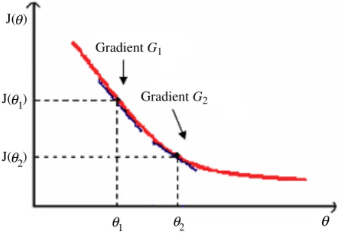
Gradient G1 J( ) Gradient G2 θ J( )θ1 θ1
θ
J( )θ2 θ2Fig. 1.A two-bacterium system on an arbitrary fitness landscape.
Hybridization of BFOA with other naturally inspired meta-heuristics has remained an interesting problem for the researchers. In this context, Kim et al. proposed a hybrid approach involving GA and BFOA for function optimization [3]. The proposed algorithm outperformed both GA and BFOA over a few numerical benchmarks and a practical PID controller design problem. Biswas et al. proposed a synergism of BFOA with another very popular swarm intelligence algorithm well known as the Particle Swarm Optimization (PSO). The new algorithm, named by the authors as Bacterial Swarm Optimization (BSO) [17], was shown to perform in a statistically significantly better way as compared to both of its classical counterparts over several numerical benchmarks. Dasgupta et al. derived a mathematical model for the chemotactic dynamics of BFOA and taking a cue from the analysis, they proposed an adaptation rule for the chemotactic step-size of BFO to promote quick convergence in [18].
Ulagammai et al. applied BFOA to train a Wavelet based Neural Network (WNN) and used the same for identifying the inherent non-linear characteristics of power system loads [19]. In [20], BFOA was used for the dynamical resource allocation in a multiple input/output experimentation platform, which mimics a temperature grid plant and is composed of multiple sensors and actuators organized in zones. Acharya et al. proposed a BFOA based Independent Component Analysis (ICA) [21] that aims at finding a linear representation of non-Gaussian data so that the components are statistically independent or as independent as possible. The proposed scheme yielded better mean square error performance as compared to a CGAICA (Constrained Genetic Algorithm based ICA). Chatterjee et al. reported an interesting application of BFOA in [22] to improve the quality of solutions for the extended Kalman Filters (EKFs), such that the EKFs can offer to solve simultaneous localization and mapping (SLAM) problems for mobile robots and autonomous vehicles.
To the best of our knowledge, none of the existing works has, however, attempted to develop a full-fledged mathematical model of the bacterial foraging strategies for investigating important issues related to convergence, stability and oscillations of the foraging dynamics near global optima. The present work may be considered as a humble contribution in this context.
4. Analysis of the reproduction step in BFOA
Let us consider a small population of two bacteria that sequentially undergoes the four basic steps of BFOA over a one-dimensional objective function. The bacteria live in continuous time and at thetth instant its position is given by
θ(
t)
. Below we list a few assumptions that were considered for the sake of gaining mathematical insight.4.1. Assumptions
(i) The objective functionJ
(θ)
is continuous and differentiable at all points in the search space.(ii) The analysis applies to the regions of the fitness landscape where gradients of the function are small i.e., near to the optima. The region of fitness landscapes between
θ
1andθ
2is monotonous at the time of reproduction.(iii) During reproduction, two bacteria remain close to each other and one of them must not superpose on another (i.e.
|
θ
2−
θ
1| →
0 may happen due to reproduction butθ
26=
θ
1. LetPandQ represent the respective positions of the two bacteria as shown inFig. 1). At the start of reproductionθ
1andθ
2remain apart from each other but as the process progresses they come close to each other gradually.(iv) The bacterial system lives in continuous time. 4.2. Analytical treatment
In our two bacterial system
θ
1(
t)
andθ
2(
t)
represent the position of the two bacteria at timetandJ(θ
1),
J(θ
2)
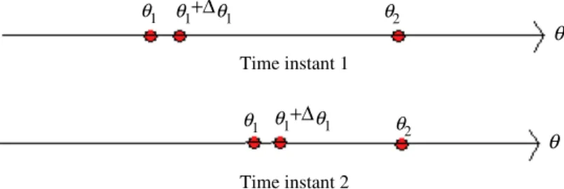
denote the cost function values at those positions respectively. During reproduction, the virtual bacterium with a relatively largerTime instant 1 Time instant 2
θ
θ
θ1 θ1 θ1 θ1 θ2 θ2+Δ
θ1+Δ
θ1Fig. 2.Change of position of the bacteria during reproduction.
value of the cost function (for a minimization problem) is liquidated while the other is split into two. These two offspring bacteria start moving from the same location. Hence in effect, through reproduction the least healthy bacteria shift towards the healthier bacteria. Health of a bacterium is measured in terms of the accumulated cost function value, possessed by the bacterium until that time instant. The accumulated cost may be mathematically modeled as
R
0tJ(θ
1(
t))
dt. For a minimization problem, higher accumulated cost represents that a bacterium did not get as many nutrients during its lifetime of foraging and hence is not as ‘‘healthy’’ and thus unlikely to reproduce. The two-bacterial system working on a single-dimensional fitness landscape has been depicted inFig. 1.To simulate the bacterial reproduction we have to take a decision on which bacterium will split in next generation and which one will die. This decision may be modeled with the help of the well-known unit step functionu
(
x)
(also known as Heaviside step function [23]), which is defined as,u
(
x)
=
1;
ifx>
0=
0;
otherwise.
(3)In what follows, we shall denote
θ
1(
t)
andθ
2(
t)
asθ
1andθ
2respectively. Now if we consider that1θ
1is the infinitesimal displacement (1θ
1→
0) of the first bacterium in infinitesimal time1t(
1t→
0)
towards the second bacterium in favorable condition i.e. when the second is healthier than the first one, then the instantaneous velocity of the first one is given by, 1θ11t. Now when we are trying to model reproduction we assume the instantaneous velocity of the worse bacterium to be proportional with the distance between the two bacteria, i.e. as they come closer their velocity decreases but this occurs unless we incorporate the decision making part. So, if the first bacterium is the worse one then,
1
θ
11t
∞
(θ
2−
θ
1)
⇒
1θ
11t
=
k(θ
2−
θ
1)
[where,kis the proportionality constant]⇒
1θ
11t
=
1.(θ
2−
θ
1)
=
(θ
2−
θ
1)
(4)[If we assume thatk
=
1 s−1].Since we are interested in modeling a dynamics of the reproduction operation, the decision making i.e. whether one of the bacteria will move towards the other, can not be discrete i.e. it is not possible to check straightaway whether the other bacterium is at a better position or not (Fig. 2). So a bacterium (suppose
θ
1) will be checking whether a position situated at an infinitesimal distance fromθ
1is healthier or not and then it will move. The health of first bacterium is given by the integral ofJ(θ
1)
from zero to timetand the same for the differentially placed position is given by the integral ofJ(θ
1+
1θ
1)
from zero to timet. Then we may model the decision making part with the unit step function in the following way:1
θ
1 1t=
uZ
t 0 J(θ
1)
dt−
Z
t 0 J(θ
1+
1θ
1)
dt·
(θ
2−
θ
1).
(5)Similarly, when we consider the second bacterium, we get, 1
θ
2 1t=
uZ
t 0 J(θ
2)
dt−
Z
t 0 J(θ
2+
1θ
2)
dt·
(θ
1−
θ
2).
(6)In Eq. (5),
R
0tJ(θ
1)
dtrepresents the health of the first bacterium at the time instanttandR
t0J
(θ
1+
1θ
1)
dtrepresents the health corresponding to(θ
1+
1θ
1)
at the time instantt. We are going to carry out calculations with the equation for bacterium 1 only, as the results for other bacterium can be obtained in a similar fashion.Since we are considering only the monotonous part of any function, so if
θ
2is at a better position, then any position, in-betweenθ
1andθ
2, has a lesser objective function value compared toθ
1. So we may concludeJ(θ
1+
1θ
1)
is less thanJ(θ
1)
. In that case we can imagine thatR
0tJ(θ
1+
1θ
1)
is less thanR
tu(x) 1 1 k=5 phi (x) k=10 k=infinity 0 x 0 x
Fig. 3.The unit step and the logistic functions.
is monotonous and change of
θ
1+
dθ
1with respect totis same as that ofθ
1. We write the Eq. (5) corresponding to bacterium 1 as, 1θ
1 1t=
u−
Z
t 0 J(θ
1+
1θ
1)
−
J(θ
1)
1t dt(θ
2−
θ
1).
[∵1t
>
0. We know for a positive constant1t,u(
1tx)
=
u(
x)
asxand1tx are of same sign and unit step function depends only upon sign of the argument.]⇒
Lt 1t→0 1θ1→0 1θ
1 1t=
1Ltt→0 1θ1→0 u−
Z
t 0 J(θ
1+
1θ
1)
−
J(θ
1)
1t dt·
(θ
2−
θ
1)
⇒
Lt 1t→0 1θ1→0 1θ
1 1t=
1Ltt→0 1θ1→0 u−
Z
t 0 J(θ
1+
1θ
1)
−
J(θ
1)
1θ
1 1θ
1 1t dt·
(θ
2−
θ
1).
Again,J
(θ)
is assumed to be continuous and differentiable.Lim1θ→0J(θ1+11θ1θ1)−J(θ1)is the value of the gradient at that point and may be denoted bydJ(θ1)dθ1 orG1. So we write,
⇒
dθ
1 dt=
u−
Z
t 0 dJ dθ
1 dθ
1 dt dt·
(θ
2−
θ
1)
[wheredθ1dt is the instantaneous velocity of the first bacterium]
⇒
v
1=
u−
Z
t 0 G1v
1dt·
(θ
2−
θ
1)
(7)[where
v
1=
ddθt1 andG1is the gradient ofJatθ
=
θ
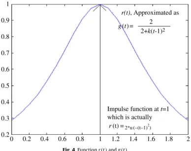
1.]Now in Eq. (5) we have not yet considered the fact that the event of reproduction is taking place att
=
1 only. So we must introduce a function of timer(
t)
=
2∗
u(
−
(
t−
1)
2)
(unit step) in product with the right hand side of Eq. (5). This provides a sharp impulse of strength 1 unit at timet=
1. Now it is well known thatu(
x)
may be approximated with the continuous logistic functionφ(
x)
[23,24], whereφ(
x)
=
11+e−kx. We note that, u
(
x)
=
Lt k→∞φ(
x)
=
Lt k→∞ 1 1+
e−kx.
(8)Fig. 3illustrates how the logistic function may be used to approximate the unit step function used for decision-making in reproduction. Note that if we use this approximation ofu
(
x)
withφ(
x)
, it follows that forx=
0,u(
0)
=
Ltk→∞φ(
x)
=
0.
5.In fact this is why (u
(
−
(
t−
1)
2)
) is multiplied with 2 in the above definition ofr(
t)
for gettingr(
t)
=
1 and not 0.5, when t=
1.Following this we may write: r
(
t)
=
2∗
u(
−
(
t−
1)
2)
≈
21 0.9 r(t), Approximated as Impulse function at t=1 which is actually r(t) =2*u (–(t–1)2 ) 0.8 0.7 0.6 0.5 0.4 0.3 0.2 0 0.2 0.4 0.6 0.8 1 1.2 1.4 1.6 1.8 2 g(t) = 2 2+k(t-1)2
Fig. 4.Functionr(t)andg(t).
For moderately large value ofk, sincet
→
1, we can have|
k(
t−
1)
2|
1 and thus ek(t−1)2≈
1+
k(
t−
1)
2. Using this approximation of the exponential term we may replace the unit step functionr(
t)
with another continuous functiong(
t)
whereg
(
t)
=
22
+
k(
t−
1)
2 (We can takek=
5)which is not an impulsive function just att
=
1 rather a continuous function as shown inFig. 4. Higher value ofkwill produce more effective result. Due to the presence of this function we see thatv
1(i.e,ddθt1) will be maximum att=
1 and decreases drastically when we move away fromt=
1 in both sides.So Eq. (7) is modified and becomes,
v
1=
u−
Z
t 0 G1v
1dt(θ
2−
θ
1)
·
2 2+
k(
t−
1)
2.
(9)For ease of calculation we denote the term within the unit step function asM
= −
R
t0G1
v
1dtto obtain,v
1=
u(
M)(θ
2−
θ
1)
·
22
+
k(
t−
1)
2.
(10)Sinceu
(
M)
=
Ltα→∞1+e1−αM.We take a smaller value of
α
for getting into the mathematical analysis (sayα
=
10). Since, we have the region, under consideration with very low gradient and the velocity of the particle is low, (so productG1v
1is also small enough), and the time interval of the integration is not too large (as the time domain under consideration is not large), so we can write, by expanding the exponential part and neglecting the higher order termsu
(
M)
=
11
+
(
1−
α
M)
=
12
(
1−
α
M/
2)
.
Putting this expression in Eq. (10) we get,
v
1=
1 2(
1−
α
M/
2)
(θ
2−
θ
1)
2 2(
1+
(
k/
2)(
t−
1)
2)
⇒
v
1θ
2−
θ
1(
1+
(
k/
2)(
t−
1)
2)
=
1 2 1+
α
M 2.
(11)[
∵|
θ
2−
θ
1| →
0 but|
θ
2−
θ
1| 6=
0 also∵|
αM2
|
1, neglecting higher order terms,(
1−
αM
2
)
−1
≈
(
1+
αM2
)
]Now the equation given by (11) is true for all values possible values oft, so we can differentiate both sides of it with respect totand get,
⇒
(θ
2−
θ
1)
dv1 dt−
v
1(
ddθt2−
dθ1 dt)
(θ
2−
θ
1)
2(
1+
(
k/
2)(
t−
1)
2)
+
v
1θ
2−
θ
1 k(
t−
1)
=
1 4 d(α
M)
dt.
(12)Now, d(αd·tM)
=
d(−α Rt0v1G1dt)
dt
= −
αv
1G1 [by putting the expression forM and applying the Leibniz theorem [22] for differentiating integrals]. So from (12), we get,(θ
2−
θ
1)
ddvt1−
v
1(
ddθt2−
ddθt1)
(θ
2−
θ
1)
2(
1+
(
k/
2)(
t−
1)
2)
+
v
1θ
2−
θ
1 k(
t−
1)
= −
1 4αv
1G1.
Puttingdθ1 dt=
v
1and dθ2dt
=
v
2after some further manipulations (where we need to cancel out(θ
2−
θ
1)
, which we can do as|
θ
2−
θ
1| →
0 towards the end of reproduction but never|
θ
2−
θ
1| 6=
0 according to assumption (iii)), we get,d
v
1 dt= −
v
2 1θ
2−
θ
1−
v
1 k(
t−
1)
1+
(
k/
2)(
t−
1)
2+
α
G1(θ
2−
θ
1)
4(
1+
(
k/
2)(
t−
1)
2)
−
v
2θ
2−
θ
1⇒
dv
1 dt= −
Pv
2 1−
Qv
1 (13) where,P=
θ 1 2−θ1 andQ=
(
k(t−1) 1+(k/2)(t−1)2+
αG1(θ2−θ1) 4(1+(k/2)(t−1)2)−
v2 θ2−θ1)
. 4.3. Physical significance of the modelSince the rate of change of velocity of bacterium 1 and 2 are dependent on
(θ
2−
θ
1)
and(θ
1−
θ
2)
respectively, it is evident that the distance between the two bacteria guides their dynamics. If we assume,θ
2> θ
1and they don’t traverse too long, the first bacterium is healthier (less accumulated cost) than the second one, when the function is decreasing monotonically in a minimization problem and also the time rate change of first bacterium is less than that of the second.So at the time of reproduction, in a two bacteria system, the healthier bacterium when senses that it is in a better position compared to its fellow bacterium, it hopes that the optima might be very near so it slows down and its search becomes more fine-tuned. This can be compared with the real bacterium involved in foraging. Whenever it senses that food might be nearby then it obviously slows down and searches that place thoroughly at cost of some time [25–27].
The second bacterium moves away from that place with a high acceleration quite naturally getting the information from the first bacterium that the fitter place is away from its present position. In biological system for grouped foraging when one member of the group share information from its neighbors it tries to move towards the best position found out by the neighboring members [26,27]. Thus we see that reproduction was actually included in BFOA in order to facilitate grouped global search, which is explained from our small analysis.
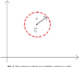
5. Stability analysis
In this section we undertake the stability analysis of the dynamics underlying the reproduction process (Fig. 5). A few related terms related to the stability analysis in classical control theory has been explained below.
Definition 5.1. A point
E
x= E
xeis called anequilibrium state,if the dynamics of the system is given by dE
xdt
=
f(
E
x(
t))
becomes zero at
E
x= E
xefor anyt i.e.f(
E
xe(
t))
=
0. The equilibrium state is also called equilibrium (stable) point inD -dimensional hyperspace, when the stateE
xehasD-components.Definition 5.2. State variablesare defined as the smallest possible subset of system variables that can represent the entire state of the system at any given time. State variables must be linearly independent; a state variable cannot be a linear combination of other state variables.
Definition 5.3. In control engineering, astate space representationis a mathematical model of a physical system as a set of input, output and state variables related by coupled first-order differential equations.
5.1. Stability conditions near equilibrium
Now for gaining further mathematical insight we do some simplifications over Eq. (13). The effect of reproduction is mostly pronounced aroundt
=
1, so(
t−
1)
→
0. Thus we can neglect the first expression inQ, which contains(
t−
1)
. Again we restrict our analysis to regions only where gradient is very low, i.e.,G1→
0. So we can also neglect the second expression inQ, which containsG1. Thus we get a simplified version of the acceleration of the first bacterium as,d
v
1 dt= −
v
2 1θ
2−
θ
1+
v
1v
2θ
2−
θ
1⇒
d 2θ
1 dt2=
dθ1 dt(v
2−
ddθt1)
(θ
2−
θ
1)
.
ε ε x
Fig. 5.The region in which our stability analysis is valid.
Now we will be undertaking a state variable analysis, Let us assume, thatx1andx2are two state variables, where x1
=
θ
1 and x2=
dθ
1 dt.
So we get,˙
x1=
x2=
f1(
x1,
x2)
(14) and x˙
2=
x2(v
2−
x2)
(θ
2−
x1)
=
f2(
x1,
x2).
(15)This is a nonlinear system and we want to perform the stability analysis of the system in a small region around the equilibrium point. Let
E
xe= [
x∗1,
x∗
2
]
be the equilibrium point of the system. Sof1(
x∗1,
x∗ 2
)
=
f2(
x∗1,
x ∗ 2)
=
0. Now,
dx1 dt=
f1(
x1,
x2)
=
f1(
x ∗ 1,
x ∗ 2)
+
∂
f1∂
x1 x1=
x∗1 x2=
x∗2(
x1−
x∗1)
+
∂
f1∂
x2 x1=
x∗1 x2=
x∗2(
x2−
x∗2).
(16) [by expanding with Taylor’s series around the equilibrium point]Similarly
,
dx2 dt=
f2(
x1,
x2)
=
f2(
x ∗ 1,
x ∗ 2)
+
∂
f2∂
x1 x1=
x∗1 x2=
x∗2(
x1−
x∗1)
+
∂
f2∂
x2 x1=
x∗1 x2=
x∗2(
x2−
x∗2).
(17) Let,p=
x1−
x∗1andq=
x2−
x∗2⇒
dp dt=
dx1 dt and dq dt=
dx2 dt.
From (16), dp dt=
∂
f1∂
x1 x1=
x∗1 x2=
x∗2 p+
∂
f1∂
x2 x1=
x∗1 x2=
x∗2 q[
∵f1(
x∗1,
x ∗ 2)
=
f2(
x∗1,
x ∗ 2)
=
0]
dq dt=
∂
f2∂
x1 x1=
x∗1 x2=
x∗2 p+
∂
f2∂
x2 x1=
x∗1 x2=
x∗2 q[
∵f1(
x∗1,
x ∗ 2)
=
f2(
x∗1,
x ∗ 2)
=
0]
.
Writing the above equations in a more compact form we get,
˙
p˙
q=
∂
f1 dx1∂
f1 dx2∂
f2 dx1∂
f2 dx2
−→ x=−→xe p q,
(18) whereJ=
"
∂f1 dx1 ∂f1 dx2 ∂f2 dx1 ∂f2 dx2#
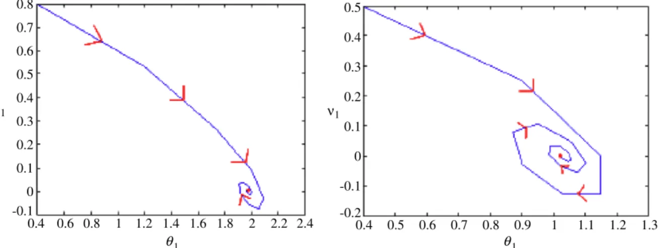
− → x=−→xe0.8 0.7 0.6 0.5 0.4 0.3 ν1 ν1 1 0.2 0.1 0 -0.1 0.8 0.6 0.4 1 1.2 1.4 1.6 1.8 2 2.2 2.4 θ θ1 0.5 0.4 0.3 0.2 0.1 0 -0.1 -0.2 0.8 0.9 1 0.7 0.6 0.5 0.4 1.1 1.2 1.3
Fig. 6.How the velocity and displacement of the first bacterium converge towards the equilibrium (red dot is the equilibrium point). (For interpretation of the references to colour in this figure legend, the reader is referred to the web version of this article.)
The eigenvalues of this Jacobian matrix are the poles of the linearized system. For stability of a system the poles must have negative real part [28]. Iff1andf2are given by Eqs. (14) and (15), then Eq. (18) becomes as,
˙
p˙
q=
0 1 x∗2(v
2−
x∗2)
(θ
2−
x∗1)
2(v
2−
2x∗2)
(θ
2−
x∗1)
p q,
(19)which is a linear state space representation of the nonlinear reproduction system around the equilibrium point. Let,M
=
x ∗ 2(v2−x∗2) (θ2−x∗1)2 andN=
(v2−2x ∗ 2) (θ2−x∗1), thenJmatrix looks like, J
=
0 1 M N.
Both of the eigenvalues of this matrix are real and they are,
λ
1=
−
2x∗ 2(θ
2−
x∗1)
andλ
2=
2(v
2−
x∗2)
(θ
2−
x∗1)
.
Now we are to determine whenf1
(
x1,
x2)
=
f2(
x1,
x2)
=
0, i.e., equilibrium values of the two state variables. We find that atx∗2
=
0 is a solution at which the system is in equilibrium, as then the rate of change of both the state variables becomes zero. Whenx∗2
=
0, we haveλ
1=
0 andλ
2=
(θ22−v2x∗1).For
λ
2<
0, (for system stability it is urgently required), we have two options, either (v
2<
0 andθ
2>
x∗1) or (v
2>
0 andθ
2<
x∗1). But in any caseλ
1is zero, which ensures a constant component of the state variables even in the final stage. So to assure full stability, we must haveSituation 1: (x∗
2
= +
ε
,v
2<
0 andθ
2>
x∗1) or Situation 2: (x∗2
= −
ε
,v
2>
0 andθ
2<
x∗1).That means at equilibrium the first bacterium should have an infinitesimal amount of positive or negative velocity to ensure stability of this reproductive system. InFig. 6we show two different probable phase trajectories (distance and velocity of first bacterium being the two variables) for a stable reproduction. It is evident from this figure that the final velocity is reduced to zero and the first bacterium comes to rest.
Now situation 1 is true when the second bacterium is in the part of the fitness landscapes where the slope is positive and the situation 2 is valid where the second one is on negative sloped fitness landscape part [since in the positive sloped part, velocity
v
2can never be positive and in the negative sloped part, velocityv
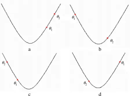
2can never be negative, as BFOA is a greedy search]. Case I corresponds to situation I and case II corresponds to situation II.Case 1: Both bacteria are in the same slope of the fitness landscape (Fig.7(a) and (b)):
In both the cases
θ
2>
x∗1(∼
=
x1) and we observe that in7(a) second bacterium is eventually less fit and as a result of it first bacterium never undergoes reproduction towards the other one. So the only possible case of reproduction in this scenario is7(b).Case I1: Both bacteria are in the opposite slope of the fitness landscape (Fig.7(c) and (d)):
In both the cases
θ
2<
x∗1(∼
=
x1) and now we see that in7(c) second bacterium is eventually less fit and as a result of it first bacterium never undergoes reproduction towards the other one. So the only possible case of reproduction in this scenario is7(d). So for stable and effective reproductive system bacterium must lie on fitness landscapes as shown inFig. 7(b) and (d).θ1 θ1 θ1 θ1 θ2 θ2 θ2 θ2
a
b
c
d
Fig. 7.Probable positions of the two bacteria.
Final position of bacterium 1 for stability
Trajectory followed by bacterium 1 during instability Error in final
positions due to
approximation Bacterium 2
Initial position of bacterium 1
Fig. 8.Stable and unstable situations in reproduction.
5.2. Unstable situation
The position of the second bacterium must be an equilibrium position with respect to the first bacterium, as the velocity of the first one must come down to almost zero at this place. If it does not stop here the main objective of reproduction step of bacterial foraging analysis will be violated. InFig. 8we try to depict, how the movement of first bacterium gets disturbed and misled for the case of unstable reproduction. The reproduction event was carried in BFOA to have a global search so that the worst bacterium can be guided towards the better bacterium, but here for instability the basic purpose of reproduction in BFOA is not fulfilled at all. In the same figure we also show a possible trajectory of the first bacterium towards the second one for a stable reproduction event.
6. Conclusions
This paper, the first of its kind, presents a mathematical analysis of the reproduction operator of the bacterial foraging optimization algorithm. First the reproduction step is modeled as a dynamics and then it is represented in a state space model. The model helps us to gain important insight into the search mechanism of the BFOA. On the basis of a stability
analysis performed on the derived model, we try to reach at some conclusions regarding the relative positions of the two bacteria in a one-dimensional two bacterial system, for which a stable reproduction event can take place. In the course of the bacterial foraging optimization process these relative positions enable us to make the system stable and effective according to our developed dynamics. We would like to point out that this work takes a significant step towards the mathematical analysis of BFOA, which appears as an attractive foraging theory based optimization technique of current interest. Future research should focus on extending the analysis presented here, to a group of bacteria working on a multi-dimensional fitness landscape and also include effect of the chemotaxis and elimination-dispersal events in the same. Deriving some control actions on the reproductive system model for eliminating the unstable behavior may be a worthy issue for future investigation.
References
[1] K.M. Passino, Biomimicry of bacterial foraging for distributed optimization and control, IEEE Control Systems Magazine (2002) 52–67.
[2] Y. Liu, K.M. Passino, Biomimicry of social foraging bacteria for distributed optimization: models, principles, and emergent behaviors, Journal of Optimization Theory And Applications 115 (3) (2002) 603–628.
[3] D.H. Kim, A. Abraham, J.H. Cho, A hybrid genetic algorithm and bacterial foraging approach for global optimization, Information Sciences 177 (148) (2007) 3918–3937.
[4] S. Mishra, A hybrid least square-fuzzy bacterial foraging strategy for harmonic estimation, IEEE Transactions on Evolutionary Computation 9 (1) (2005) 61–73.
[5] M. Tripathy, S. Mishra, L.L. Lai, Q.P. Zhang, Transmission loss reduction based on FACTS and bacteria foraging algorithm, PPSN, 2006, pp. 222–231. [6] D.H. Kim, C.H. Cho, Bacterial foraging based neural network fuzzy learning, IICAI 2005, pp. 2030–2036.
[7] S. Mishra, C.N. Bhende, Bacterial foraging technique-based optimized active power filter for load compensation, IEEE Transactions on Power Delivery 22 (1) (2007) 457–465.
[8] M. Tripathy, S. Mishra, Bacteria foraging-based to optimize both real power loss and voltage stability limit, IEEE Transactions on Power Systems 22 (1) (2007) 240–248.
[9] E. Bonabeau, M. Dorigo, G. Theraulaz, Swarm Intelligence: From Natural to Artificial Systems, Oxford Univ. Press, New York, 1999. [10] J. Kennedy, R. Eberhart, Y. Shi, Swarm Intelligence, Morgan Kaufmann, 2001.
[11] J Kennedy, R. Eberhart, Particle swarm optimization. in: Proc. IEEE Int. Conf. Neural Networks., 1995, pp. 1942–1948. [12] M. Dorigo, T. Stiizle, Ant Colony Optimization, MIT Press, Cambridge, MA, 2004.
[13] T. Back, D.B. Fogel, Z. Michalewicz, Handbook of Evolutionary Computation, IOP and Oxford University Press, Bristol, UK, 1997.
[14] A. Abraham, A. Biswas, S. Dasgupta, S. Das, Analysis of reproduction operator in bacterial foraging optimization, in: IEEE Congress on Evolutionary Computation CEC 2008, in: IEEE World Congress on Computational Intelligence, WCCI 2008, IEEE Press, USA, 2008.
[15] W.J. Tang, Q.H. Wu, J.R. Saunders, A Novel Model for Bacteria Foraging in Varying Environments, ICCSA 2006, in: Lecture Notes in Computer Science, vol. 3980, 2006, pp. 556–565.
[16] M.S. Li, W.J. Tang, W.H. Tang, Q.H. Wu, J.R. Saunders, Bacteria foraging algorithm with varying population for optimal power flow, in: Evo Workshops 2007, in: Lecture Notes in Computer Science, vol. 4448, 2007, pp. 32–41.
[17] A. Biswas, S. Dasgupta, S. Das, A. Abraham, Synergy of PSO and bacterial foraging optimization: a comparative study on numerical benchmarks, in: E. Corchado, et al. (Eds.), Innovations in Hybrid Intelligent Systems (Second International Symposium on Hybrid Artificial Intelligent Systems, HAIS 2007), in: Advances in Soft computing Series, ASC 44, Springer Verlag, Germany, 2007, pp. 255–263.
[18] S. Dasgupta, S. Das, A. Abraham, A. Biswas, Adaptive computational chemotaxis in bacterial foraging optimization: An analysis, IEEE Transactions on Evolutionary Computing 13 (4) (2009) 919–941.
[19] L. Ulagammai, P. Vankatesh, P.S. Kannan, Narayana Prasad Padhy, Application of bacteria foraging technique trained and artificial and wavelet neural networks in load forecasting, Neurocomputing (2007) 2659–2667.
[20] Mario A. Munoz, Jesus A. Lopez, E. Caicedo, Bacteria foraging optimization for dynamical resource allocation in a multizone temperature experimentation platform, in: Anal. and Des. of Intel. Sys. using SC Tech, ASC 41, 2007, pp. 427–435.
[21] D.P. Acharya, G. Panda, S. Mishra, Y.V.S. Lakhshmi, Bacteria Foaging Based Independent Component Analysis, in: International Conference on Computational Intelligence and Multimedia Applications, IEEE Press, 2007.
[22] A. Chatterjee, F. Matsuno, Bacteria Foraging Techniques for Solving EKF-Based SLAM Problems. [23] R.P. Anwal, Generalized Functions: Theory and Technique, 2nd ed., Birkhãuser, Boston, MA, 1998. [24] D.V. Widder, Advanced Calculus, new ed., Dover Publications Inc., 1990.
[25] J.D. Murray, Mathematical Biology, Springer-Verlag, New York, 1989.
[26] Arijit Biswas, Swagatam Das, Ajith Abraham, Sambarta Dasgupta, Analysis of the reproduction operator in an artificial bacterial foraging system, Applied Maths and Computation 215 (9) (2010) 3343–3355.
[27] A. Okubo, Dynamical aspects of animal grouping: Swarms, schools, flocks, and herds, Advanced Biophysics 22 (1986) 1–94. [28] M. Gopal, Digital Control and State Variable Methods, 2nd ed., Tata-McGraw-Hill.
[29] Swagatam Das, Sambarta Dasgupta, Arijit Biswas, Ajith Abraham, Amit Konar, On stability of the chemotactic dynamics in bacterial foraging optimization algorithm, IEEE Transactions on Systems Man and Cybernetics — Part A 39 (3) (2009) 670–679.
[30] Arijit Biswas, Sambarta Dasgupta, Swagatam Das, Ajith Abraham, A synergy of differential evolution and bacterial foraging algorithm for global optimization, Neural Network World 17 (6) (2007) 607–626.
[31] Swagatam Das, Arijit Biswas, Sambarta Dasgupta, Ajith Abraham, Bacterial foraging optimization algorithm: theoretical foundations, analysis, and applications, in: Foundations of Computational Intelligence Volume 3: Global Optimization, in: Studies in Computational Intelligence, Springer Verlag, Germany, ISBN: 978-3-642-01084-2, 2009, pp. 23–55.
[32] Dong-Hwa Kim, Ajith Abraham, Kaoru Hirota, Hybrid genetic algorithm and bacterial foraging approach for function optimization and robust tuning of PID controller with disturbance rejection, in: Hybrid Evolutionary Algorithms, in: C. Grosan, et al. (Eds.), Studies in Computational Intelligence, vol. 75, Springer Verlag, Germany, ISBN: 978-3-540-73296-9, 2007, pp. 171–199.
[33] Sambarta Dasgupta, Arijit Biswas, Swagatam Das, Bijaya Ketan Panigrahi, Ajith Abraham, A micro-bacterial foraging algorithm for high-dimensional optimization, in: 2009 IEEE Congress on Evolutionary Computation, Trondheim, Norway, IEEE Press, 2009, pp. 785–792.
[34] Swagatam Das, Archana Chowdhury, Ajith Abraham, A bacterial evolutionary algorithm for automatic data clustering, in: 2009 IEEE Congress on Evolutionary Computation, Trondheim, Norway, IEEE Press, 2009, pp. 2403–2410.
[35] Swagatam Das, Sambarta Dasgupta, Arijit Biswas, Ajith Abraham, Amit Konar, On stability of the chemotactic dynamics in bacterial foraging optimization algorithm, in: International Conference on Soft Computing as Transdisciplinary Science and Technology, CSTST 2008, Paris, France, ACM Press, ISBN: 978-1-60558-046-3, 2008, pp. 245–251.