Copyright and use of this thesis
This thesis must be used in accordance with the provisions of the Copyright Act 1968.Reproduction of material protected by copyright may be an infringement of copyright and
copyright owners may be entitled to take legal action against persons who infringe their copyright.
Section 51 (2) of the Copyright Act permits an authorized officer of a university library or archives to provide a copy (by communication or otherwise) of an unpublished thesis kept in the library or archives, to a person who satisfies the authorized officer that he or she requires the reproduction for the purposes of research or study.
The Copyright Act grants the creator of a work a number of moral rights, specifically the right of attribution, the right against false attribution and the right of integrity.
You may infringe the author’s moral rights if you: - fail to acknowledge the author of this thesis if
you quote sections from the work - attribute this thesis to another author - subject this thesis to derogatory treatment
which may prejudice the author’s reputation For further information contact the
Multi-regime models involving Markov chains
Matthew Fitzpatrick
March 2016
A thesis submitted in fulfilment of the requirements for the degree of Doctor of Philosophy
School of Mathematics and Statistics University of Sydney
Contents
1 Introduction 5
2 Geometric ergodicity of the Gibbs sampler for the Poisson
change-point model 13
2.1 Introduction . . . 14
2.2 Model specification . . . 17
2.3 Estimation of the model parameters . . . 19
2.4 Geometric ergodicity of the Gibbs sampler . . . 21
2.5 Applications to Victorian driver fatality count data . . . 27
2.6 Conclusions . . . 30
3 Efficient Bayesian estimation of the multivariate double chain Markov model 31 3.1 Introduction . . . 32
3.2 Model specification . . . 37
3.3 Estimation of the model parameters . . . 40
3.3.1 Sampling from P(x|y, θ) . . . 41
3.3.2 Sampling from P(θ|x,y) . . . 44
3.3.3 Extra permutation step . . . 45
3.3.4 Post-processing algorithm . . . 48
3.4 Simulation studies . . . 49
3.4.1 Parameters Estimation . . . 49
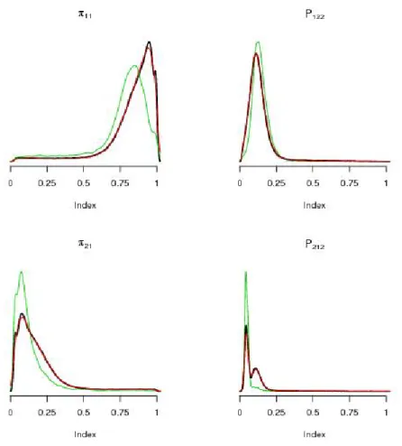
3.4.2 Posterior Density Estimation . . . 53
3.4.3 Comparison to MARCH 3.0 software . . . 56
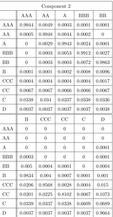
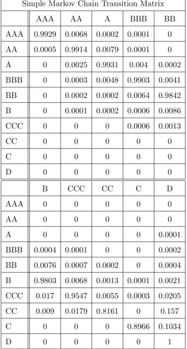
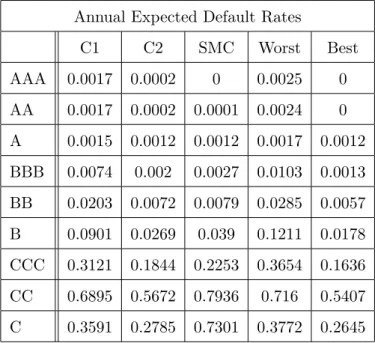
3.5 Applications to Standard and Poor’s credit rating data . . . 58
3.6 Discussion . . . 65
3.6.2 Further Research . . . 67
4 Mixtures of Markov chains 68 4.1 The continuous-time Markov chain . . . 69
4.2 General finite mixtures of continuous-time Markov chains . . . 76
4.3 Testing between 1 and 2 mixture components . . . 81
4.3.1 A parametric bootstrap procedure to test for the presence of a mixture . . . 83
4.3.2 Non-identifiability of the likelihood ratio test . . . 86
4.3.3 Divergence of the log-likelihood ratio test statistic . . . 90
4.3.4 A special case with 2 states . . . 99
5 Censored exponential mixture detection 102 5.1 An overview of the testing problem . . . 104
5.2 Testing homogeneity in censored exponential mixture models . . . . 106
5.3 Details of original proofs . . . 116
5.3.1 Proof of Lemma 5.1 . . . 122 5.3.2 Proof of Lemma 5.2 . . . 124 5.3.3 Proof of Theorem 5.3 . . . 128 5.3.4 Proof of Lemma 5.4 . . . 130 5.3.5 Proof of Lemma 5.5 . . . 132 5.3.6 Proof of Theorem 5.6 . . . 134 6 Conclusion 135
1
Introduction
In this work, we explore the theory and applications of various multi-regime mod-els involving Markov chains. Markov chains are an elegant way to model path-dependent data. We study a series of problems with non-homogeneous data and the various ways that Markov chains come into play. Non-homogeneous data can be modelled using multi-regime models, which apply a distinct set of parameters to distinct population sub-groups, referred to asregimes. Such models essentially allow for a practitioner to understand the nature (and in some cases the existence) of particular regimes within the data without the need to split the population into assumed sub-groups. Examples of problems involving non-homogeneous data include the problem of modelling business outcomes in different economic states (without explicitly using economic variables) or studying rainfall patterns as the seasons change across geographies. The problems we discuss here involve multiple regimes in two different ways and they also involve Markov chains in two different ways. Different regimes can apply to an entire population at different times, which we see in our first two problems, and different regimes can also apply to different subsections of the population over the whole observed time, which we see in our second two problems. Markov chains are involved via the estimation procedure or within models for the observed data. We first study multi-regime problems with Markov chains used in the estimation procedure. These are conducted from a Bayesian approach and we utilise the properties of Markov chains to discover and establish efficiencies in the estimation algorithms. Following this, we explore the uses of Markov chains as components of models applied to non-homogeneous data. Note that our second problem involves Markov chains in both the estima-tion procedure as well as the model. Although this work is largely focussed on addressing the theoretical issues of each problem, the motivation behind each of
that are insufficiently described through more standard procedures.
Our first problem is motivated by a simple form of non-homogeneous data. We study a single discrete time series representing quarterly driver fatality counts for the state of Victoria, Australia. Upon inspection of the data, it is clear that there are shifts in the levels of the counts over different time periods. Thus, there is a need to model the non-homogeneous dataset, allowing for multiple regimes. We apply a Bayesian Poisson change-point model to the data, using a Gibbs sampler, and note that there is no way of knowing how many iterations of the sampler will be required for a sufficient level of convergence. We derive a key property of the Markov chain involved in the Gibbs sampler procedure to estimate the parameters of a Poisson change-point model, which provides a significant insight into the nature of the convergence rate of the sampler. This enables us to have greater confidence around the model estimates and the resulting insights gained on the phenomena driving the multiple regimes in the data.
We continue with the use of Bayesian estimation algorithms for our second problem, which is motivated by the regime-switching nature of credit rating mi-gration dynamics for a homogeneous population of firms. This is a problem with more complex discrete time-series data, with multiple series of different lengths. This dataset is modelled using the double chain Markov model (DCMM), where we have a hidden Markov chain that drives the switching process between two Markov chains that drive the observed data. Similar to the first problem, we also estimate the model using a Markov chain Monte Carlo procedure and show how it can be applied to model credit rating migration data over discrete time and identify where the key regime switches occur, which aligns remarkably well with notable economic events of the past few decades in the United States. We exploit the properties of the Markov chain underlying the estimation procedure to en-hance the efficiency of the sampling algorithm. We show using simulation studies
that we are able to improve the estimation efficiency, when compared to existing estimation procedures.
The application of credit rating migration modelling is also the motivation for our third problem. However, instead of supposing that the different regimes occur over time, we look at different regimes that drive a particular proportion of the population over the whole of the finite observation window. We are thus looking at a Markov chain mixture model and focus on the problem of testing for the number of mixture components. We prove that the log-likelihood ratio test statistic, for the test between 1 and 2 Markov chain components, diverges to infinity with probability 1.
We then outline a simplified version of the model, where we only have 2 possi-ble states for each Markov chain component, one fornon-default and an absorbing state for default, and state a theorem that gives the exact limiting distribution of the log-likelihood ratio test statistic for this version of the problem. This test is equivalent to the test between 1 and 2 components in a mixture of censored ex-ponentials. We ultimately find the exact limiting distribution of the log-likelihood ratio test statistic for this challenging problem, which would allow us to test for the presence of a mixture for this class of models.
Our first problem is explored in Chapter 2, where we apply the Poisson change-point model to driver fatality counts for the state of Victoria, Australia. The different regimes arise from evolving policy settings with some causing the fatal-ities to drop significantly. We fit this model with a Bayesian approach using the Gibbs sampler, a commonly used Markov chain Monte Carlo procedure. Our sam-pler starts with initial parameter estimates that are sampled from their respective prior distributions, which are used to sample a subset of the parameters from the conditional distributions that arise from knowing the complementary subset, then conditioning on these new samples to re-sample the initial subset. This iterative
procedure continues until the resulting samples of each parameter have distribu-tions that resemble their true marginal distribudistribu-tions. If these sample distribudistribu-tions are in a steady state and have low values of the autocorrelation function at each lag k≥1 with respect to the index of the sampled chain of estimates, then we say that the algorithm has converged. Note here that the conditional distribution of future samples, conditional on the current and past samples, is only dependent on the current sample and not the samples preceding it. This is the Markov property of the Gibbs sampler. The chain is the series of samples for the full parameter vector and the state space of the chain is the corresponding combined parameter space of the model. In order to generate appropriate parameter estimates (and distributions around each), we require that the Markov chain of the Gibbs sam-pler is able to explore all possibilities in the parameter space. That is, we require that the Markov chain be ergodic. If there was an absorbing state, for example, the Markov chain would not be ergodic. This could mean that a particular Gibbs sampler may eventually sample the value that results in the absorbing state and all subsequent samples for that parameter would be the same. This would not allow the sampler to explore all areas of the parameter space but only a small section of it. Sometimes a Markov chain can be ergodic but the chance of an arbitrary chain exploring a particular part of the distribution is so low that it is barely sampled from, even after many iterations of the algorithm. In a practical setting, we require algorithms to be fast and thus need to know the rate at which the Markov chain in the Gibbs sampler has explored all areas of the parameter space sufficiently. We utilise some key results in the literature to show that if a particular sampler has certain properties, we can show that the Markov chain in the sampler is geomet-rically ergodic. That is, it explores all areas of the parameter’s sample space at a geometric rate, meaning that only a moderate amount of iterations are necessary to have a sufficiently rich sample from the parameter space to fit the model.
Key results of this chapter have been published in Fitzpatrick (2014), which was produced as a key component of this thesis with the overarching theme of multi-regime models involving Markov chains. Here, our observations derive from underlying regimes that change over time and we estimate the parameters using a procedure involving a Markov chain. Our key result is on finding a particular prop-erty of this Markov chain, geometric ergodicity, which has important implications for our estimation procedure and hence the reliability of our results.
In Chapter 3, as well as using Markov chain Monte Carlo for estimation, we explore a model that uses Markov chains to describe the data dynamics directly. We are modelling the credit rating dynamics of hundreds of financial services firms in the United States of America across a time period that spans many different economic states. We note that the rating dynamics vary widely enough to warrant a multi-regime model. Since the broader economy is often described as a cycle, with growth and contraction periods, we choose to fit two regimes and also model the switching process between these regimes with a Markov chain. This is known as the double chain Markov model (DCMM). The observed data is driven by a Markov chain at each time point; however, the particular Markov chain that drives the data is selected by a hidden Markov chain, which models the switching dynamics. We estimate all of the parameters with an efficient Bayesian algorithm to ensure that all areas of the parameter space are sufficiently explored to allow for effective convergence of the Gibbs sampler as in Chapter 2. After fitting the model to the credit rating data, we find that not only do the two regimes clearly represent good and bad credit migration dynamics but they are selected for the time periods that are well known to be the good and bad times of the United States economy. This is a remarkable finding, given that only the credit rating migration dataset was used with no economic information used a priori. It has always been a challenge for practitioners to model business dynamics, particularly
when it comes to rare events such as defaults of highly rated firms. The double chain Markov model allows for a few parameters to describe complex dynamics that can assist in understanding the credit risk taken by banks and large investment firms. When we allow for multiple regimes, we are able to estimate the dynamics that occur during times of economic stress. We know from the recent financial crisis of 2008-2009, which had truly global effects, that economic conditions can vary quite dramatically from the long-term average. Thus, we are working in an area that is in great need of further exploration. The iterative model estimation algorithms, the data, computing power, model consistency and general theory all must be explored further to extend the tools available for understanding these dynamics.
Key results of this chapter have been published in Fitzpatrick and Marchev (2013), which was produced as a key component of this thesis with the overarching theme of multi-regime models involving Markov chains. The observed data are driven by different underlying regimes, which switch between each other over time, and Markov chains are involved in a number of ways. Firstly, in a similar way to the previous chapter, the estimation is performed by running a Markov chain. Secondly, the series of regimes that are selected over time is a Markov chain, meaning that, conditional on the current regime, the regime we select for the next time point is independent to the previous regimes. Finally, the parameters of the observed model are also Markov chains. This is because the credit rating data that we study have a discrete state at each time point and the dynamics of their potential migration to other ratings in the future, given a selected regime, is only dependent on their current state.
We study a different need for multi-regime models in Chapter 4 where the different regimes apply to different subsets of the population. We continue with the motivating problem of modelling the credit rating migration dynamics of firms;
however, we look into the theory behind the test for the number of Markov chains required to satisfactorily fit a particular dataset. We explore this problem with mixtures of continuous-time Markov chains and specifically develop the theory for the test between 1 and 2 Markov chain components in the mixture. We conjecture that, similarly to Hartigan (1985), the log-likelihood ratio test statistic diverges to infinity with the sample size, contrary to the claim from Frydman (2005) that we can use standard theory to apply a chi-squared distribution with degrees of freedom equal to the difference in the number of parameters between the 1 component and 2 component mixture models. We provide evidence for our conjecture with the use of a parametric bootstrap procedure and then adapt the theory of Fukumizu (2003) to our case to definitively prove that the log-likelihood ratio test statistic does in fact diverge to infinity with the sample size. In order to develop a test for the presence of a Markov chain mixture, the next step would be to derive the limiting distribution of the log-likelihood ratio test statistic. We pursue this for a special case in the following chapter.
In Chapter 5, we focus on a simple case of the model in Chapter 4, where each Markov chain component consists of a non-default state and an absorbing default state. We derive the exact limiting distribution of the log-likelihood ratio test statistic for the test between 1 and 2 Markov chain mixture components. This test is equivalent to the test between 1 and 2 components in a censored exponential mixture problem. We show that the log-likelihood ratio test statistic is asymptotically equivalent to the square of the maximum of a Gaussian process over an interval whose length increases as the logarithm of the sample size. We prove that this Gaussian process is locally stationary so that we may utilise the extreme value theory developed in H¨usler (1990) to ultimately derive the exact limiting distribution of the log-likelihood ratio test statistic. These developments allow us to conduct a two sided test between 1 and 2 censored exponential mixture
components, which has applications beyond our original motivating example. We provide some conclusions and ideas for future research following our results.
2
Geometric ergodicity of the Gibbs sampler for
the Poisson change-point model
In order to understand the changing rates of driver fatalities over the past 20 years in the state of Victoria, Australia, we observe a discrete time series of quarterly counts between March 1989 and December 2010, shown in Figure 1. From inspec-tion, we can see that there is an initial sharp drop in the counts for each quarter, before a levelling off followed by another drop in the counts and a further levelling off. Although the more recent data is generally lower than the previous years, it does not seem to be following a linear trend, nor a gradual geometric decline. There seems to be multiple levels in the data for various time intervals but it isn’t entirely obvious where these levels are. If the count data seemed to have one level of propensity, then we could fit a simple Poisson model. However, due to the multiple levels of counts, it is appropriate to apply a Poisson change-point model to the data. This will allow us to estimate where the change-points are, where we shift to a new regime and what the fatality rates are in each regime.
Poisson change-point models are used for modelling inhomogeneous time-series of count data. There are a number of methods available for estimating the param-eters in these models using iterative techniques such as Markov chain Monte Carlo (MCMC). Many of these techniques share the common problem that there does not seem to be a definitive way of knowing the number of iterations required to obtain sufficient convergence. In this chapter, we show that the Gibbs sampler of the Poisson change-point model is geometrically ergodic. Establishing geometric ergodicity is crucial from a practical point of view as it implies the existence of a Markov chain central limit theorem, which can be used to obtain standard error estimates. We prove that the transition kernel is a trace-class operator, which implies geometric ergodicity of the sampler (see Khare and Hobert (2011) for
de-Fatal Crashes in Victoria
Time
Count
1990
1995
2000
2005
2010
60
120
180
Figure 1: The count of driver fatalities in Victoria for each quarter between March 1989 and December 2010. Source: TAC (2011)
tails). We then examine the application of the sampler to a Poisson change-point model for quarterly driver fatality counts for the state of Victoria, Australia.
2.1
Introduction
Under the Poisson change-point model, we observe a non-homogeneous sequence ofT independent Poisson random variablesX1, . . . , XT. More specifically, we
con-sider the case when the rate λ changes from λ1 to λ2 at an unknown point τ1,
then fromλ2 toλ3 at a later unknown point τ2, and so on, until the rate changes
to λK, where it remains for the observation periods τK + 1 to T. This model
has been widely studied (see Carlin et al. (1992) and Raftery and Akman (1986), among others). Each of these models have a fixed K, which means the number of change-points is known a priori. The Bayesian Poisson change-point model
studied in Raftery and Akman (1986) assumed conjugate priors and has a single change-point at an unknown time. The model is applied to a well known data set consisting of intervals between coal-mining disasters given by Jarrett (1979). Car-lin et al. (1992) present a general approach to hierarchical Bayesian change-point models, including a version of the Poisson change-point model that we apply to our data, and describes a Gibbs sampler procedure in great detail. Although Carlin et al. (1992) acknowledge the need to derive the number of iterations and sampler replications required for sufficient convergence, the convergence of the algorithm is concluded through inspection of the postetior distribution for the parameters after applying up to 50 iterations and 100 replications. Further understanding of the properties of convergence of the Gibbs sampler for the Poisson change-point model will allow for a more precise number of iterations and replications to be directly derived.
Here, we use a Poisson change-point model for detecting the shifts and levels of quarterly driver fatality counts for the state of Victoria, Australia. Within this application, the timing and size of the shifts in the dynamics of the data provide insight into the effectiveness of particular government policies in reducing the number of road fatalities.
In this study of non-homogeneous count data for driver fatalities in Victoria, we utilise the results from Khare and Hobert (2011) to show a theoretical result on the convergence of the Gibbs sampler for estimating the model parameters that is of great importance to practitioners. In cases where these models are utilised for providing objective evidence to influence future policy-making, we must have confidence that the iterative algorithm for estimating the model parameters has converged. It is an interesting approach to providing statistical evidence of shifts in outcomes. Traditionally, a hypothesis would be set that assumes a particular effect is or is not present and this hypothesis is tested as to whether we should adopt the
defined alternative. This essentially requires us to know what the alternatives are. For example testing whether data could be derived from a particular model (such as the standard normal distribution), we would produce a test statistic that has a particular distribution under the null hypothesis and infer with a particular level of confidence whether we should reject this hypothesis in favour of a more general alternative. However, with the class of models discussed here, we are only assuming a model form and then using the data to allow us to discover the potential causes for shifts in the rates of driver fatalities. This differs to us needing to guess the potential causes first then test for whether we should guess again. If the results from this more exploratory approach align with independent prior ideas as to what could be driving the data, our understanding can be further verified.
In Section 2.2, we outline the model specification and introduce some notation. We then discuss the estimation of the model parameters in Section 2.3. The main result is presented in Section 2.4 where we show that the Gibbs sampler is geometrically ergodic. This is a specific application of the results of Khare and Hobert (2011) to our model chosen here due to its practical significance. These theoretical results are used in practice in Section 2.5, where we apply the model to quarterly driver fatality counts for the state of Victoria, Australia. Our main interest is in estimating the non-constant fatality rate λ and the change-points τ = (τ1, . . . , τK) by obtaining a sample from their posterior distributions.
We are interested in estimating both the timing of the change-points as well as the size of the shift in fatality rates. The significant shifts in the driver fatality counts, which are thankfully being reduced over time, align with some key policy implementations and public campaigns, providing evidence for their impact. A comparison of the fatality rates in each regime provides a measurement of their effectiveness, despite the natural variation in the data from year to year. We then discuss some conclusions and potential avenues for future research.
2.2
Model specification
For the application of modelling the quarterly driver fatality counts, we are pre-sented with a time series of count data. That is, a series of 0 < T < ∞ positive integers Y1, Y2, . . . , YT representing the number of driver fatalities in each
quar-ter. Upon inspection of Figure 1, we see that these numbers vary over the series within a reasonably controlled range and we see immediately that the earlier data points tend to have higher counts than the later data points. We are modelling these data in an exploratory fashion, to understand the features of the data, any patterns that emerge and the resulting insights this can give us about what to expect with future data points given relationships with causal factors that are not directly captured in the data (such as road safety regulations, number of cars, size and density of the population, types of vehicles on the roads, quality of the roads, quality of the drivers, weather and natural disasters etc.). Note that it is impossible to discern exactly what the causes are but we can show evidence that supports or challenges a particular claim. We could look to capture other infor-mation that may be related to the data and find a statistical relationship such as fitting a generalised linear model of sorts; however, this requires access to many other sources of data for the same time period and region involved. Given that our analysis is largely exploratory, we would be required to gather much more data than an eventual model as we should keep an open mind as to what may have the strongest relationship with our dependent variables. Alternatively, we can find patterns in our count data and use these patterns to point us in the right direction what could be causing these patterns to emerge. This approach is key. It starts with the data and we are guided to a greater understanding of what drives it.
Let us refer to the probability of a driver fatality within a particular time period with a particular risk level. Focussing again on the actual counts, we note that although the counts are greater for the earlier years than the later years, there
does not seem to be a steady decline. In fact, there seems to be a single step down in the counts and a levelling out before another step down. This multi-level effect points to a shift in risk levels that are constant for a certain period before shifting to a new level for the next period and so on. If we modelled all of the data with a regular Poisson model, we would not have a good idea of the level of risk at each time point but rather a view of the average risk over the entire observable period. From inspection, we see that a constant level of risk is certainly not appropriate. Poisson models may work to describe the count data but we must allow for the shift in the risk levels.
We thus consider the Poisson change-point model, where
Yi|λ, τ ind. ∼ Po(λ1) for i= 1, . . . , τ1; Po(λ2) for i=τ1+ 1, . . . , τ2; .. . Po(λK) for i=τK−1+ 1, . . . , τK; Po(λK+1) fori=τK+ 1, . . . , T . λi|β, τ ind. ∼ G(ai, βi), i= 1, . . . , K + 1 βi|τ ind. ∼ IG(ci, ρi), i= 1, . . . , K + 1 (1)
0 < K ≤ T −1 is a known constant and τ1, . . . , τK are distributed as the order
statistics from a random sample of sizeK taken without replacement from the set {1,2, . . . , T −1}.
Here X ∼G(a, b) implies that X follows the gamma density
fX(x) = x
a−1
baΓ(a)e
−x
b, x > 0 and X ∼ IG(c, ρ) implies that X follows the inverse gamma density fX(x) = ρcxc+11Γ(c)e
−1
ρx, x > 0.
The particular form of this model is consistent with the literature. In fact, if we fix K = 1, then we have the Poisson change-point model that was studied in Carlin et al. (1992). It is also constructed for a Bayesian approach. Given the
data, there is no way for us to produce consistent maximum likelihood estimates as we do not know when the shifts in λ take place. If we knew when the shifts were (or guessed) then fitting the model with a frequentist approach would be trivial. However, with this approach we allow the timing of the shifts to vary, thus allowing the data to provide guidance as to where these could be. We may also analyse the posterior distribution of the parameters, given their prior distributions and the information provided by the data, which can give us a greater idea of our level of certainty with each of the parameters and the potential that there may be something quite different going on. The choice of prior distributions is consistent with the sort of data that we are analysing (count data that occurs where there are multiple experiments with a low risk of a particular outcome being experienced). These distributions are also conjugate prior distributions. That is, they retain their form in the posterior distribution after being combined with the data likelihood distribution.
We will firstly explore some theoretical properties of this general model before applying it specifically to our practical task at hand. This is the first time that this particular dataset has been analysed in this way, so our findings will be of use to policy makers seeking to further understand the drivers of the data. We also extend the theory to further our understanding of the rate of convergence of the Gibbs sampler for this model, which gives us some guidance as to the running time required for the iterative algorithm to fit the model before we can analyse the parameters and extract practical insights.
2.3
Estimation of the model parameters
Recall that our main interest is in estimating the vector λ and the change-points τ = (τ1, . . . , τK) by obtaining a sample from their posterior distributions. From
(1) we obtain the joint density f(y,λ,β,τ) = T1−1 K τ1 Y h=1 λyh 1 e−λ1 yh! K Y i=2 τi Y j=τi−1+1 λyj i e−λi yj! T Y k=τK+1 λyk Ke −λK yk! K+1 Y l=1 λal−1 l βal l Γ(al) e−λlβl K+1 Y m=1 1 ρcm m βmcm+1Γ(cm) e−ρmβm1 . (2)
Then, the complete posterior density is
f(λ,β,τ|y)∝λ Pτ1 i=1yi+a1−1 1 K Y k=2 λ Pτk i=τk−1+1yi+ak+1−1 k+1 λ PT i=τK+1yi+a2−1 K+1 × e−λ1(τ1+β1 1)QK k=2 n e−λk(τk−τk−1+βk1 )o e−λK+1(T−τK−1+βK1 +1)QK+1 k=1 n e−ρkβk1 o βa1+c1+1 1 β a2+c2+1 2 .
The desired sample will be obtained by running a two-stage Gibbs sampler that iterates between
f(λ|β,τ,y) and f(β,τ|λ,y),
where the sequence of β’s will be simply ignored.
From (2), it is clear that conditional on β,τ,y, the parameters λ1, . . . , λK+1
are independent with
λ1|β,τ,y∼G τ1 X i=1 yi+a1, β1 τ1β1+ 1 ! ; λk|β,τ,y∼G τk X i=τk−1+1 yi+ak, βk (τk−τk−1)βk+ 1 for k = 2, . . . , K; λK+1|β, τ,y∼G T X i=τK+1 yi+aK+1, βK+1 (T −τK)βK+1+ 1 ! . (3)
and τ are independent with βk|λ,y∼IG ak+ck, ρk ρkλk+ 1 for k= 1, . . . , K+ 1; f(τ|λ,y) = f(y|τ,λ) PT−K−1 τ10=1 PK i=2 PT−K−1+i τi0=τi0−1+1f(y|τ 0,λ). (4) Remarks:
1. Note that we intentionally chose the parametrization of the gamma and inverse gamma densities so that equations (3) and (4) agree perfectly with the complete conditional distributions derived in Carlin et al. (1992).
2. It is possible to integrate out the βvariables from the posterior density. For example, in the case of one change-point, we see that
f(λ, τ|y)∝ λ Pτ i=1yi+a1−1 1 λ PT i=τ+1yi+a2−1 2 e−λ1τ e−λ2(T−τ) (ρ1λ1+ 1)a1+c1(ρ2λ2+ 1)a2+c2 .
However, the above density, although available in closed form (apart from a normalizing constant), is not easy to draw from. Moreover, the introduction of more than one change point makes sampling from f(λ,τ|y) even harder, whereas with our approach the algorithm is essentially the same.
2.4
Geometric ergodicity of the Gibbs sampler
In this section we prove that the Gibbs sampler, originally described by Geman and Geman (1984), applied to the Poisson change-point model, specified in the previous section, is geometrically ergodic. A geometrically ergodic Gibbs sampler converges to its target distribution at a geometric rate. We do this by using the results in Khare and Hobert (2011) about data augmentation (DA) algorithms which are trace-class. DA algorithms involve the introduction of unobserved or
latent variables to sampling or iterative optimisation procedures. Stochastic DA algorithms constructed for posterior sampling can take the form of a two-block Gibbs sampler, such as the one used for our model.
Definition 2.1. If a DA algorithm based on a joint density f(x, y) satisfies
Z Θ Kmo(θ|θ)dθ = Z Y Z X fX|Y(x|y)fY|X(y|x)µ(dx)ν(dy)<∞, (5)
then the Markov operator,Kmo, associated with the chain is atrace-classoperator.
Here, Θ = X × Y and also fX|Y(x|y) and fY|X(y|x) are the densities for the
parameter subsets X and Y with measures µand ν respectively.
Furthermore, if Kmo is a trace-class operator then it is compact and its norm kKmok<1, so by Roberts and Rosenthal (1997), the corresponding Markov chain
must be geometrically ergodic. Further details about trace-class operators can be found, for example, in Conway (1990).
We can prove geometric ergodicity of the Gibbs sampler for our model via the following theorem.
Theorem 2.2. For the Poisson change-point model (1), the two conditional den-sities (3) and (4) satisfy
T−K−1 X τ1=1 K X i=2 T−K−1+i X τi=τi−1+1 Z RK++1 Z RK++1 f(λ|β,τ,y)f(β,τ|λ,y)dβdλ<∞. (6)
Therefore, the Gibbs sampler for the Poisson change-point model (1) is geo-metrically ergodic.
We can see from (5) that (6) implies that the Markov operator associated with the Gibbs sampler for the Poisson change-point model (1) is a trace-class operator.
We can then use the results of Roberts and Rosenthal (1997) to see that the Gibbs sampler for (1) is geometrically ergodic.
Proof. From (3) and (4) we can see that the left hand side becomes
T−K−1 X τ1=1 K X i=2 T−K−1+i X τi=τi−1+1 Z ∞ 0 . . . Z ∞ 0 f(λ1|β1,τ,y). . . f(λK+1|βK+1,τ,y)f(β1|λ1) × . . . f(βK+1|λK+1)f(τ|λ,y)dβ1. . . dβK+1dλ1. . . dλK+1. Note that f(τ∗|λ,y) = f(y|τ ∗,λ) PT−K−1 τ1=1 PK i=2 PT−K−1+i τi=τi−1+1f(y|τ,λ)
≤1 for all possible τ∗,
which implies that the left hand side of the expression in the theorem is bounded above by T−K−1 X τ1=1 K X i=2 T−K−1+i X τi=τi−1+1 Z ∞ 0 . . . Z ∞ 0 f(λ1|β1,τ,y) . . . f(λK+1|βK+1,τ,y) × f(β1|λ1) . . . f(βK+1|λK+1)dβ1. . . dβK+1dλ1. . . dλK+1 = T−K−1 X τ1=1 K X i=2 T−K−1+i X τi=τi−1+1 Z ∞ 0 Z ∞ 0 f(λ1|β1,τ,y)f(β1|λ1)dβ1dλ1 × . . . × Z ∞ 0 Z ∞ 0 f(λK+1|βK+1,τ,y)f(βK+1|λK+1)dβK+1dλK+1 .
Thus, since T is finite and since f(λk|βk,τ,y) and f(βk|λk) are distributed simi-larly for all k= 1, . . . , K+ 1, then it will suffice to prove that
Z ∞
0
Z ∞
0
Note also that lettingM(τ1) =τ1,M(τK+1) =T−τK, andM(τi) =τi−τi−1 for
i = 2, . . . , K, and letting N(τ1) = Pτj1=1yj, N(τK+1) = PTj=τK+1yj, and N(τi) =
Pτi j=τi−1+1yj for i= 2, . . . , K, we have f(λi|y,τ, bi) ∼ G ai+N(τi), bi biM(τi) + 1 f(bi|λi) ∼ IG ai+ci, ρi ρiλi+ 1
where ai, ci, and ρi are known positive constants, for i = 1, . . . , K + 1. Thus,
taking the model specification into account, for any general τ ∈ {1, . . . , T −1} and N(τ) = Pτ
i=1yi, we are required to prove
Z ∞ 0 Z ∞ 0 λa+N(τ)−1e−λ(τ+1b) (bτb+1)a+N(τ)Γ(a+N(τ)) e−1b(λ+ 1 ρ) (ρλρ+1)a+cΓ(a+c)ba+c+1dbdλ <∞. (8)
We will do this by bounding the left hand side by integrable functions. We will bound the left and right tails of each of thebandλsupports by a different function and show that the result is still finite.
LHS = Z ∞ 0 Z ∞ 0 I1dbdλ = Z ∞ 0 Z ∞ 0 λa+N(τ)−1(λ+ 1 ρ) a+ce−λ(τ+2b) Γ(2a+N(τ) +c+ 1)(bτb+2)2a+N(τ)+c+1dλ × " Γ(2a+N(τ) +c+ 1)(bτb+2)2a+N(τ)+c+1e−1b( 1 ρ) (bτb+1)a+N(τ)Γ(a+c)Γ(a+N(τ))ba+c+1 # db < Z ∞ 0 Z M 0 I1dλdb+ Z ∞ 0 Z ∞ M λ2a+N(τ)+ce−λ(τ+2 b) Γ(2a+N(τ) +c+ 1)( b bτ+2) 2a+N(τ)+c+1dλ × " Q1(bτb+2)2a+N(τ)+c+1e −1 b( 1 ρ) (bτb+1)a+N(τ)ba+c+1 # db
xa+c+1 ∀ ρ, a, c >0 and x > M. So now, we have LHS < Z ∞ 0 Z M 0 I1dλdb+Q1 Z ∞ 0 (bτ + 1)a+N(τ)e−1b( 1 ρ) (bτ + 2)2a+N(τ)+c+1ba+c+1db < Z ∞ 0 Z M 0 I1dλdb+Q1 Z ∞ 0 e−1b( 1 ρ) (bτ + 2)a+c+1db < Z ∞ 0 Z M 0 I1dλdb+Q1ρa+cΓ(a+c) Z ∞ 0 e−1b( 1 ρ) ba+c+1ρa+cΓ(a+c)db = Z ∞ 0 Z M 0 I1dλdb+Q2
where Q2 =Q1ρa+cΓ(a+c). Thus we can now focus on the first term, so
LHS <Q2+ Z M 0 Z ∞ 0 (bτ + 1)a+N(τ)e−1b(2λ+ 1 ρ) b2a+N(τ)+c+1Γ(2a+N(τ) +c)( ρ 2ρλ+1) 2a+N(τ)+cdb × " Γ(2a+N(τ) +c)(2ρλρ+1)2a+N(τ)+cλa+N(τ)−1e−λτ (ρλρ+1)a+cΓ(a+c)Γ(a+N(τ)) # dλ
and since there existsN >0 such that (bτ+1)a+N(τ) < bda+N(τ)+1e∀b, τ, a, N(τ)> 0 and b > N, <Q2+ Z M 0 Z N 0 I1dbdλ + Z M 0 E[bda+N(τ)+1e]Γ(2a+N(τ) +c)( ρ 2ρλ+1) 2a+N(τ)+cλa+N(τ)−1e−λτ (ρλρ+1)a+cΓ(a+c)Γ(a+N(τ)) dλ <Q2+ Z M 0 Z N 0 I1dbdλ + Z M 0 Γ(2a+N(τ) +c− da+N(τ) + 1e) (2ρλρ+1)da+N(τ)+1e (2ρλρ+1)a+N(τ)λa+N(τ)−1e−λτ Γ(a+c)Γ(a+N(τ)) dλ <Q2+ Z M 0 Z N 0 I1dbdλ + Z M 0 Γ(2a+N(τ) +c− da+N(τ) + 1e) Γ(a+c)Γ(a+N(τ)) 2λ+1 ρ da+N(τ)e e−λτdλ =Q3+ Z M 0 Z N 0 I1dbdλ where Q3 = Q2+MΓ(2a+N(τ)+c −da+N(τ)+1e) Γ(a+c)Γ(a+N(τ)) sup0<λ<M(2λ+1ρ)da+N(τ)ee−λτ, and
under the condition that 2a+c−dae 6= 1,0,−1,−2, . . ., which is not very restrictive. Therefore, the last thing to prove is that
A= Z M 0 Z N 0 I1dbdλ <∞. (9)
For this, we note that the mode of an IG(α, β) distribution is β(α1+1) and the mode of a G(α, β) distribution is α−β1. Thus, we have
A < Z M 0 Z N 0 (a+N(τ)−1)b bτ + 1 ρλ+ 1 ρ(a+c+ 1)dbdλ = Z M 0 Z N 0 I2dbdλ
and since ∂I2 ∂b = (a+N(τ)−1)(ρλ+ 1) ρ(a+c+ 1)(bτ + 1)2 >0 for all 0≤b ≤N, we have A < N Z M 0 (a+N(τ)−1)(ρλ+ 1) ρ(a+c+ 1)(N τ+ 1)2 dλ. Also, ∂ ∂λ (a+N(τ)−1)(ρλ+ 1) ρ(a+c+ 1)(N τ+ 1)2 = (a+N(τ)−1)ρ ρ(a+c+ 1)(N τ + 1)2 >0∀ 0≤λ≤M, so we have A < M N(a+N(τ)−1)(M ρ+ 1) ρ(a+c+ 1)(N τ + 1)2 <∞. Therefore, Z Θ Kmo(θ|θ)dθ <∞ as required.
2.5
Applications to Victorian driver fatality count data
A popular application of the Poisson change-point model is in the assessment of the effectiveness of government policies. We analyse count data for the number of fatal crashes in each calendar quarter, recorded in the state of Victoria, Australia. The data is from the Australian Government - Department of Infrastructure and Transport, TAC (2011). This particular time series is of interest due to the factpast twenty years, despite an increase in the number of drivers over the same period. It is important to assess the nature of the reductions, whether it is a steady downward trend or whether there are sudden drops due to various effective policies or other discrete influences.
Our data set consists ofT = 88 quarterly observations, ranging from the March quarter of 1989 to the December quarter of 2010. We fit the Poisson change-point model from (1), with K = 2 change-points, to the data. The constant hyperparameters are set with a1 = 170, a2 = 120, a3 = 80, c1 =c2 =c3 = 1, and
ρ1 =ρ2 =ρ3 = 1, so that the sampled rate parametersλi are more likely to begin
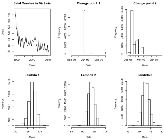
with values that roughly mirror the values in Figure 1. The algorithm runs for 100,000 iterations, after a burn-in period of 10,000 iterations. The results are as shown in Figure 2.
The estimated change-points are after the June quarter of 1990 and the March quarter of 2002. The first change-point was a major drop that followed the imple-mentation of the Road Safety Act (1986), which governs road use and deals with licensing and road related offences in Victoria. This also lead to the establishment of the Transport Accident Commission (TAC), which is the statuatory insurer of third-party personal liability. In 1989 there was also a federal Ten Point Plan to reduce the number of deaths on Australian roads. The TAC have also launched successful TV advertising campaigns in Victoria throughout the 1990’s and early 2000’s. In 2000, the National Road Safety Strategy 2001-2010 was developed, with a target of a 40 per cent reduction in the population rate of road fatalities from 9.3 to 5.6 per 100,000. The Strategy was supported by a series of two-year action plans. The introduction of this targeted focus on road fatality reduction coincided with the second change-point seen in the data.
It is difficult to discern exactly what causes the change-points. However, it is evident that significant shifts in the rate of road fatalities in Victoria have been
Fatal Crashes in Victoria Time Count 1990 2000 2010 60 80 100 120 140 160 180 Change point 1 Date Fre qu en cy 0 20000 40000 60000 80000
Dec-89 Jun-90 Dec-90
Change point 2 Date Fre qu en cy 0 10000 20000 30000 40000 50000
Dec-01 Mar-03 Jun-04
Lambda 1 Rate Fre qu en cy 130 150 170 0 5000 15000 25000 35000 Lambda 2 Rate Fre qu en cy 85 90 95 100 0 5000 10000 15000 20000 25000 Lambda 3 Rate Fre qu en cy 65 70 75 80 0 5000 10000 15000 20000 25000
Figure 2: Crash statistics data with Poisson change-point model parameters
observed and assuming that the behaviour of the general population is consistent over time, it is likely that the introduction and implementation of these major policy introductions have lead to a significant reduction in road fatality rates. The model parameter estimates allow us to measure the difference in rates. From the ratios of the posterior estimates of λ2/λ1 and λ3/λ2, we see that the first
change-point lead to a drop in road fatalities of between 36 and 45 per cent and the second change-point lead to a drop in road fatalities of between 18 and 26 per cent, at the 95 per cent confidence level. This form of objective feedback to the effectiveness of major policy decisions is vital to continued high levels of governance.
2.6
Conclusions
On a practical level, we have seen how the Poisson change-point model can be estimated for modelling road fatalities, where there are various policies and laws in place at different times. The model clearly shows shifts in the count levels towards a lowered rate of fatalities, despite a rise in the population of drivers. Given the validity of the datapoints, we can conclude that the level of fatalities has significantly reduced over the past 20 years. It would be of interest to see if these results held true for other states and territories around Australia, which could help identify the cause of the decline in fatalities. For example, if the downward shifts occur around the same time, it could indicate the cause of the decline in fatalities was due to a federal intervention. On a theoretical level, the results in this chapter imply that the Gibbs sampler for the Poisson change-point model will converge at a geometric rate. Thus, given a specific convergence level, the minimum number of iterations required can be calculated. Although we have identified a key quality of the convergence rate of the sampler, the calculation of the specific rate of convergence is left for further research. It would also be of interest to see if the bounding technique of section 2.4 can be used to prove geometric ergodicity of MCMC algorithms for other models.
3
Efficient Bayesian estimation of the
multivari-ate double chain Markov model
Key results of this chapter have been published in Fitzpatrick and Marchev (2013), which was produced as a key component of this thesis with the overarching theme of multi-regime models involving Markov chains. The observed data are driven by different underlying regimes, which switch between each other over time, and Markov chains are involved in a number of ways. Firstly, in a similar way to the previous chapter, the estimation procedure is a Markov chain. Secondly, the series of regimes that are selected over time is a Markov chain, meaning that, conditional on the current regime, the regime we select for the next time point is independent to the previous regimes. Finally, the parameters of the observed model are also Markov chains. This is because the credit rating data that we study have a discrete state at each time point and the dynamics of their potential migration to other ratings in the future, given a selected regime, is only dependent on their current state.
The double chain Markov model (DCMM) is used to model an observable pro-cess Y ={Yt}Tt=1 as a Markov chain with transition matrix,Pxt, dependent on the value of an unobservable (hidden) Markov chain {Xt}Tt=1. We present and justify
an efficient algorithm for sampling from the posterior distribution associated with the DCMM, when the observable processY consists of independent vectors of (pos-sibly) different lengths. Convergence of the Gibbs sampler, used to simulate the posterior density, is improved by adding a random permutation step. Simulation studies are included to illustrate the method. The problem that motivated our model is presented at the end. It is an application to real data, consisting of the credit rating dynamics of a portfolio of financial companies where the (unobserved) hidden process is the state of the broader economy.
3.1
Introduction
LetY be a set ofJ elements. For convenience we will denote them with the first J
positive integers; i.e.,Y ={1, . . . , J}. Consider a stochastic process{Yt}T
t=0, where
each Yt takes values in Y for t = 0, . . . , T. Dependence among such Yt’s, taking
values in a finite state space, can be modeled by Markov chains. For example, the first order simple Markov chain model can be described as follows:
P (Y1, . . . , YT)>= (y1, y2, . . . , yT)>|Y0 =y0, θ = T Y t=1 θyt−1yt,
where θ is a J ×J transition matrix such that θij = P(Yt = j|Yt−1 = i, θ) for
t = 1, . . . , T, i, j = 1, . . . J and the elements in each row of θ sum to 1. In other words, regardless of any external factors that may affect the observations, given the state yt of the random variable at the current time, it migrates with the same multinomial distribution of probabilities (θyt1, . . . , θytJ) to the other possible states. A more rigorous definition of Markov chains in a general state space can be found in Meyn and Tweedie (1993).
There have been different extensions to the simple Markov chain model that have emerged in the literature. One of the most important has been the Hid-den Markov model (HMM) which was first presented in the late 1960’s in Baum and Petrie (1966) and can be regarded as a Markov chain observed with noise. More precisely, a HMM is a stochastic process {(Yt, Xt)}T
t=0, where {Xt}Tt=0 is a
hidden Markov chain (i.e. unobservable), and {Yt}Tt=0 is a sequence of
(observ-able) independent random variables such that the distribution of Yt depends on Xt, t= 0, . . . , T. An excellent book on inference in HMM’s is Capp´e et al. (2005).
Various applications, in areas such as meteorology, biotechnology, finance and speech recognition, have motivated the exploration of the properties of HMM’s.
For example, Churchill (1989) uses HMM’s to study the sequences of bases on a DNA molecule and Hughes et al. (1999) study the relationship between observed rainfall occurrence and broad scale atmospheric circulation patterns via HMM’s. These models have also been popular in their application to credit modeling in recent years. Studies such as Giampieri et al. (2005), and Korolkiewicz and Elliott (2008) use HMM’s to model credit rating dynamics, by making the assumption that the observed ratings are not dependent upon previous observed ratings but rather on the hidden variables, representing the effects of the broader economy. A good summary of the bibliography on HMM’s can be found in Capp´e (2001).
Since the model we consider in this chapter is a version of a HMM, we now describe the HMM in more detail. Assume that the hidden process{Xt}Tt=0evolves
independently of {Yt}T
t=0 and is a Markov chain with first-order transition matrix
Π of dimension a×a and initial state distribution Π0 := (π01, . . . , π0a)>. Assume
further that at each time point t= 0, . . . , T, depending on the value of the hidden process xt, there are a finite number, a, of possible distributions of the random
variable Yt that takes values in the set Y. We write the mass function of Yt as P(Yt=yt|Xt =xt,Θ) = θxt,yt, where Θ = {θk,l, k = 1, . . . , a, l∈ Y}, are unknown parameters. That is, letting θ={Π0,Π,Θ}, the HMM can be described as
P(y0, . . . , yT, x0, . . . , xT|θ) = P(y0, . . . , yT|x0, . . . , xT, θ)P(x0, . . . , xT|θ) = P(x0|Π0)P(y0|θx0) T Y t=1 [P(yt|xt,Θ)P(xt|xt−1,Π)] = π0x0θx0,y0 T Y t=1 θxt,ytπxt−1,xt.
These models work well for modeling the heterogeneity of the observed process over time. However, they do not incorporate any direct dependence between ob-servations. The logical extension is to allow the hidden Markov process to select
one of a finite number of Markov chains to drive the observed process at each time point. This sort of model is known as the double chain Markov model (DCMM) and was first formally presented in Berchtold (1999). It is basically designed for modeling non-homogeneous time series. If a time series can be decomposed into a finite mixture of Markov chains, then the DCMM can be applied to describe the switching process between these chains. This idea is not entirely new. The first extension was to combine the HMM with an autoregressive model for the observed process in Poritz (1982) and later in Kenny et al. (1990). Then Wellekens (1987) and Paliwal (1993) presented a model, similar to the DCMM for both the continu-ous case of the HMM and the discrete case respectively. Berchtold (1999) differed from Paliwal (1993) with a more rigorous derivation of the forward-backward and Viterbi algorithms involved in the model estimation and also by interpreting the relation between observed outputs of the model as a non-stationary Markov chain. There have been extensions to the DCMM presented in Berchtold (1999), in-creasing the order of the Markov chains as in Eisenkopf (2008). However, this leads to an explosion in the number of parameters. There exist alternatives to modeling higher order dependence in Markov chains, such as in the mixture transition distri-bution (MTD) model presented in Raftery (1985), which presents the conditional probability of the current state as a linear combination of contributions from each of a fixed number of past states. An iterative algorithm for the estimation of these models was described in Berchtold (2002). The DCMM was extended in Eisenkopf (2008) using the theory of MTD’s in Berchtold (2002) to show that the DCMM can handle higher order relationships among the hidden states as well as the observed outputs.
There are alternative generalizations of the HMM, which also take into account the heterogeneity of mixture models over time. In Lanchantin et al. (2008), the triplet Markov chain (TMC) model is presented, which can be viewed as an
al-ternative generalization of HMM’s that is slightly different to the DCMM, where the non-stationary distribution of the hidden Markov chain was modelled by an auxiliary process governing the switching of the transition matrix over time (in the DCMM, the hidden process is time-homogeneous). There are several explo-rations of the TMC, such as in Pieczynski and Desbouvries (2005) and Pieczynski (2007). Finally, we point the interested reader to Kirshner (2005), where there is a detailed description of all levels of generalization from HMM’s to models such as the DCMM, where there are direct relationships between the observed states, to non-homogeneous hidden Markov models with autoregressive observed states, similar to the TMC.
The computational estimation of the DCMM is explored in Berchtold (1999). Due to the structure of the DCMM, there is no direct formula to compute the log-likelihood. The problem is solved using an iterative procedure known as the forward-backward algorithm. The estimation of the model parameters is tradi-tionally obtained by an expectation-maximisation (EM) algorithm known in the speech recognition literature as the Baum-Welch algorithm. Finally, the optimal sequence of hidden states is computed using another iterative procedure called the Viterbi algorithm presented in Forney (1973).
This chapter is focused specifically on multivariate time series data, which is especially relevant in the context of modeling vectors of observations of different lengths for each time point, such as in credit portfolio applications. The estima-tion of the hidden states, the model parameters and the hidden Markov process parameters is from a Bayesian perspective and is carried out using an efficient extension of the techniques presented in Chib (1996). In order to improve the convergence speed of the Gibbs sampler used to simulate the posterior density, we employ the random permutation sampler presented in Fr¨uhwirth-Schnatter (2001). During each iteration of the sampling process, the hidden states are sampled from
their joint distribution, given the current parameter estimates and the observed data. Then, we randomly permute the current labelling of the states of the hidden process. This permutation of the labels is justified and is shown to be optimal us-ing the recent results of Hobert and Marchev (2008). After obtainus-ing the MCMC sample, a post-processing algorithm from Stephens (2000), as presented in Boys and Henderson (2002), is utilised to find the most suitable permutation of the labels at each run of the sampler so that a consistent form of the model results, without the non-identifiability arising from label switching.
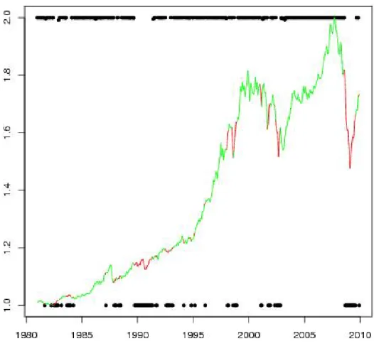
Our work was motivated by the lack of appropriate models in the context of credit portfolio modelling. In this setup the hidden Markov process represents the effects of the broader economy and governs the particular regime driving the transitions of credit ratings in a large portfolio of firms for each time point. We apply our model on a dataset comprised of monthly Standard and Poor’s (S&P) credit rating transitions for a portfolio of globally sourced financial institutions and insurance companies from the 1st of January 1981 to the 1st of January 2010. The estimated switching behavior of the hidden Markov regimes selected for each time point bear remarkable similarities to the behaviour of the global economy over the last three decades, as explained in Section 5.
The chapter is organised as follows. In Section 3.2 we specify the model and introduce the notation and background to the theory of DCMM’s. In Section 3.3, we estimate the model parameters from a Bayesian perspective, using an efficient Data Augmentation (DA) algorithm in combination with the post-processing al-gorithms of Stephens (2000) and Boys and Henderson (2002). Section 3.4 displays the results of the model when applied to simulated data. In Section 3.5 we apply our model on real data from Standard and Poor’s. Finally, Section 3.6 provides conclusions and ideas for further research in this area.
3.2
Model specification
In this section, we describe our multivariate Bayesian DCMM and its parameters and derive the density function of the complete data set, consisting of both hidden and observed variables.
Consider data of n random variables observed discretely over time, each of potentially different lengths. That is, for each i = 1, . . . , n, we observe a vector, (yi,ui, . . . yi,mi)
>, where ui < mi. Define
u0 := min
1≤i≤n{ui}, andM := max1≤i≤n{mi}
and note that the times ui and mi may vary over the entire observation period
fromu0, . . . , M with the only restriction thatmi−ui ≥1, i= 1, . . . , n.
Assume that for each i = 1, . . . , n and each time point t = ui, . . . , mi, the
random variable Yi,t ∈ Y, where Y = {1, . . . , J}, and is modelled as dependent
upon the value at the previous time point, yi,(t−1), as well as on a hidden state,
xt, for that time point. We assume that the hidden process X = {Xt}Mt=u0 is
a Markov chain with first-order transition matrix Π of dimension a×a, where
πgh = P(Xt =h|Xt−1 = g) for g, h = 1, . . . , a and t =u0 + 1, . . . , M. We let the
first hidden state Xu0 be selected from a multinomial distribution with vector of
probabilities r = (r1, . . . , ra)>. We also assume that the observable process is a
Markov chain witha possible transition matricesP1, . . . , Pa, each of orderJ ×J,
such that for a given hidden statext, the elements of the transition matrixPxt are
pxt,jk = P(Yi,t =k|Yi,(t−1) =j, Xt=xt),
for i= 1, . . . , n, t=ui+ 1, . . . , mi.
initial observed state yi,ui and the number of consecutive time-points that it was observed mi −ui + 1 as fixed so all inference is conditional on those values. We denote the collection of all parameters in our model by θ and observe that θ ∈ Θ, where Θ is the d-dimensional hypercube with d equal to the number of free parameters in the model, since all parameters are probabilities between 0 and 1.
Conditional on X, each of the random variables are modelled independently of each other. For each i= 1, . . . , n, if we define yi, := (yi,(ui+1), . . . , yi,mi)
>, then
we consider the following hierarchical Bayesian model:
P(yi,|yi,ui,x, θ) = P(yi,(ui+1)|yi,ui, xui+1)× · · · × ×P(yi,mi|yi,(mi−1), xmi) P(x|θ) = P(xu0)P(xu0+1|xu0)× · · · × ×P(xM|xM−1) P(θ) = P(r)P(Π)P(P1). . .P(Pa), (10)
where, similarly to Chib (1996), the priors on r, Π, P1, . . . , Pa are Dirichlet as
follows: r ∼D(α01, . . . , α0a) (πi1, . . . , πia) ind ∼ D(αi1, . . . , αia), i= 1, . . . , a (p1,l1, . . . , p1,lJ) ind ∼ D(α1,l1, . . . , α1,lJ), l= 1, . . . , J .. . (pa,l1, . . . , pa,lJ) ind ∼ D(αa,l1, . . . , αa,lJ), l= 1, . . . , J,
and theα’s are given constants. More details on how priors are chosen for HMM’s can be found in Subsection 13.1.2 of Capp´e et al. (2005).
Then the model for Y := (Y1,, . . . ,Yn,) is P(y|y0,x, θ) = n Y i=1 P(yi,|yi,ui,x, θ), (11) where y0 := (y1,u1, . . . , yn,un)
> and P(x|θ) and P(θ) are as specified in (10).
From equation (10) the joint mass function of Yi, and X givenyi,ui and θ is:
P(yi,,x|yi,ui, θ) = rxu0πxu0xu0+1. . . πxuixui+1pxui+1,yi,uiyi,(ui+1) × · · · ×πxmi−1xmipxmi,yi,(mi−1)yi,mi. . . πxM−1xM = " a Y l=1 rI{xu0}(l) l # M Y t=u0+1 a Y g=1 a Y h=1 πI{(xt−1,xt)}(g,h) gh × " mi Y t=ui+1 a Y l=1 J Y j=1 J Y k=1 pI{(yi,(t−1),yi,t,xt)}(j,k,l) l,jk # , (12)
where IA(x) is the usual indicator function of a set A.
Next, we utilise the fact that the random vectors Yi, for i = 1, . . . , n are
independent, conditional on the hidden process X, when deriving the joint mass function of all random variables Y and X:
P(y,x|y0, θ) = " a Y l=1 rI{xu0}(l) l # " M Y t=u0+1 a Y g=1 a Y h=1 πI{(xt−1,xt)}(g,h) gh # × " n Y i=1 mi Y t=ui+1 a Y l=1 J Y j=1 J Y k=1 pI{(yi,(t−1),yi,t,xt)}(j,k,l) l,jk # . (13)
We are interested in exploring the posterior density f(θ|y) := ff(y(y,θ)), where
f(y, θ) and f(y) are defined from (13) and (10) as
f(y, θ) = X
x∈Xm
and f(y) =RΘf(y, θ)dθ withXm being them-tuple product of the set {1, . . . , a}
with itself. Here, m = M −u0 + 1. Of course, given the nature of P(y,x|y0, θ)
in (13) and the summation in (14), direct calculation of f(θ|y) is impossible; however, as explained in the next section, it is possible to construct an efficient MCMC algorithm to obtain approximate draws from it.
3.3
Estimation of the model parameters
The target density f(θ|y), as defined in the previous section, is not available in closed form, but can be presented as the θ-marginal density of f(θ,x|y), where
f(θ,x|y) = f(y,x|y0,θ)P(θ)
f(y) . Therefore, we will employ the data augmentation (DA)
algorithm of Tanner and Wong (1987) to obtain approximate draws from it. Thus, we run a two-stage Gibbs sampler that alternates between sampling from
P(x|y, θ) := f(θ,x|y)
f(θ|y) (15)
and
P(θ|x,y) := f(θ,x|y)
f(x|y) , (16)
wheref(x|y) is the x-marginal density of f(θ,x|y). The exact forms of (15) and (16) are derived in the next two subsections.
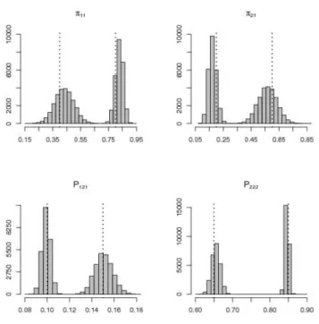
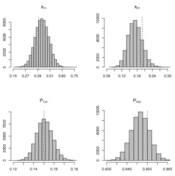
It is well-known that in Bayesian mixture models, there is the so called problem of “label switching”, which means that the target posterior density is multi-modal and the sampler can easily get stuck in one of the modes (or explore the modes ir-regularly). We remedy this issue by performing an additional step, which randomly permutes the labels after sampling from (15). This random permutation step was introduced in Fr¨uhwirth-Schnatter (2001) and further analyzed in Hobert et al. (2011) as being a special case of the general scheme for improvement of DA algo-rithms, presented in Hobert and Marchev (2008). What we will show in Subsection
3.3.3 is that this extra step is also optimal in the sense of Hobert and Marchev (2008), as being constructed via a group action on Xm with the appropriate Haar
measure.
Finally, the parameters θ are estimated as posterior means, calculated from the output of the modified DA algorithm, after a post-processing step is applied (as detailed in Subsection 3.3.4).
3.3.1 Sampling from P(x|y, θ)
Chib (1996) developed a method for simulating the hidden states x, given a par-ticular i∈ {1, . . . , n} and a single vector of observed data, yi,. We will generalise this algorithm to a set of multiple vectors y1,, . . . ,yn, of different lengths.
For u0 < t < M define x−t:= (xu0, . . . , xt) xt:= (xt, . . . , xM) y,t := [ i:ui<t
(yi,ui, . . . , yi,min{t,mi})
yt:= [
i:t<mi
(yi,max{t+1,ui}, . . . , yi,mi)
y(t) := {yi,t} for all i∈ {1, . . . , n} with ui ≤t≤mi,
and note that the first, third and fifth definitions are also valid for t=M. The following lemma is used to derive P(x|y, θ):
Lemma 3.1. For t=u0, . . . , M −1 we have
Proof. For all t=u0, . . . , M −1 we have
LHS = P(xt+1|xt,y,t, θ)
= P(y,t|xt, xt+1, θ)P(xt+1|xt, θ) P(y,t|xt, θ)
= P(xt+1|xt, θ)
since, by the definition of the model in (10), the observable data up to any such time
t is not dependent upon the unobservable data at time t+ 1 and only dependent on the unobservable data up to timet and θ. Then,
P(xt+1|xt, θ) = P(xt+1|xt,Π)
since, by the definition of the model in (10), the unobservable data is driven by a hidden Markov chain with transition matrix Π that is not dependent upon the other parameters.
Our main result about sampling from P(x|y, θ) follows.
Theorem 3.2. For data of independent vectors {Yi,}ni=1 the joint distribution,
P(x,y, θ), of the hidden data, the observed data and the parameters is given by
P(x,y, θ)≡P(x−M|y,M, θ) ∝ P(xM|y,M−1, θ)f y(M)|y,M−1, θxM × M−1 Y t=u0+1 P(xt+1|xt,Π)P(xt|y,t−1, θ)f y(t)|y,t−1, θxt ×P(xu0+1|xu0,Π)P(xu0|r) with P(xt|y,t−1, θ) = a X l=1 P(xt|xt−1 =l,Π)P(xt−1 =l|y,t−1, θ).
and the remaining components are from the model specified in equations (10) and (11).
Proof. The joint mass function of the hidden states, given the parameters and the observed data as vectors at each time point is
P(x−M|y,M, θ) = P(xM|y,M, θ)×. . . ×P(xt|y,M,xt+1, θ)· · · ×P(xu0|y,M,xu0+1, θ).
The “typical term” can be written as
P(xt|y,M,x t+1, θ) = P(x t|y,t,y t+1,xt+1, θ) = P(x t+1,yt+1|y ,t, xt, θ)P(xt|y,t, θ) P(xt+1,yt+1|y ,t, θ) = P(xt|y,t, θ) P(xt+1,xt+2,yt+1|y,t, xt, θ) P(xt+1,yt+1|y ,t, θ) = P(xt|y,t, θ)P(xt+1|xt,y,t, θ) P(xt+2,yt+1|y ,t, xt, xt+1, θ) P(xt+1,yt+1|y ,t, θ) = P(xt|y,t, θ)P(xt+1|xt,Π) P(xt+2,yt+1|y,t, xt, xt+1, θ) P(xt+1,yt+1|y ,t, θ) by Lemma 3.1. Now, P(xt+2,yt+1|y,t,xt,xt+1,θ) P(xt+1,yt+1|y ,t,θ)
depends only on xt+1, and is therefore
independent ofxt and thus can become the normalising constant. That is,
P(xt|y,M,xt+1, θ)∝P(xt|y,t, θ)P(xt+1|xt,Π). (17)
We continue, in more detail, to show
P(xt|y,t, θ) = P(xt|y,t−1,y(t), θ)
= P(xt|y,t−1, θ)P(y(t)|xt,y,t−1, θ) P(y(t)|y,t−1, θ)
∝P(xt|y,t−1, θ)f(y(t)|y,t−1, θx ).
By the law of total probability and Lemma 3.1, we have P(xt|y,t−1, θ) = a X l=1 P(xt|xt−1 =l,y,t−1, θ)P(xt−1 =l|y,t−1, θ) = a X l=1 P(xt|xt−1 =l,Π)P(xt−1 =l|y,t−1, θ)
and consequently from (17) and (18),
P(xt|y,M,xt+1, θ) ∝ P(xt+1|xt,Π) " a X l=1 P(xt|xt−1 =l,Π)P(xt−1 =l|y,t−1, θ) # ×f y(t)|y,t−1, θxt .
This is initialized at t =u0 by setting P(x0|y,M, θ) = P(xu0|r) to be the same as
the Dirichlet prior on D(α01, . . . , α0a).
3.3.2 Sampling from P(θ|x,y) Define n0,l :=I{xu0}(l), l = 1, . . . , a, ngh := M X t=u0+1 I{(xt−1,xt)}(g, h), g, h= 1, . . . , a, nl,jk := n X i=1 mi X t=ui+1 I{(yi,(t−1),yi,t,xt)}(j, k, l), for j, k = 1, . . . , J, l= 1, . . . , a.
Then from Equation (13), combined with the Dirichlet priors, it can be seen thatP(θ|x,y) can be simulated separately and independently for r,Π and all the
P’s as follows: r|x,y ∼ D(α0,1+n0,1, . . . , α0,a+n0,a) π11, . . . , π1a|x,y ∼ D(α11+n11, . . . , α1a+n1a) .. . πa1, . . . , πaa|x,y ∼ D(αa1+na1, . . . , αaa+naa).
For the parameters for the observed process in each regimel = 1, . . . , a, this yields
pl,11, . . . , pl,1J|x,y ∼ D(αl,11+nl,11, . . . , αl,1J +nl,1J)
.. .
pl,J1, . . . , pl,J J|x,y ∼ D(αl,J1+nl,J1, . . . , αl,J J +nl,J J).
3.3.3 Extra permutation step
To improve the convergence properties of the DA algorithm at each iteration of the Gibbs sampler, we conduct a random permutation of the labels, as detailed in Fr¨uhwirth-Schnatter (2001). Here we show that this extra step is justified and is optimal in the sense of Hobert and Marchev (2008). What they denote by Y is our Xm and what they denote by Xis our Θ.
From (14) it can be seen that the posterior of interest, f(θ|y), is theθ-marginal density of f(x, θ|y); i.e., f(θ|y) = P
x∈Xmf(x, θ|y) =
R
Xmf(x, θ|y)µ(dx), where
µ is the counting measure on Xm. Clearly, this form of the target density allows
for construction of the optimal Haar PX-DA algorithm, as defined in Hobert and Marchev (2008). Here we will show that the random permutation sampler of Fr¨uhwirth-Schnatter (2001) is a specific case of the Haar PX-DA algorithm.
itself:
Xm ={(x
1, . . . , xm) :xi ∈ X, i= 1, . . . , m}
={1, . . . , a}m
wherem =M−u0+1. Notice thatX, as any other discrete space, is a particularly
simple topological space, equipped with the discrete metric
d(x,x˜) = 0, x= ˜x 1, x6= ˜x , ∀ x,x˜ ∈ Xm.
Any discrete space with discrete metric is separable and locally compact and all subsets are open (and closed). In addition, we need to define a group action on Xm. Let G be the symmetric group on the set X; i.e.,
G:=SX :={permutations of (1, . . . , a)},
again equipped with the discrete metric. Finally, define the group action on Xm
as
F(g,x) =gx= (g(x1), . . . , g(xm)),
which just permutes the values of the labels. (For example, if J = 3, x = (3,2,1,1) ∈ X4, and g = (2,3,1), then gx = (1,3,2,2).) Then for the identity
permutation e, we have ex= (x1, . . . , xm) = x, and for any two permutations g1
and g2, (g1g2)x=g1(g2x). As a multiplier we take χ(g) = 1, ∀ g ∈SX. Then,