Short-Term Load Forecasting using Artificial Neural Network Techniques

SHORT-TERM LOAD

FORECASTING USING ARTIFICIAL

NEURAL NETWORK TECHNIQUES

A THESIS SUBMITTED IN PARTIAL FULFILLMENT OF THE

REQUIREMENTS FOR THE DEGREE OF

BACHELOR OF TECHNOLOGY

In

Electrical Engineering

By

MANOJ KUMAR

ROLL NO. 10502053

Department of Electrical Engineering

National Institute of Technology

LOAD FORECASTING USING

ARTIFICIAL NEURAL NETWORK

TECHNIQUES

A THESIS SUBMITTED IN PARTIAL FULFILLMENT OF THE

REQUIREMENTS FOR THE DEGREE OF

BACHELOR OF TECHNOLOGY

In

Electrical Engineering

By

MANOJ KUMAR

ROLL NO. 10502053

Under the Guidance of

PROF. K.R. SUBHASHINI

Department of Electrical Engineering

National Institute of Technology

National Institute of Technology

Rourkela

CERTIFICATE

This is to certify that the thesis entitled

“Load Forecasting using Artificial

Neural Network Techniques”

submitted by

Manoj Kumar (10502053),

in

the partial fulfillment of the requirement for the degree of

Bachelor of

Technology

in

Electrical Engineering

, National Institute of Technology,

Rourkela, is an authentic work carried out by them under my supervision.

To the best of my knowledge the matter embodied in the thesis has not been submitted to any other university/institute for the award of any degree or diploma.

Date: (Prof K. R

.

Dept of Electrical Engineering

National Institute of Technology

Rourkela-769008

ACKNOWLEDGEMENT

I wish to express my profound sense of deepest gratitude to my guide and

motivator Prof. K. R. Subhashini, Electrical Engineering Department, National

Institute of Technology, Rourkela for her valuable guidance, sympathy and

co-operation and finally help for providing necessary facilities and sources during

the entire period of this project.

I wish to convey my sincere gratitude to all the faculties of Electrical

Engineering Department who have enlightened me during my studies. The

facilities and co-operation received from the technical staff of Electrical Engg.

Dept. is thankfully acknowledged.

Last, but not least, I would like to thank the authors of various research articles

and book that referred to.

Manoj Kumar

(10502053)

CONTENTS

Abstract ………. vi

List of Figures ………. vii

List of Graphs ………. vii

List of Tables ………. vii

Abbreviations Used ………. viii

Chapter 1 Introduction to ANN ………. 1 - 7 1.1What is Neural Network? ………. 2

1.2Why do we use ANN? ………. 3

1.3History of Neural Networks ………. 4

1.4Benefits of Neural Network ………. 5

1.5Biological model of a neuron ………. 5

Chapter 2 Structure of ANN ………. 8 - 13 2.1 Mathematical model of a neuron ………... 9

2.2 Network architectures ………. 10

2.3 Learning processes ………. 13

Chapter 3 Back -propagation algorithm ………. 14 - 19 3.1 Introduction ………. 15

3.2 Learning process ………. 16

3.3 Flowchart ………. 19

Chapter 4 Function Approximation ………. 20 - 24 4.1 What is Function Approximation? …………. 21

4.2 Approximation of Linear Function ……….. 22

4.3 Approximation of Sinc Function ..……… 23

Chapter 5 Load Forecasting using ANN ………. 25 - 38 5.1 Load Forecasting ………. 26

5.2 Approach ………. 28

5.3 ANN Model ………. 29

5.4 Preprocessing of training data …………... 31

5.5 Program ………. 32

5.6 Results ………. 34

Conclusion ………. 39

ABSTRACT

Artificial Neural Network (ANN) Method is applied to fore cast the short-term load for a large power system. The load has two distinct patterns: weekday and weekend-day patterns. The weekend-day pattern includes Saturdays, Sunday and Monday loads. A nonlinear load model is proposed and several structures of ANN for short term forecasting are tested. Inputs to the ANN are past loads and the output of the ANN is the load forecast for a given day. The network with one or two hidden layers is tested with various combinations of neurons, and the results are compared in terms of forecasting error. The neural network, when grouped into different load patterns, gives good load forecast.

This project presents a study of short-term hourly load forecasting using Artificial Neural Networks (ANNs). To demonstrate the effectiveness of the proposed approach, publicly available data from the Australian national electricity market (NEMMCO) web site has been taken to forecast the hourly load for the Victorian power system. We predicted the hourly load demand for a full week with a high degree of accuracy. Historical load data of 2006 obtained from the NEMMCO web site was divided into several where half of them are used for training and the other half is used for testing the ANN.

The inputs used were the hourly load demand for the full day (24 hours) for the state and the daily temperature, humidity and wind speeds of two major cities. The outputs obtained were the predicted hourly load demand for the next day. The neural network used has 3 layers: an input, a hidden, and an output layer. The number of inputs was 37 while the number of hidden layer neurons was varied for different performance of the network. The output layer has 24 neurons.

We trained the network over 6 weeks. An absolute mean error of 2.64% was achieved when the trained network was tested on one week‟s data.

LIST OF FIGURES

Fig 1.1 Block Diagram of a Human Nervous System. ………. 5

Fig 1.2 Schematic Diagram of Biological Neuron. ………. 7

Fig 2.1 Model of an ANN. ………. 9

Fig 2.2 Single-layer Feedforward Network. ………. 10

Fig 2.3 Multi-layer Feedforward Network ………. 11

Fig 2.4 Recurrent Network. ………. 12

Fig 3.1 Three Layer Neural Network with 2 I/P and a single O/P ………. 16

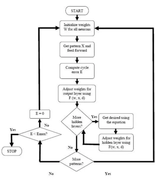
Fig 3.2 Flowchart showing working of Back Propagation Algorithm ………. 19

Fig 5.1 Input Output schematic for Load Forecasting ………. 29

Fig 5.2 Network Structure for Load Forecating ………. 30

LIST OF GRAPHS Graph 4.1 Error Squared graph of Linear Function ………. 22

Graph 4.2 Response Matching of Linear Function ………. 23

Graph 4.3 Error Square graph of Sinc Function ………. 24

Graph 4.4 Response matching of inc Function ………. 24

Graph 5.1 Actual v/ Predicted Load for Sunday ………. 34

Graph 5.2 Actual v/ Predicted Load for Monday ………. 35

Graph 5.3 Actual v/ Predicted Load for Tuesday ………. 35

Graph 5.4 Actual v/ Predicted Load for Wednesday ………. 36

Graph 5.5 Actual v/ Predicted Load for Thursday ………. 36

Graph 5.6 Actual v/ Predicted Load for Friday ………. 37

Graph 5.7 Actual v/ Predicted Load for Saturday ………. 37

Graph 5.8 Error Square Graph for Load Forecasting ………. 38

LIST OF TABLES Table 5.1 Absolute Mean Errors (AME) for the predicted week ………. 38

ABREVIATIONS USED

ANN Artificial Neural Network

MLP Multi-layer Perceptron

BPA Back Propagation Algorithm

PCA Principal Component Analysis

NEM National Electricity Market

Chapter

1

ARTIFICIAL NEURAL NETWORKS

What are ANNs?

Why do we use ANN?

History of ANN

Benefits of ANN

Biological Model

WHAT ARE ANNs?

Work on artificial neural network has been motivated right from its inception by the recognition that the human brain computes in an entirely different way from the conventional digital computer. The brain is a highly complex, nonlinear and parallel information processing system. It has the capability to organize its structural constituents, known as neurons, so as to perform certain computations many times faster than the fastest digital computer in existence today. The brain routinely accomplishes perceptual recognition tasks, e.g. recognizing a familiar face embedded in an unfamiliar scene, in approximately 100-200 ms, whereas tasks of much lesser complexity may take days on a conventional computer.

A neural network is a machine that is designed to model the way in which the brain performs a particular task. The network is implemented by using electronic components or is simulated in software on a digital computer. A neural network is a massively parallel distributed processor made up of simple processing units, which has a natural propensity for storing experimental knowledge and making it available for use. It resembles the brain in two respects:

1. Knowledge is acquired by the network from its environment through a learning process.

2. Interneuron connection strengths, known as synaptic weights, are used to store the acquired knowledge.

The procedure used to perform the learning process is called a learning algorithm, the function of which is to modify the synaptic weights of the network in an orderly fashion to attain a desired design objective.

WHY DO WE USE NEURAL NETWORKS?

Neural networks, with their remarkable ability to derive meaning from complicated or imprecise data, can be used to extract patterns and detect trends that are too complex to be noticed by either humans or other computer techniques. A trained neural network can be thought of as an "expert" in the category of information it has been given to analyse. This expert can then be used to provide projections given new situations of interest and answer "what if" questions.

Other advantages include:

1. Adaptive learning: An ability to learn how to do tasks based on the data given for training or initial experience.

2. Self-Organization: An ANN can create its own organization or representation of the information it receives during learning time.

3. Real Time Operation: ANN computations may be carried out in parallel, and special hardware devices are being designed and manufactured which take advantage of this capability.

Fault Tolerance via Redundant Information Coding: Partial destruction of a network leads to the corresponding degradation of performance. However, some network capabilities may be retained even with major network damage.

HISTORY OF ANN

Neural network simulations appear to be a recent development. However, this field was established before the advent of computers, and has survived at least one major setback in several eras.

Many important advances have been boosted by the use of inexpensive computer emulations. Following an initial period of enthusiasm, the field survived a period of frustration and disrepute. During this period when funding and professional support was minimal, important advances were made by relatively few researchers. These pioneers were able to develop convincing technology which surpassed the limitations identified by Minsky and Papert. Minsky and Papert, published a book (in 1969) in which they summed up a general feeling of frustration (against neural networks) among researchers, and was thus accepted by most without further analysis. Currently, the neural network field enjoys a resurgence of interest and a corresponding increase in funding.

The first artificial neuron was produced in 1943 by the neurophysiologist Warren McCulloch and the logician Walter Pits. But the technology available at that time did not allow them to do too much.

BENEFITS OF ANN

1. They are extremely powerful computational devices. 2. Massive parallelism makes them very efficient.

3. They can learn and generalize from training data – so there is no need for enormous feats of programming.

3. They are particularly fault tolerant – this is equivalent to the “graceful degradation” found in biological systems.

4. They are very noise tolerant – so they can cope with situations where normal symbolic systems would have difficulty.

5. In principle, they can do anything a symbolic/logic system can do, and more

.

BIOLOGICAL MODEL

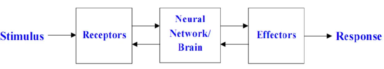
The human nervous system can be broken down into three stages that may be represented as follows:

The receptors collect information from the environment. The effectors generate interactions with the environment e.g. activate muscles. The flow of information/activation is represented by arrows.

There is a hierarchy of interwoven levels of organisation:

1. Molecules and Ions

2. Synapses 3. Neuronal microcircuits 4. dendritic trees 5. Neurons 6. Local circuits 7. Inter-regional circuits

8. Central nervous system

There are approximately 10 billion neurons in the human cortex. Each biological neuron is connected to several thousands of other neurons. The typical operating speed of biological neurons is measured in milliseconds.

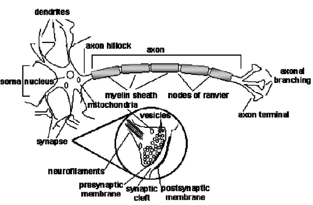
The majority of neurons encode their activations or outputs as a series of brief electrical pulses. The neuron‟s cell body processes the incoming activations and converts the into output activations. The neurons nucleus contains the genetic material in the form of DNA. This exists in most types of cells. Dendrites are fibres which emanate from the cell body and provide the receptive zones that receive activation from other neurons. Axons are

fibres acting as transmission lines that send activation to other neurons. The junctions that allow signal transmission between axons and dendrites are called synapses. The process of transmission is by diffusion of chemicals called neurotransmitters across the synaptic cleft.

Chapter

2

STRUCTURE OF ANN

Mathematical Model of a Neuron

Network Architecture

Learning Process

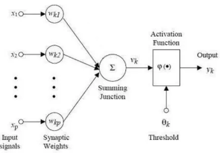
MATHEMATICAL MODEL OF A NEURON

A neuron is an information processing unit that is fundamental to the operation of a neural network. The three basic elements of the neuron model are:

1. A set of weights, each of which is characterized by a strength of its own. A signal xj

connected to neuron k is multiplied by the weight wkj. The weight of an artificial

neuron may lie in a range that includes negative as well as positive values.

2. An adder for summing the input signals, weighted by the respective weights of the neuron.

3. An activation function for limiting the amplitude of the output of a neuron. It is also referred to as squashing function which squashes the amplitude range of the output signal to some finite value.

vk =

and

yk = φ(vk + θk) (2.2)

NETWORK ARCHITECTURES

There are three fundamental different classes of network architectures [5]:

1) Single-layer Feedforward Networks

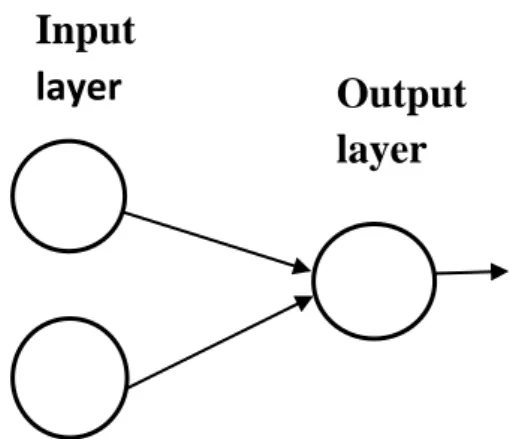
In a layered neural network the neurons are organized in the form of layers. In the simplest form of a layered network, we have an input layer of source nodes that projects onto an output layer of neurons, but not vice versa. This network is strictly a Feedforward type. In single-layer network, there is only one input and one output layer. Input layer is not counted as a layer since no mathematical calculations take place at this layer.

Fig 2.2 Single-layer Feedforward Network

Input

layer

_Output

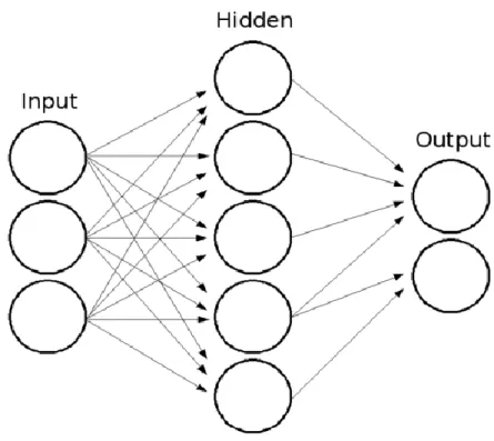
2) Multilayer Feedforward Networks

The second class of a Feedforward neural network distinguishes itself by the presence of one or more hidden layers, whose computational nodes are correspondingly called hidden neurons. The function of hidden neuron is to intervene between the external input and the network output in some useful manner. By adding more hidden layers, the network is enabled to extract higher order statistics. The input signal is applied to the neurons in the second layer. The output signal of second layer is used as inputs to the third layer, and so on for the rest of the network.

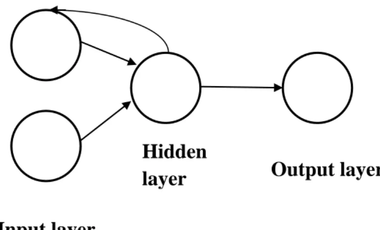
3) Recurrent networks

A recurrent neural network has at least one feedback loop. A recurrent network may consist of a single layer of neurons with each neuron feeding its output signal back to the inputs of all the other neurons. Self-feedback refers to a situation where the output of a neuron is fed back into its own input. The presence of feedback loops has a profound impact on the learning capability of the network and on its performance.

Fig 2.4 Recurrent Network

Input layer

Hidden

LEARNING PROCESSES

By learning rule we mean a procedure for modifying the weights and biases of a network. The purpose of learning rule is to train the network to perform some task. They fall into three broad categories:

1. Supervised learning

The learning rule is provided with a set of training data of proper network behavior. As the inputs are applied to the network, the network outputs are compared to the targets. The learning rule is then used to adjust the weights and biases of the network in order to move the network outputs closer to the targets.

2. Reinforcement learning

It is similar to supervised learning, except that, instead of being provided with the correct output for each network input, the algorithm is only given a grade. The grade is a measure of the network performance over some sequence of inputs.

3. Unsupervised learning

The weights and biases are modified in response to network inputs only. There are no target outputs available. Most of these algorithms perform some kind of clustering operation. They learn to categorize the input patterns into a finite number of classes.

Chapter

3

BACK PROPAGATION ALGORITHM

Introduction

Learning Process

Flowchart

INTRODUCTION

Multiple layer perceptrons have been applied successfully to solve some difficult diverse problems by training them in a supervised manner with a highly popular algorithm known as the error back-propagation algorithm. This algorithm is based on the error-correction learning rule. It may be viewed as a generalization of an equally popular adaptive filtering algorithm- the least mean square (LMS) algorithm.

Error back-propagation learning consists of two passes through the different layers of the network: a forward pass and a backward pass. In the forward pass, an input vector is applied to the nodes of the network, and its effect propagates through the network layer by layer. Finally, a set of outputs is produced as the actual response of the network. During the forward pass the weights of the networks are all fixed. During the backward pass, the weights are all adjusted in accordance with an error correction rule. The actual response of the network is subtracted from a desired response to produce an error signal. This error signal is then propagated backward through the network, against the direction of synaptic connections. The weights are adjusted to make the actual response of the network move closer to the desired response.

A multilayer perceptron has three distinctive characteristics:

1. The model of each neuron in the network includes a nonlinear activation function. The sigmoid function is commonly used which is defined by the logistic function: y = (3.1)

The presence of nonlinearities is important because otherwise the input- output relation of the network could be reduced to that of single layer perceptron.

2. The network contains one or more layers of hidden neurons that are not part of the input or output of the network. These hidden neurons enable the network to learn complex tasks.

3. The network exhibits a high degree of connectivity. A change in the connectivity of the network requires a change in the population of their weights.

LEARNING PROCESS

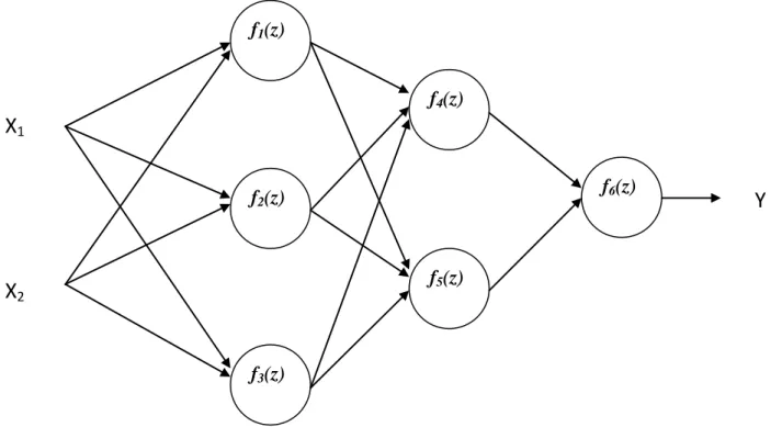
To illustrate the process a three layer neural network with two inputs and one output,which is shown in the picture below, is used.

Fig 3.1 Three layer neural network with two inputs and single output

f1(z) f2(z) f6(z) f5(z) f4(z) f3(z)

X

X

Y

Signal z is adder output signal, and y = f(z) is output signal of nonlinear element. Signal y is also output signal of neuron. The training data set consists of input signals (x1 and x2 )

assigned with corresponding target (desired output) y’. The network training is an iterative process. In each iteration weights coefficients of nodes are modified using new data from training data set. Symbols wmn represent weights of connections between output of neuron m

and input of neuron n in the next layer. Symbols yn represents output signal of neuron n.

y1 = f1(w11 x1 + w21 x2) (3.3) y2 = f2(w12 x1 + w22 x2) (3.4) y3 = f3(w13 x1 + w23 x2) (3.5) y4 = f4(w14 y1 + w24 y2 + w34 y3) (3.6) y5 = f5(w15 y1 + w25 y2 + w35 y3) (3.7) y6 = f6(w46 y4 + w56 y5) (3.8)

The desired output value (the target), which is found in training data set. The difference is called error signal δ of output layer neuron.

δ = y‟ – y (3.9)

δ4 = w46 δ (3.10)

δ5 = w56 δ (3.11)

δ3 = w34 δ4+ w35 δ5 (3.12)

δ

= w

δ

+ w

δ

When the error signal for each neuron is computed, the weights coefficients of

each neuron input node may be modified. In formulas below

df(z)/dz

represents

derivative of neuron activation function.

The correction wij(n) applied to the weight connecting neuron j to neuron i is defined by the

delta rule:

Weight correction = learning rate parameter*local gradient*i/p signal of neuron i

Δwij(n) = η . δi(n) . yj(n) (3.15)

The local gradient δi(n) depends on whether neuron i is an output node or a hidden node:

1. If neuron i is an output node, δi(n) equals the product of the derivative dfi(z)/dz and

the error signal ei(n), both of which are associated with neuron i.

2. If neuron j is a hidden node, δi(n) equals the product of the associated derivative

dfi(z)/dz and the weighted sum of the δs computed for the neurons in the next hidden

FLOW CHART

Chapter

4

FUNCTION APPROXIMATION

What is Function Approximation?

Approximation of a Linear Function

Approximation of a Sinc Function

WHAT IS FUNCTION APPROXIMATION?

Function approximation takes examples from a desired function (e.g., a value function) and attempts to generalize from them to construct an approximation of the entire function. Function approximation is an instance of supervised learning, the primary topic studied in machine learning, artificial neural networks, pattern recognition, and statistical curve fitting. In principle, any of the methods studied in these fields can be used in reinforcement learning.

The need for function approximations arises in many branches of applied mathematics, and computer science in particular. In general, a function approximation problem asks us to select a function among a well-defined class that closely matches ("approximates") a target function in a task-specific way.

One can distinguish two major classes of function approximation problems: First, for known target functions approximation theory is the branch of numerical analysis that investigates how certain known functions (for example, special functions) can be approximated by a specific class of functions (for example, polynomials or rational functions) that often have desirable properties (inexpensive computation, continuity, integral and limit values, etc.).

Second, the target function, call it g, may be unknown; instead of an explicit formula, only a set of points of the form (x, g(x)) is provided. Depending on the structure of the domain and codomain of g, several techniques for approximating g may be applicable. For example, if g

APPROXIMATION OF A LINEAR FUNCTION

The linear function taken was:

Y = 2X1 + X2 (4.1)

The network used was a Multi-layer Perceptron (MLP) network with a single hidden layer consisting of 6 neurons. The activation function for the hidden layer was “tan-sigmoid” while that of the output layer was “pure-linear”. We used a learning rate of 0.01.

The results obtained are shown below:

Graph 4.2 Response Matching of Linear Function

APPROXIMATION OF A SINC FUNCTION

The sinc function is defined by:

Sinc x = Sin(π x)/π x (4.2)

The network used was a Multi-layer Perceptron (MLP) network with a single hidden layer consisting of 11 neurons. The activation function for the hidden layer was “log-sigmoid” while that of the output layer was “pure-linear”. We used a learning rate of 0.069

The results obtained are shown below:

Graph 4.3 Error Square graph of Sinc Function.

Chapter

5

LOAD FORECASTING USING ANN

Load Forecasting

Approach

ANN Model

Preprocessing of Training Data

Program

Results

LOAD FORECASTING

There is a growing tendency towards unbundling the electricity system. This is continually confronting the different sectors of the industry (generation, transmission, and distribution) with increasing demand on planning management and operations of the network. The operation and planning of a power utility company requires an adequate model for electric power load forecasting. Load forecasting plays a key role in helping an electric utility to make important decisions on power, load switching, voltage control, network reconfiguration, and infrastructure development.

Electric load forecasting is the process used to forecast future electric load, given historical load and weather information and current and forecasted weather information. In the past few decades, several models have been developed to forecast electric load more accurately. Load forecasting can be divided into three major categories:

1. Long-term electric load forecasting, used to supply electric utility company

management with prediction of future needs for expansion, equipment purchases, or staff hiring

2. Medium-term forecasting, used for the purpose of scheduling fuel supplies and

unit maintenance

3. Short-term forecasting, used to supply necessary information for the system

Short-term power load forecasting is used to provide utility company management with future information about electric load demand in order to assist them in running more economical and reliable day-to-day operations. The power load during the year followed the same the daily and weekly periods of electric load, which represents the daily and weekly cycles of human activities and behavior patterns, with some cyclical and random changes.

The significance of space cooling on the electric load is very obvious during the summertime. When the temperature increases, the demand for electricity increases. On the other hand, during the wintertime the reverse relationship between temperature and electric demand exists because of the need for space heating. When the temperature decreases, the load demand for electricity increases. [7]

APPROACH

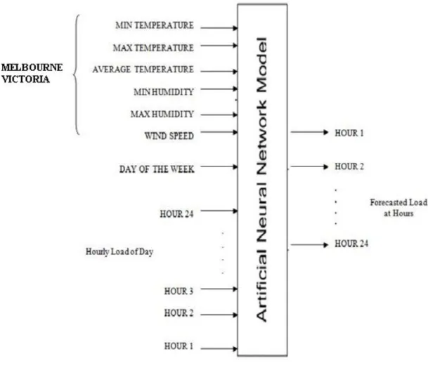
A broad spectrum of factors affect the system‟s load level such as trend effects, cyclic-time effects, and weather effects, random effects like human activities, load management and thunderstorms. Thus the load profile is dynamic in nature with temporal, seasonal and annual variations. In our project we developed a system that predicted 24 hour at a time load

demand. As inputs we took the past 24 load and the day of the week. Melbourne was chosen for Victorian region and used the daily temperature, humidity and wind speed as input parameters. The city chosen was the major city in Victoria and as such gave sufficient representation to the change in weather parameter across the state.

The inputs were fed into our Artificial Neural Network (ANN) and after sufficient training were used to predict the load demand for the next week. A schematic model of our system is shown in Fig 5.1.

The inputs given are:

1. Hourly load demand for the full day. 2. Day of the week.

3. Min/Max/ Average daily temperature (Melbourne). 4. Min/Max daily Humidity (Melbourne).

5. Daily wind speed (Melbourne).

And the output obtained was the predicted hourly load demand for the next day. The flow chart is shown below.

Fig 5.1 Input-Output Schematic for Load Forecasting.

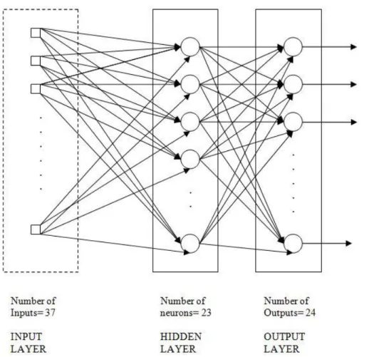
ANN Model

For our Neural Network model we used a Multi Layer Perceptron (MLP) network with a single hidden layer. The number of neurons in the hidden layer was varied between 17 and 23 before finally being set at 23 neurons. The activation function used in the hidden layer neuron was „Tan-sigmoid‟. The number of output neurons was 24 using „Pure linear‟ activation function. To set the learning rate we ran the network with a large number of different learning rates before settling on 0.07 which gave us the best results.

The ANN was implemented using MATLAB 7. The training algorithm „Traingdx‟ was used which is an adaptive learning algorithm using the epoch method of training. The number of epochs while training was set at 50,000 by which point the network was sufficiently trained.

Pre-Processing of Training Data

The data employed for training and testing the neural network were obtained from the NEMMCO website for the period June-July 2006. Due to wrong measurements and other human errors, some out-of- range values were observed in the historical load data as obtained from the NEM Australia. Corrections were made to such outlier values by replacing them with the average of both the preceding and succeeding values in the series. Principal Component Analysis (PCA) of the data was then carried out using MATLAB® functions “prepca” and “trapca”.

PCA has these effects: it orthogonalizes the components of the input data (so that they are uncorrelated with each other), it orders the resulting orthogonal (principal) components, and it eliminates those components that contribute the least to the variation in the data set.

After the series had been corrected, the data were normalized so that their values would be between the values -1 and +1. This was achieved by using the „prestd‟ function in MATLAB.[3]

Program

net = newff(minmax(ptrans),[17, 24],{'tansig','purelin'},'traingdx'); net.trainParam.epochs=10000; net.trainParam.lr = 0.4; [net,tr]=train(net,ptrans,tn); a=sim(net,ptrans); figure plot(tn(:,1)) hold on plot(a(:,1),'r')

legend('Target','N/W output') title('RESPONSE MATCHING')

for n=1:24; e(n,1)=((a(n,1)-tn(n,1))/a(n,1))*100; e(n,1)=e(n,1)*e(n,1);

The function trapca preprocesses the network input training set by applying the principal component transformation that was previously computed by prepca. This function needs to be used when a network has been trained using data normalized by prepca. All subsequent inputs to the network need to be transformed using the same normalization.

Thus for testing the network and for prediction the following commands were used in the MATLAB command window.

p2 = [];

[p2n] = trastd(p2,meanp,stdp); [p2trans] = trapca(p2n,transMat); an = sim(net,p2trans);

RESULTS

The results obtained from testing the trained neural network on new data for 24 hours of a day over a one-week period are presented below in graphical form. Each graph shows a plot of both the „predicted‟ and „actual‟ load in MW values against the hour of the day.

The absolute mean error AME (%) between the „predicted‟ and „actual‟ loads for each day has been calculated and presented in the table.Overall, the above error values translate to an absolute mean error of 2.64% for the network. This represents a high degree of accuracy in the ability of neural networks to forecast electric load

.

Graph 5.1 Actual v/s Predicted Load for Sunday

0 2000 4000 6000 8000 10000 12000 14000 1 3 5 7 9 11 13 15 17 19 21 23 Lo ad Demand (MW) Time (hrs)

Sunday

Graph 5.2 Actual v/s Predicted Load for Monday

Graph 5.3 Actual v/s Predicted Load for Tuesday

0 2000 4000 6000 8000 10000 12000 14000 1 3 5 7 9 11 13 15 17 19 21 23 Lo ad Demand (MW) Time (hrs)

Monday

Tuesday

Graph 5.4 Actual v/s Predicted Load for Wednesday

Graph 5.5 Actual v/s Predicted Load for Thursday

0 2000 4000 6000 8000 10000 12000 14000 1 3 5 7 9 11 13 15 17 19 21 23 Lo ad Demand (MW) Time (hrs)

Wednesday

Thursday

Graph 5.6 Actual v/s Predicted Load for Friday

Graph 5.7 Actual v/s Predicted Load for Saturday

0 2000 4000 6000 8000 10000 12000 14000 1 3 5 7 9 11 13 15 17 19 21 23 Lo ad Demand (MW) Time (hrs)

Friday

Saturday

Graph 5.8 Error Square graph for Load Forecasting

DAY

AME (%)

Sunday

1.26

Monday

5.05

Tuesday

3.00

Wednesday

2.59

Thursday

2.41

Friday

1.93

Saturday

2.26

Average AME (%)

2.64

CONCLUSION

The result of MLP network model used for one day ahead short term load forecast for the Victorian region, shows that MLP network has a good performance and reasonable prediction accuracy was achieved for this model. Its forecasting reliabilities were evaluated by computing the mean absolute error between the exact and predicted values. We were able to obtain an Absolute Mean Error (AME) of 2.64% which represents a high degree of accuracy.

The results suggest that ANN model with the developed structure can perform good prediction with least error and finally this neural network could be an important tool for short term load forecasting.

Future studies on this work can incorporate additional information (such as customer class and season of the year) into the network so as to obtain a more representative forecast of future load. Network specialization (i.e. the use of one neural network for the peak periods of the day and another network for the hours of the day) can also be experimented upon.

REFERENCES

1. Mohsen Hayati and Yazdan Shirvany, “Artificial Neural Network Approach for Short

Term Load Forecasting for Illam Region”, International Journal of Electrical, Computer, and Systems Engineering Volume 1, Number 2, 2007 ISSN 1307-5179.

2. K.Y. Lee, Y.T. Cha and J.H. Park, “Short Term Load Forecasting Using An Artificial

Neural Network”, IEEE Transactions on Power Systems, Vol 1, No 1, February 1992.

3. G.A. Adepoju, S.O.A. Ogunjuyigbe and K.O. Alawode, “Application of Neural

Network to Load Forecasting in Nigerian Electrical Power System”, Volume 8, Number 1, May 2007 (Spring).

4. “Load Forecasting” Chapter 12, E.A. Feinberg and Dora Genethlio, Page 269 – 285, from links: www.ams.sunysb.edu and www.usda.gov

5. P. Werbos, “Generalization of backpropagation with application to recurrent gas

market model”, Neural Networks, vol.1,pp.339 – 356,1988

6. P. Fishwick, ”Neural network models in simulation: A comparison with traditional

modeling approaches,” Working Paper, University of Florida, Gainesville, FL,1989.

7. Dr. John A. Bullinaria, “Introduction to Neural Networks - 2nd Year UG, MSc in

Computer Science: Lecture Series”.

8. Yasser Al-Rashid and Larry D. Paarmann, “Short –Term Electric Load Forecasting Using Neural Network Models”, 0-7803-3636-4/97, 1997 IEEE.

9. Website for historical load data. http://www.nemmco.com.au

10. Website for historical weather data. http://www.wunderground.com.