Reducing Asset Weights' Volatility by Importance Sampling in Stochastic Credit Portfolio Optimization

Regensburger

DISKUSSIONSBEITRÄGE

zur Wirtschaftswissenschaft

University of Regensburg Working Papers in Business, Economics and Management Information Systems

Reducing Asset Weights’ Volatility by

Importance Sampling in

Stochastic Credit Portfolio Optimization

Stephan Tilke∗ August 2006

No. 417

JEL Classification: C15, C61, G11, G28

Key words: CVaR, Credit Risk, Stochastic Portfolio Optimization, Importance Sampling,

CreditMetrics, CreditManager

Reducing Asset Weights’ Volatility by Importance Sampling in

Stochastic Credit Portfolio Optimization

Abstract

The objective of this paper is to study the effect of importance sampling (IS) techniques on stochastic credit portfolio optimization methods. I introduce a framework that leads to a reduction of volatility of resulting optimal portfolio asset weights. Performance of the method is documented in terms of implementation simplicity and accuracy. It is shown that the incorporated methods make solutions more precise given a limited computer performance by means of a reduced size of the initially necessary optimization model. For a presented example variance reduction of risk measures and asset weights by a factor of at least 350 was achieved. I finally outline how results can be mapped into business practice by utilizing readily available software such as RiskMetrics’ CreditManager as basis for constructing a portfolio optimization model that is enhanced by means of IS.

Zusammenfassung

Dieser Beitrag soll die Auswirkung der Anwendung von Importance Sampling (IS) Techniken in der stochastischen Kreditportfoliooptimierung aufzeigen. Es wird ein Modellaufbau vorgestellt, der zu einer deutlichen Reduktion der Volatilität der Wertpapieranteilsgewichte führt. Durch eine Darstellung der verhältnismäßig einfachen Berücksichtigung der Importance Sampling Technik im Optimierungsverfahren sowie durch ein empirisches Beispiel wird die Leistungsfähigkeit der Methode dargelegt. In diesem Anwendungsbeispiel kann die Varianz der Schätzer sowohl für die Risikomaße als auch für die optimalen Anteilsgewichte um einen Faktor von mindestens 350 reduziert werden. Es wird somit gezeigt, dass die hier vorgestellte Methode durch eine Reduktion der Größe des ursprünglich notwendigen Optimierungs-problems die Genauigkeit von optimalen Lösungen erhöht, wenn nur eine begrenzte Rechnerleistung zur Verfügung steht. Abschließend wird dargelegt, wie die Lösungsansätze in der Praxis durch eine Ankopplung an existierende Softwarelösungen im Bankbetrieb umgesetzt werden können. Hierzu wird ein Vorgehen skizziert, das auf den Ergebnissen des Programms CreditManager von RiskMetrics ein Portfoliooptimierungsmodell aufbaut. Dieses wird um eine Importance Sampling Technik erweitert.

Introduction

In recent years credit risk management has refocused its scope from static credit risk measurement of an existing portfolio to a more dynamic approach of actively trading portfolio components to control for risk having solved many questions of its measurement. First approaches were basically based on limit setting and concentration fighting. Recently Rockafellar and Uryasev (2001) introduced a method of a simultaneous focus on risk and return as it is present in the stock universe since the seminal work on modern portfolio theory of Harry Markowitz (1952). Credit portfolios were so far refused access to that approach mainly due to the non-normality of their return characteristics. The approach of Rockafellar and Uryasev was made possible by the dramatic increase of computer performance but up to date it stays a limiting factor. The idea followed within this paper is to combine variance reduction methods with stochastic optimization to reach a stable solution regarding the optimal portfolio asset weights at a more feasible scale of the optimization problem. In an example the variance of the resulting asset weights could be reduced by a factor of 350. The paper is organized as followed. Next section explains basics of risk measures and their measurement by means of credit risk models. In part two I give a brief overview of a stochastic optimization method based on the conditional value at risk as introduced by Rockafellar and Uryasev (2001). Variance reduction techniques following Glasserman and Li (2005) are introduced in part three to augment the optimization procedure. In the fourth part I introduce an example to demonstrate the effects of variance reduction on the volatility of optimal asset weights. Also in this section results are mapped to bank-practice by showing that standard software as RiscMetrics’ CreditManager can be a starting point for a stochastic optimization model. Conclusions are presented at the end of the paper.

Risk Measures and Models

Given there is a loss function with the decision vector of asset weights of a portfolio and the vector of univariate random losses, then the computation of value at risk (VaR) for a certain probability level

) (x,y

l x

y

α is also referred to as the α-quantile of the cumulative distribution function under the probability measure Ρ of probability space . Considering the probability of not exceeding a threshold c here referred to as VaR is

given by

(

Ω,F,P

)

)

(x,y

( )

(

)

( )

∫

≤ = ≤ c l dy y f c y x l P y x, ) ( ,

then VaR can be computed as the value that fulfills the condition c

( )

{

(

( )

)

α

}

α x = c∈ℜ P l x y ≤c ≥

VaR min : _c , .

The probability that l(x,y)≥c_α

( )

x is therefore equal to 1−α.

The conditional value at risk (CVaR) is describing the expectation of the loss function conditioned that the threshold VaR is exceeded.

Since conditioned probabilities are defined as

( )

(

_{( )}

)

B B A B A Ρ Ρ = Ρ ∩

We can write the conditional value at risk as

∫

≥ ⋅ ⋅ = α α α VaR dy y f , l x CVaR y) l(x, -1 _{( ) ( )} ) -(1 ) ( xy .

CVaR is considered superior to VaR basically due to the findings of Artzner et al. (1999), who established an axiomatic system and classified CVaR in contrast to VaR in its sense as coherent risk measure. VaR fails the system due to its lack of subadditivity, meaning it can be shown that adding new components to an existing portfolio may result in a higher proportional measured risk despite the additional diversification one had to assume. 1

Risk measures are based on a loss distribution and for the case it is unknown, a common practice is to sample an estimation based on a credit risk model. A wide spread standard approach is a one factor normal copula model according to Bhatia, Finger and Gupton (1997) with CreditMetrics as a well known representative.

This framework is based on aggregating single portfolio components with their default risk explained by a common factor and remaining idiosyncratic risk. The portfolio loss is thereby modeled as

∑

, with = ⋅ = n i i i y x , l 1 )

(xy y_i =v_i⋅D_i, represents the loss of assets of obligor

in the event of default and is an indicator variable.

i

v i

i

D

Given a realization of a common factor , defaults are considered independent and the indicator variable can be modeled as a binomial process with

f F i D

₍

(

₍

)

₎

₎

f , λ 1 f , z λ y probabilit with y probabilit with : : 0 1 i i i i z D_i − ⎩ ⎨ ⎧ =

where is a vector of firm specific risk drivers. Often a latent variable representation is used to model the indicator variable, in this case a latent variable, sometimes also considered as firm-value, is modeled as i z i i F U R = ρ + 1−ρ

with and a standard normal random variable representing systematic risk and a standard normal random variable representing idiosyncratic risks of a single obligor. Correlation of the variables and , hence of the two obligors, is obtained as ) ,..., 1 (i= N F ~N(0;1) ) 1 ; 0 ( ~ N U_i i R R_n

ρ also called factor loading. Furthermore it can be assumed that the correlations ρ are non-negative. This simply ensures that a larger value of results in a higher expected number of defaults. A default of obligor occurs as the latent variable is exceeding a threshold value. That can be interpreted as the probability of default and in the normal representation would be written as

F i

(

1

)

1(1 ) i i i R D P = ⇔ >Φ− −λ .

By considering a one period discrete-time setting here, a time index can be neglected. Then is called conditional default probability and translates into default-intensity or hazard-rate in a continuous time framework. To obtain the interesting estimate of the loss distribution a number of J random samples for the loss is generated.

(

z ,f λ_{i i}

)

) (x,y l Stochastic Optimization

When simultaneously optimizing a credit portfolio in terms of risk and return, the main problem of most recent approaches was the existence of multiple optimal solutions due to the non-convexity of the formulated target function. Rockafellar and Uryasev (2001) introduced an approach based on the conditional value at risk that as they showed can be approximated by a convex function based on simulated portfolio outcomes. For the discrete case CVaR can be computed as

( )

( )

( ) ( )

(

)

{

}

( )

(

)

{

}

l( )xy y x l I VaR y x l VaR y x l y x l l X CVaR _, , , , , y x, ) ( ⋅ ≥ Ρ ≥ Ρ ⋅ =

∑

∩ α . (1)

With Il_{( )}x,y being an indicator variable that takes on the values

( )

( )

_{( )}

VaR y x l VaR y x l I_lxy ≤ > ⎩ ⎨ ⎧ = , , for for : : 0 1 ,

Given simulated losses sampled according to the method shown above and equal frequency J J

1

of the generated samples l

( )

x,y_j the CVaR of the sampled distribution can be estimated as

(

−

)

[

( )

− ⋅ ⋅ + = + =

∑

J j j VaR l J X aR V C 1 y x, 1 1 1 VaR ) ( ~ α α α _α

]

(2)

Where

[ ]

...+ is equal to the argument maximum.

The above equation already is a convex function and could be optimized in accordance to by non-linear optimization. VaR itself is a by product of the optimization. By introducing auxiliary real numbered variables , Rockafellar and Uryasev (2001) are transforming the above equation to x j u

(

−

)

∑

=

[ ]

⋅ + = J j j u J X aR V C 1 1 1 1 VaR ) ( ~ α α α (3)

thus, making a linear optimization model by further introduction of following two side constraints for each uj feasible:

( )

0 , ≥ − ≥ j j j u VaR y x l u _α

By adding constraints for budget and return both depending on the decision vector x the

linear model is completed.

Augmenting the Optimization Procedure by Importance Sampling

Often a portfolio loss distribution can not be adequately described by empirically estimated parameters and hence no close form solution exists. As outlined above an estimate of the loss distribution based on samples from a stochastic model here is a feasible solution. Variance reduction for sample based estimates of risk measures as CVaR is achieved by special techniques that reach a certain convergence level requiring a lower number of simulations.

Well known methods are control variate method, stratified sampling and importance sampling. In the following, the focus is on importance sampling as an efficient method of variance reduction based on the idea of changing the probability measure. With our perspective on coherent risk measures as CVaR an approach of Dunkel and Weber (2005) is followed based on the findings of Glasserman and Li (2005).

For simplicity reasons x is assumed constant below. Considering there is a primal probability

measure with probability space Ρ

(

Ω,F,P

)

, density f

( )

y and a second probability measure

with probability space which is equivalent to

Q

(

Ω,F,Q

)

Ρ and has a density function of the

form g

( )

y dQ

dP ₌

then according to the theorem of Radon-Nikodym (Glasserman 2003) it can be written

( )

[ ]

( ) ( )

( ) ( )

_{( ) ( )}

( ) ( )

_{( )}

_⎥ ⎦ ⎤ ⎢ ⎣ ⎡ = ⇔ ⋅ =

_∫

_∫

ℜ ℜ Ρ Y g Y f Y l E dy y g y g y f y l dy y f y l Y l E _Q with h

( )

y y g y f = ) ( ) (

, also referred to as likelihood ratio.

As an example the initial estimate for the expected loss in the discrete case

( )

∑

= Ρ = n i i Y l n 1 1 ˆ μ may be replaced by

( ) ( )

i n i i Q l Y hY n ⋅ =

∑

=1 1 ˆ

μ , with Ynow distributed according to . g

( )

y

g then has to be selected appropriately to attain an improved convergence behavior of the

estimate under consideration.

If it is planned to introduce importance sampling to the one factor normal copula model, a higher number of relevant default scenarios can obviously be achieved by either shifting common factor’s mean or by increasing individual default probabilities. Glasserman and Li (2005) proposed in a so called two-step approach a combination of both methods by first shifting the factor mean and then increasing the conditional default probabilities. For both methods they propose an easy to implement optimization procedure to find the most variance efficient shift. In the case of the factor shift, it is shown that maximal variance reduction corresponds with sampling from a density proportional to the function f

(

_{L cF f}

)

_e fTf2 P

Due to the infeasibility of sampling from this density it is proposed to use a normal density with equal mode as the above optimal density. This mode is attained by solving the optimization problem

(

)

2 max f f f T e f F c L P > = ⋅ − .

This problem can be further simplified by following approximation methods: • Constant approximation: L≈E

[

LF = f

] [

&PL>cF = f

]

≈1

{

E

[

LF = f

]

>c

}

resulting in f f st E

[

LF f

]

c f T →_{min ..:} = > • Normal approximation:

[

]

[

]

[

]

⎟⎟ ⎠ ⎞ ⎜ ⎜ ⎝ ⎛ = = − Φ ≈ = > f F L Var f F L E c f F c L P resulting in

( )

max f → Φ… • Tail-bound approximation:

[

]

( )

( )

(

( )

)

⎭ ⎬ ⎫ ⎩ ⎨ ⎧_{−Θ +Ψ Θ −} = ≈ = >cF f J c f f c f f f f L P _{c c} T 2 1 , ,

resulting in ; with the cumulant generating

function and a twisting parameter that is introduced subsequently in (4).

( )

max f J … →

( )

∑

(

(

= Θ ₋ + = Θ Ψ n i i i e 1 1 1 log λ υ

))

Θ

Solving one of the above optimization problems results in a new mean μ′ for the distribution of the factor . Asymptotic optimality for the last of the approximations mentioned above is shown in (Glasserman, Li 2005).

F

To finally correct for the factor shift the resulting portfolio loss of each scenario has to be weighted by the likelihood ratio 2

, 1 μ μ μT_f T f e

h = − + . Once having determined the approximately

optimal factor shift the conditional individual default probabilities are ready for a further lift given the realization of the factor.

Glasserman and Li (2005) propose a change of measure by exponential twisting from

[

Di F f

]

f F i, = =Ρ =1 = λ to

( )

[

]

(

₍

)

₎

, 0 1 : 1 : , _{+ =} Θ≥ = = = = = Θ Θ Θ = f F e f F f F D Q q i v i i f F i i λ λ . (4)

By selecting a twisting parameter we are increasing the default probability of obligor whereas the degree of the increase itself is dependent on the initial default probability

0 > Θ

i λi and

the corresponding loss . Again an optimization problem has to be solved to obtain an optimal twisting parameter . The proposed procedure by Glasserman and Li (2005) is to replace the probability

i v 0 > Θ

(

L cF f

P > =

)

by the approximation 1

{

L>cF = f

}

⋅e−ΘL+Ψ( )Θ . The

second moment for this estimator can be written with its upper bound as

{

}

( )

(

L

)

L ( f f) e e f F c L E_Θ1 > = −2Θ +2ΨΘ ≤ −2Θ +2ΨΘ ,

with = −2Θ +2Ψ( )Θ the likelihood ratio for the exponential twist.

2

L

e h

While directly reducing the second moment is relatively complicated, reducing the upper bound is fairly simple. It can be achieved by setting Ψ′

( )

Θ =cwith Ψ′

( )

Θ =E_Θ

(

L

)

and thus

solving for the optimal twisting parameter using some rough approximation for VaR. * c

The presented two-step approach results in following steps: 1. Compute some rough approximation for *

c α-VaR of L.

2. Shift the factor distribution from F to F’. 3. Sample factor realizations from F’.

4. Apply exponential twisting given the factor realization and . * c

5. Correct the results with h₁₊₂ the product of likelihood ratios 2 2 ( ) 2

μ μ μT_f T L e e− Θ + ΨΘ ⋅ − + .

6. Continue with step 3 up to a useful number of loss scenarios in terms of convergence. When above importance sampling techniques are implemented, it is required to adopt the presented stochastic optimization algorithms directly for the change in probability measure. This is done by applying the likelihood ratio resulting from above IS-technique appropriately to the target function of the optimization problem (3). The interesting aspect of the target function of the stochastic optimization problem is an approximation of the computation of conditional Value at Risk. CVaR is obtained in a setting with implemented importance sampling, by computing the sum of loss realizations above VaR multiplied by their individual likelihood ratios and

₍

₎

J

⋅

−α

1

1 _{. The last term is describing the fraction of loss scenarios} above VaR when generating losses without importance sampling. In the target function (3) of the stochastic linear optimization problem the slack-variables uj are representing the

difference of losses above VaR and VaR itself and thus have to be weighted by their corresponding likelihood ratio due to the IS according to

(

)

∑

=

[

]

⋅ − ⋅ + = J j j j h u J x aR V C 1 ~ 1 1 1 VaR ) ( ~ α α α . (5)

Results obtained are now corrected for the implemented importance sampling technique presented above.

Empirical findings and link to bank practice

To measure efficiency of the integration of already specified importance sampling algorithm into stochastic optimization, an example, based on a random bond portfolio is derived. The results concerning optimal asset weights volatility of individual bonds as well as risk measures are compared with and without usage of importance sampling. The portfolio itself consists of 20 bonds in 3 different rating classes with default probability of 0.01, 0.05 and 0.1 respectively. To keep things simple the focus is on a default rather than on a mark to market view thus neglecting price changes and only a single one-year period is examined.

Table 1

Bond Exposure PD LGD Yield

1 100 0.01 100 0.06 2 100 0.1 100 0.2 3 100 0.01 100 0.06 4 100 0.05 100 0.12 5 100 0.05 100 0.12 6 100 0.01 100 0.06 7 100 0.05 100 0.12 8 100 0.05 100 0.12 9 100 0.1 100 0.2 10 100 0.05 100 0.12 11 100 0.1 100 0.2 12 100 0.05 100 0.12 13 100 0.05 100 0.12 14 100 0.1 100 0.2 15 100 0.1 100 0.2 16 100 0.01 100 0.06 17 100 0.01 100 0.06 18 100 0.01 100 0.06 19 100 0.05 100 0.12 20 100 0.05 100 0.12

In our example only one global factor is simulated with a factor loading corresponding to an asset correlation of 15%. In a simulation run, the systematic factor was simulated 1000 times. Given the factor-realization the default events are independent. Conditional on the given

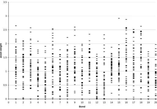
factor 10 outcomes of the portfolio were simulated, resulting in a total of 10000 portfolio loss scenarios. The CVaR, resulting from the target function of the optimization problem was determined at the 99.9 quantile level. In the two figures below, computed optimal asset weights are plotted based on 50 different simulation runs to obtain an empirical estimate of the loss distribution. In the first figure this is done without and in the second figure under usage of importance sampling. When applying importance sampling then a crude simulation run as described above without IS was used to get an approximate value of VaR. Asset weights are computed in absolute terms of their initial exposure.

0 0,5 1 1,5 2 2,5 3 3,5 0 1 2 3 4 5 6 7 8 9 10 11 12 13 14 15 16 17 18 19 20 Bond asset weig ht

Figure 1 : optimal asset weights, crude simulation

0 0,5 1 1,5 2 2,5 3 3,5 0 1 2 3 4 5 6 7 8 9 10 11 12 13 14 15 16 17 18 19 20 Bond asset weig ht

Optimal asset weights at a value of 0 are due to minimum restrictions at zero times of the initial bond exposure. It is obviously clear that usage of importance sampling results in a lower variability of asset weights. Narrow distributed optimal solutions for a single asset-weight follow from a reduced variance. Multiple solutions for a single asset-asset-weight result from repeatedly solving the stochastic optimization problem each based on a new importance sampled loss distribution.

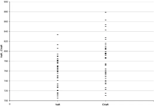
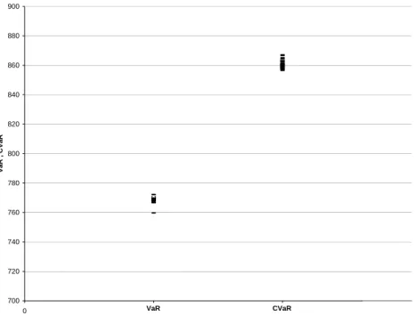
In the optimization procedure, CVaR is the value of the target function and VaR results as a byproduct of the optimization as part of the target function. Both values are plotted in the figures below again on the basis of 50 different simulation runs for the loss distribution with an optimization computed, each based on a unique simulation run. The first figure plots CVaR and VaR in a crude simulation setting. In the second figure importance sampling was additionally conducted. 700 720 740 760 780 800 820 840 860 880 900 0 1 2 3 VaR , CVaR VaR CVaR

700 720 740 760 780 800 820 840 860 880 900 0 1 2 3 VaR , CVaR VaR CVaR

Figure 4 : VaR , CVaR under (IS)

Here again variance reduction is obvious, exact figures are given in the table below.

The table shows the results for variance of estimates for CVaR and VaR as well as the asset weights with and without usage of importance sampling. Total asset weights variance is computed as sum of single asset weights’ variances of repeated optimization runs, each based on a new simulated loss distribution.

crude sampling _σˆ2 2192.25979 CVaR importance sampling _σˆ2 6.1842 crude sampling _σˆ2 1713.8852 VaR importance sampling _σˆ2 3.3933 crude sampling ∑_σˆ2 6.42681951

Asset-weights importance sampling ∑_σˆ2

0.01433357

Table 2

Obviously variances for CVaR and VaR as well as asset weights are lowered by means of importance sampling in our example by a factor of at least 350.

Above combination of importance sampling and stochastic optimization is closely related to bank practice when managing a credit portfolio. Searching for optimal portfolio hedging, optimal investment in credit default swaps or the amount of credit insurance can be

point for above outlined portfolio optimization. RiscMetrics’ CreditManager as one of the markets’ dominating credit portfolio models readily provides an implemented importance sampling technique. Besides the scenario output file consisting of explicit outcomes of each simulation run for the portfolio elements also the likelihood ratio corresponding to each loss scenario is part of the output, thus making an implementation of stochastic optimization with integrated importance sampling according to (5) fairly simple. In bank practice the scenario file as well as the likelihood ratios can be used as a basis to build up the above presented optimization model in a suitable programming language. The optimization problem itself has to be set up in some matrix generator as SAS or Matlab that might already be available. The resulting large scale LP problem can be solved using programs as SAS, Cplex or Mosek. The only restricting factors then become the capabilities of the bank’s risk model in terms of accuracy and credit-products implemented.

Conclusion

It is shown that optimal asset weights in a stochastic CVaR credit portfolio optimization model may be exposed to a high degree of variability, making a high number of simulations necessary to achieve satisfactory results. Often memory resources are limited and problem size may outreach those limits. Importance sampling is a helpful tool to attain an acceptable degree of asset weight volatility at a feasible size of the problem. The integration of importance sampling techniques according to Glasserman and Li (2005) into the linear stochastic optimization problem formulized by Uryasev and Rockafellar (2001) is proposed. In a sample case pretty good results were achieved. Mapping the findings to bank practice it was noted that standard software as for example RiscMetrics’ CreditManager is readily delivering the necessary input for building an optimization model augmented by means of importance sampling. The portfolio steering eligibility of the outlined optimization procedure then becomes dependent on the capabilities of the bank’s risk model by accuracy and credit-products implemented.

References

Acerbi, C., Tasche, D. (2002): On the coherence of Expected Shortfall. Journal of Banking & Finance, Vol. 26, No. 7, P. 1487-1503.

Andersson, F., Mausser, H., Rosen, D., Uryasev, S. (2001): Credit Risk Optimization with Conditional Value-at-Risk Criterion. Mathematical Programming, Series B, Vol. 89, No. 2, P. 273-291.

Artzner, P., Delbaen, F., Eber, J.-M., Heath, D., (1999): Coherent Measures of Risk. Mathematical Finance,Vol. 9, No. 3, P. 203-228.

Dunkel, Jörn, Weber, Stefan (2005) Efficient Monte Carlo Methods for Convex Risk Measures in Portfolio Credit Risk Models. Working Paper, Columbia University.

Glasserman, Paul, (2003): Monte Carlo Methods in Financial Engineering. Spinger, New York.

Glasserman, Paul, Li, Jingyi (2005): Importance Sampling for Portfolio Credit Risk. Management Science, Vol.51, No. 11, P. 1643 - 1656.

Glasserman Paul (2005): Measuring Marginal Risk Contributions in Credit Portfolios. Working Paper, Columbia Business School.

Gupton, Greg M., Finger, Christopher C., Bhatia, Mickey, (1997): CreditMetrics-Technical Document, Morgan Guaranty Trust Company.

Markowitz, H. M. (1952): Portfolio Selection, Journal of Finance, Vol. 7, Iss. 1, P. 77-91. Rockafellar, R.T, Uryasev, S. (2001): Optimization of Conditional Value-at-Risk. The Journal of Risk, Vol. 2, No. 3, P. 21-41.

Rockafellar, R.T, Uryasev, S. (2002): Conditional Value-at-Risk for general loss distributions. The Journal of Banking & Finance, Vol. 26, No. 7, P. 1443-1471.

Szegö, Giorgio (2002): Measures of Risk, Journal of Banking and Finance. Vol. 26, No. 7, P. 1253-1272.

Xiao, Jerri , Yi (2002): Importance Sampling for Credit Portfolio Simulation, RiskMetrics Journal, Winter 2002.