Research Article Sliding Mode Control of Discrete Chaotic System Based on Multimodal Function Series Coupling

(1)

Research Article

Sliding Mode Control of Discrete Chaotic System Based on

Multimodal Function Series Coupling

Fengjun Hu

Institute of Information Technology, Zhejiang Shuren University, Hangzhou, Zhejiang 310014, China Correspondence should be addressed to Fengjun Hu; [email protected]

Received 9 December 2016; Revised 2 March 2017; Accepted 20 March 2017; Published 12 April 2017

Academic Editor: Eric Campos-Canton

Copyright © 2017 Fengjun Hu. This is an open access article distributed under the Creative Commons Attribution License, which permits unrestricted use, distribution, and reproduction in any medium, provided the original work is properly cited.

A new sliding mode control model of discrete chaotic systems based on multimodal function series coupling is proposed to overcome the shortcomings of the standard PSO algorithm in multimodal function optimization. Firstly, a series coupled PSO algorithm (PP algorithm) based on multimodal function is constructed, which is optimized by multipeak solution on the basis of the standard PSO algorithm. Secondly, the improved PSO algorithm is applied to search all the extreme points in the feasible domain. Thirdly, the Powell method is used to perform the local optimization of the search results, and the newly generated extreme points are added to the extreme point database according to the same peak judgment operator. Finally, the long training time of PP algorithm can be overcome by the characteristics of fast convergence rate of the cloud mutation model. And also, both the population size and the redundancy can be reduced. Then, the clonal selection algorithm is used to keep the diversity of the population effectively. Simulation results of the sliding mode control of discrete chaotic systems show that the improved PSO algorithm obviously improves the response speed, overshoot, and so on.

1. Introduction

Chaotic system can be divided into integer order chaotic system and fractional chaotic system. Fractional chaotic system is a very complex nonlinear system [1]. Sliding mode control has become an important branch of modern control theory because of its good robustness and antijamming characteristics [2]. Fractional chaotic system sliding mode has advantages of fractional chaotic system and sliding mode control, which can further improve the control performance of the system on the basis of traditional sliding mode control and become an important research area of modern nonlinear control.

Before introducing the sliding mode control of fractional order chaotic system, we mainly studied the control and syn-chronization of the fractional chaotic systems. At present, the control and synchronization of the fractional chaotic system are divided into two categories. One is the classical system stability theory and control method based on traditional integer order system. On the basis of the theory and control method, the stability analysis of the fractional order is carried

out to design the integer order controller [3]. The other is to utilize the characteristics of the fractional order system to put forward the fractional order controller design method; then, the control of the fractional order system can be realized [4]. The control methods can be divided into the following areas: (1) Feedback control based on pole placement of the fractional order system: Matignon [5] discussed the relationship between internal stability and external stability of the fractional differential equations. The system is linearized near the equilibrium point. And the author also described the characteristic equation of the system and the eigenvector based on the frac-tional calculus theory and the tradifrac-tional algebraic polynomial, analyzed the relationship between the fractional system eigenvalues and the system matrix pole, and presented the sufficient conditions for the stability of the fractional order system.

(2) The control of Gronwall inequality based on the frac-tional order: the Gronwall inequality is extensively applied to the integer order differential equation, and

Volume 2017, Article ID 8423413, 11 pages https://doi.org/10.1155/2017/8423413

(2)

the solution of the system is expressed analytically. The Gronwall inequality is taken to analyze the system solution to obtain the design of the controller, which is a common control design method for integer order systems. Lazarevi´c and Spasi´c [6] applied the Gron-wall inequality to the fractional time-delay system, analyzed the solution of the fractional order system, and realized the finite-time stabilization control of the fractional order. N’Doye and others [7] generalized the Bellman-Gronwall inequality, analyzed a class of nonlinear affine fractional order systems, and achieved the asymptotic stability of the fractional systems. Ye et al. [8] extended the integer order Gron-wall inequality to the fractional systems, proposed the generalized Gronwall inequality, and successfully implemented the asymptotic stability control for the fractional time-delay systems.

(3) Fractional order PID control: in the classical control theory and applications, PID controller has been de-veloped very well and is widely applied to the actual system. In accordance with the PID control, the integral controller and differential controller of the PID controller can be partially extended to the frac-tional order; that is, the fracfrac-tional integral and the fractional differential are introduced into the control design. Vasundhara Devi et al. [9] first proposed the fractional order PID controller and proved that the integer order PID controller belongs to a subset of the fractional PID controller. By adjusting the fractional order, the control effect of the fractional integral and fractional differential controller can be changed. (4) Feedback control based on linear matrix inequality:

Sabatier and others [10] gave a sufficient and neces-sary condition for the stability of the fractional order time-invariant interval uncertain systems. Because of the state boundedness characteristic of chaotic systems, this condition has been applied to the control and synchronization of the fractional order chaotic systems. Chen and others [11] presented a sufficient and necessary condition for the fractional order systems with parametric perturbations and applied it to the fractional order chaotic systems to achieve robust synchronization of the fractional order chaotic systems. Dadras and Momeni [2] introduced the passive theory into the fractional order system and designed the fractional integral sliding surface by the linear matrix inequality to realize the passive sliding mode control of the time-varying uncertain fractional chaotic systems.

(5) Sliding mode control of the fractional order system: the application of the integer order sliding mode to the fractional systems has been proved to be effective. The integral sliding mode surface and approach law are designed, respectively. And the effectiveness of the sliding surface is proved. The Lyapunov function is designed to analyze the stability of the fractional order system, and then, the sliding mode control law is obtained [12]. On the other hand, by combining

the design idea of the integral sliding mode surface with the characteristics of the fractional system, we can design the fractional sliding mode surface, and the integer integral of the sliding surface is changed to the fractional integral [13]. Similarly, the approximation of the integer order can be extended to the fractional systems; that is, the differential equation of integer order approximation law description can be generalized into the fractional order equation, which can realize the fractional order sliding mode approximation law [14].

In this paper, a PSO multiobjective optimization algo-rithm is introduced. Since the algoalgo-rithm is easy to fall into the local optimization, a sliding mode control of discrete chaotic system based on multimodal function series coupling is pro-posed combining the characteristics of multimodal function optimization problems. Simulations show the effectiveness of this method.

2. Multimodal Function Optimization

Problem Modeling

In many engineering optimization, such as complex sys-tem parameters and structural optimization, neural network weights, and structural optimization, we not only need to find the global optimal solution in the feasible region but also need to search several global optimal solutions and other valued local optimal solutions. Thus, multichoices and multi-information can be provided for decision makers. The above can be classified as multimodal function optimization problem or multipeak function optimization (MFO).

The multimodal optimization problem, as shown in (1), consists of two parts: the objective function and the search range.

Minimize 𝑓 (𝑥) , 𝑥 = (𝑥₁, 𝑥₂, . . . , 𝑥_𝑛) ∈ 𝑆. (1) In (1), the search range𝑆that can meet all the variables is called the feasible region, and the solution in feasible region is called the feasible solution. In the feasible region, the solution with the smallest objective function is the optimal solution. The optimal solution can be divided into global optimal solution and local optimal solution. In the multimodal function optimization, not only all the global optimal solutions of the optimization problem need to be found, but also the local optimal solutions need to be found as many as possible.

For the MFO problem of the objective function minimum value solution, the fitness function is defined as

fit(𝑋) = 𝑓 (𝑋) . (2)

In (2),𝑓(𝑋)is the function value of𝑋, and fit(𝑋)is the fitness value.

For the MFO problem of the function maximum value solution, the limit construction method is used to solve the minimization problem. The fitness function is defined as

(3)

In (3),𝐶maxis the maximum estimate of𝑓(𝑋).

From (2) and (3), we can see that the smaller the fitness value, the better the fitness.

3. Solution Algorithm of Multimodal Function

Problem Based on Series Coupling

Based on PSO algorithm and Powell method, this paper presents PP algorithm based on series coupling. The PP algorithm has the maximum repetition search𝑀(𝑀 > 1) to avoid the situations in which not all the extreme values can be searched in an evolutionary iteration. In each iteration, firstly, the improved PSO algorithm is used to carry out the global search of all the extreme points in the feasible region. Secondly, Powell method is used to perform the local search towards the optimal solutions found by the improved PSO to improve the accuracy of the solution. Finally, the peak judgement operator adds the newly generated extreme points to the extreme point database and rerandomizes the initialization of the particles.

3.1. PSO Algorithm Improvement. In the case of the par-ticle swarm with the 𝑁 numbers of particles in the D -dimensional search space, denote the flying speed of particle

𝑖as𝑉_𝑖 = (𝑉_𝑖1, 𝑉_𝑖2, . . . , 𝑉_𝑖𝐷)𝑇. The current position is𝑋_𝑖 =

(𝑋_𝑖1, 𝑋_𝑖2, . . . , 𝑋_𝑖𝐷)𝑇_{, the searched optimal position of particle}

𝑖is𝑃_𝑖 = {𝑃_𝑖1, 𝑃_𝑖2, . . . , 𝑃_𝑖𝐷}, and the searched optimal position

of the swarm is𝑃_𝑔 = {𝑃_𝑔1, 𝑃_𝑔2, . . . , 𝑃_𝑔𝐷}. In order to reduce the possibility of the particles leaving the search space during the process of evolutionary iterations, the speed is limited as

𝑉min ≤ 𝑉𝑖𝑑≤ 𝑉max. The standard PSO is shown in

𝑉_𝑖𝑑(𝑡 + 1) = 𝜔 (𝑡) 𝑉_𝑖𝑑(𝑡) + 𝑐₁rand()(𝑃_𝑖𝑑(𝑡) − 𝑋_𝑖𝑑(𝑡))

+ 𝑐₂rand()(𝑃_𝑔𝑑(𝑡) − 𝑋_𝑔𝑑(𝑡)) . (4) In (4),𝑡is the current iteration number,𝑉_𝑖𝑑represents the

𝑑th dimensional component of the particle𝑖velocity vector

𝑉, and 1 ≤ 𝑑 ≤ 𝐷. 𝑐₁ represents the cognitive learning factor of the particle individual and𝑐₂ represents the social learning factor. rand() is the random number generated by the uniform distribution on[0, 1].

In the multimodal optimization, in order to make each local optimal value become the “only way” of some particles in PSO algorithm, this paper improves the standard PSO and obtains the improved PSO.

(1) Ideally, the self-cognition of each individual in the particle swarm represents each local optimization of the multipeak optimization. Thus, let𝑐₂ = 0; we can obtain not just the global optimal values, but all the local optimal values.

(2) Consider that the random function rand() in (4) mainly increases the randomness of the particle motion so as to make the local optimal point jump out. In order to let each particle of the particle swarm converge to each local optimal value as soon as possible, rand() in (4) should be removed.

(3) The linear decreasing strategy of inertia weight is simple and intuitive and has better searching ability, which makes the algorithm balance between the global search and the local search. Therefore,𝜔uses the above strategy, which is shown in

𝜔 (𝑡) = 𝜔start− (𝜔start− 𝜔end)

𝑡

𝑡max

. (5)

In (5),𝑡represents the current PSO iteration algebra,𝑡max

represents PSO maximum iteration number, and𝜔_start and

𝜔_endrepresent the maximum and the minimum value of𝜔. Based on the above improvements, (4) can be changed to

𝑉_𝑖𝑑(𝑡 + 1) = 𝜔 (𝑡) 𝑉𝑖𝑑(𝑡) + 𝑐1(𝑃𝑖𝑑(𝑡) − 𝑋𝑖𝑑(𝑡)) . (6)

The position change is performed according to (7). In order to avoid the particles leaving from the search space during the process of evolution iteration, the following condition should be satisfied:𝑋_min≤ 𝑋_𝑖𝑑≤ 𝑋_max.

𝑋_𝑖𝑑(𝑡 + 1) = 𝑋_𝑖𝑑(𝑡) + 𝑉_𝑖𝑑(𝑡 + 1) . (7)

3.2. Nonlinear Powell Direct Search Method. The nonlinear Powell direct search method is a nonlinear direct local search method for solving unconstrained optimization problems without using derivatives. It is considered to be a relatively effective method in direct search. Powell search method is known as the direction acceleration method as well. Using this method, the calculation of the derivative is not required and only the function value is used to carry out the one-dimensional search from one point towards two directions. Then, the minimal value can be obtained. Nonlinearity means that the search direction of the initial point is not fixed, the acceleration direction will change with the change of the initial point position, and the search is not along a straight line.

The steps of the Powell search method are as follows:

Begin

Step 1. The particle of the last search generation of PSO is taken as the initial point𝑥(0) ∈ 𝑆. Set the search precision of the Powell method as𝜀.𝐷numbers of initial linearly inde-pendent search directions𝑑(𝑖)are given, and𝑖 = 0, 1, . . . , 𝐷−1.

Set𝑘 = 0.

Step 2. According to (9) below, one-dimensional search is performed accurately from point𝑥(0)to each search direc-tion in turn𝑑(0), 𝑑(1), . . . , 𝑑(𝐷−1). Thus,𝑥(0), 𝑥(1), . . . , 𝑥(𝐷) is obtained. 𝑓 (𝑥(𝑖)+ 𝛼_𝑖𝑑(𝑖)) =min 𝛼∈𝑆𝑓 (𝑥 (𝑖)_{+ 𝛼𝑑}(𝑖)_{) ,} (8) 𝑥(𝑖+1)= 𝑥(𝑖)+ 𝛼_𝑖𝑑(𝑖). (9) In (8),𝛼and𝛼_𝑖represent the step sizes and𝛼_𝑖is obtained by the exact linear search; that is,𝛼_𝑖is the solution of the one-dimensional optimization problem above.𝛼_𝑖can be negative, which indicates that the exact linear search takes place over the entire real axis.

(4)

Step 3. Let𝑑(𝐷) = 𝑥(𝐷)− 𝑥(0). If‖𝑑(𝐷)‖ ≤ 𝜀, and the solution

𝑥(𝐷)_{is obtained, calculation ends. Otherwise, the exact linear}

search is performed from point𝑥(𝐷)to the direction of𝑑(𝐷) to get𝑥(𝐷+1).

Step 4. According to (10), the indicator𝑡𝑙determined by the maximal decrease is calculated.

𝑓 (𝑥(𝑡𝑙)) − 𝑓 (𝑥(𝑡𝑙+1))

= max

0≤𝑖≤𝐷−1{𝑓 (𝑥

(𝑖)_{) − 𝑓 (𝑥}(𝑖+1)_{)} .} (10)

Step 5. When (11) holds, it shows that𝑑(0), 𝑑(1), . . . , 𝑑(𝐷−1)are still linearly independent, and the search directions of the next round are still𝑑(0), 𝑑(1), . . . , 𝑑(𝐷−1). Then,𝑥(0) = 𝑥(𝐷+1). Return to Step 2.

𝑓 (𝑥(0)) − 2𝑓 (𝑥(𝐷)) + 𝑓 (2𝑥(𝐷)− 𝑥(0))

≥ 2 (𝑓 (𝑥(𝑡𝑙)) − 𝑓 (𝑥(𝑡𝑙+1))) . (11)

Step 6. When (11) does not hold, it shows that 𝑑(0),

𝑑(1)_{, . . . , 𝑑}(𝐷−1) _{are linearly dependent. Thus, set} _𝑑(𝑡𝑙+1) ₌

𝑑(𝑡𝑙+𝑖+1)to ensure linearly independence of the new generated search direction,𝑥(0)= 𝑥(𝐷+1),𝑘 = 𝑘 + 1. Return to Step 2.

End

3.3. The Same Peak Judgement of the Extreme Points. The extreme points found by the PP algorithm are compared with all the extreme points in the extreme point database EP in turn and make the same peak judgement. If it is judged as the same peak and greater than the fitness value of the existing extreme point, the extreme point is discarded. If it is judged as the same peak but less than the fitness value of the extreme point, the extreme point is replaced. And if it is judged to be different peak, it is added to set EP.

The same peak judgement operator uses the peak explo-ration method to perform the same peak judgement towards the global extreme points. In this paper, the peak exploration method is applied in the same peak judgement of all the global and local extreme points. The method is as follows.

Set𝐴as an extreme point in EP and𝐵as the extreme point found by the PP algorithm.(ℎ−1)points are inserted between

𝐴and𝐵, and𝐴𝐵is divided intoℎequal parts. The same peak operators ofℎparts are calculated, which is shown as

𝑇𝑓 (𝑖) =fit(𝑋_𝑖+1) −fit(𝑋_𝑖) . (12)

In (12),𝑋_𝑖+1 and𝑋_𝑖 are two adjacent points between𝐴

and𝐵, 1 ≤ 𝑖 ≤ ℎ. When𝑖 = 1, 𝑋₁ is point𝐴, and when

𝑖 = ℎ,𝑋_ℎ+1 is point𝐵. If value of𝑇𝑓changes from positive

to negative, it means that there is a mountain between points

𝐴and𝐵. Then,𝐴and𝐵are different peak extreme points. Otherwise, they are the same peak extreme points.

3.4. Performance Analysis of PP Algorithm in Multimodal Function Optimization Problem. Let the numbers of particles

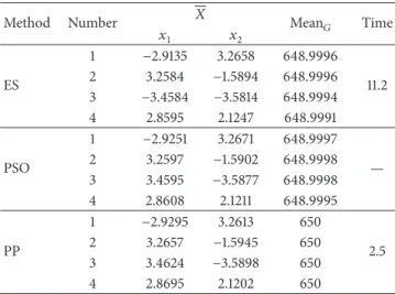
Table 1: Comparisons of PP algorithm with other evolutionary algorithms.

Method Number 𝑋 Mean_𝐺 Time

𝑥1 𝑥2 ES 1 −2.9135 3.2658 648.9996 11.2 2 3.2584 −1.5894 648.9996 3 −3.4584 −3.5814 648.9994 4 2.8595 2.1247 648.9991 PSO 1 −2.9251 3.2671 648.9997 — 2 3.2597 −1.5902 648.9998 3 3.4595 −3.5877 648.9998 4 2.8608 2.1211 648.9995 PP 1 −2.9295 3.2613 650 2.5 2 3.2657 −1.5945 650 3 3.4624 −3.5898 650 4 2.8695 2.1202 650

𝑁be 20∼105. Set the acceleration factor𝑐₁ = 1.49445. Set the inertia weight: 𝜔_start = 0.9, 𝜔_end = 0.4, and 𝑡_max =

30, respectively. The maximal repeated search number is

𝑀 = 2∼10, and 𝜀 = 2 × 10−8. Select 𝑓₁ as the test function; the comparison of the results of the PP algorithm, multipopulation coevolution strategy ES, and the standard PSO algorithm is shown in Table 1.

𝑓1(𝑥) = 660 − (𝑥21+ 𝑥2− 11)2− (𝑥1+ 𝑥22− 7)

2

. (13)

In Table 1,𝑋 represents the mean value of the optimal solution location at the time of the test. Mean_𝐺is the average of the global solutions of the 50 tests.

From Table 1, we can see that, compared with ES and the standard PSO, the PP algorithm can search all four global extreme points of the function𝑓₁in 50 tests, and also there are no redundant or missing extreme points. The solution quality is significantly improved. Therefore, the PP algorithm has obvious advantages in search precision.

For function𝑓₁, the standard PSO has no mean comput-ing time, and we use “—” to express time. Time of the ES is 11.2 seconds, and time of the PP algorithm is 2.5 seconds. Thus, the PP algorithm has obvious advantages in the speed of convergence.

Then, the global convergence of PP algorithm is analyzed.

Suppose. (1) Definition domainΩof the multimodal function optimization problem is a bounded closed region of𝑅𝑛. (2) The objective function𝑓(𝑋)is a continuous function on the regionΩ.

Theorem 1. Set{𝑋(𝑘)}(𝑘is the cumulative iteration algebra) as the population sequence generated by the PP algorithm, where𝑥∗(𝑘) ∈ 𝑋(𝑘)is the optimal point in the𝑘th generation of the population; that is,𝑥∗(𝑘) = arg min_𝑥∈Ω𝑓(𝑥(𝑘)). If the objective function and the feasible region of problem𝑃satisfy hypothesis 1,𝑝{lim_𝑘→∞𝑓(𝑥∗(𝑘)) = 𝑓∗} = 1holds, where

(𝑓∗ ₌ _min_{{𝑓(𝑥) : 𝑥 ∈ Ω})}_{; that is, the population sequence}

(5)

Demonstration. Define the cumulative iteration algebra𝑘as

𝑘 = 𝑡_max(𝑚 − 1) + 𝑡, where𝑚is the repeated search algebra

(1 ≤ 𝑚 ≤ 𝑀),𝑡_maxis the maximum iteration algebra, and𝑡is

the iterative algebra.

The change of the displacement of the two generations before and after the PP algorithm isΔ𝑋_𝑖𝑑(𝑡) = 𝜔(𝑡)𝑉_𝑖𝑑(𝑡) +

𝑐1(𝑃𝑖𝑑(𝑡) − 𝑋𝑖𝑑(𝑡)). Thus, when the population particles

converge, the social cognitive part (𝑃_𝑖𝑑(𝑡) − 𝑋_𝑖𝑑(𝑡)) tends to 0 and less than 1, the particle velocity will drop rapidly to 0, and the particle swarm will stop moving. Therefore, the population particles may converge on the local solution and not on the global solution. For this reason, when the population particles fall into the evolutionary stagnation state, the particles are subjected to the mutation operation through the basic normal cloud generator. And the basic normal cloud generator based on the cloud model is subject to normal distribution.

Due to the mutation operation of the basic normal cloud generator with normal distribution, the displacement of particle𝑋_𝑖is subject to normal distribution; that is,Δ𝑋_𝑖(𝑡) ∼

𝑁(0, 𝜎_𝑡2), where𝑁(0, 𝜎_𝑡2)represents the normal distribution

with average value 0 and variance𝜎_𝑡2.

Therefore, we can conclude that Theorem 1 holds.

4. Optimization of PP Algorithm Based on

Cloud Mutation Clonal Selection

In order to solve the problems of the multimodal function optimization, based on the above improved methods, this paper utilizes the characteristics of fast convergent speed of the cloud mutation model to compensate the shortcomings of fast training time of the PP algorithm. Meanwhile, it can reduce the population size and redundancy. And the clonal selection algorithm can effectively maintain the diversity of population. Hence, a particle swarm optimization algo-rithm based on cloud mutation clonal selection is proposed (WCPP).

4.1. Optimization of Particle Space Distribution Based on Cloud Mutation. The cloud model has the characteristics of randomness and stability tendency. The randomness can keep the individual diversity so as to search for more local extreme points, and the stable tendency can protect the better individual to perform adaptive localization of the global optimal values. Thus, in order to improve the accuracy of the PP algorithm and expand the search range to find other extreme points, a cloud mutation operator based on cloud model is introduced on the basis of the PP algorithm to update the particles.

Thresholds𝜀and𝑡_𝑁are given. When a particle satisfies (14), that is, the particle degenerates and degradation ampli-tude is smaller than𝜀, it is considered that the particle has a generation in the evolutionary stagnation state.

0 <fit(𝑋_𝑖(𝑡)) −fit(𝑋_𝑖(𝑡 − 1)) < 𝜀, (14)

𝜀 =abs(fit(𝑋𝑖(𝑡))

𝑎 ) . (15)

In (15), fit(𝑋_𝑖(𝑡))represents the fitness value of𝑋_𝑖in the

𝑡th generation.𝑎is a constant. When fit(𝑋_𝑖(𝑡)) −fit(𝑋_𝑖(𝑡 −

1)) < 0, it indicates the evolution of particle𝑋_𝑖. And when

fit(𝑋_𝑖(𝑡)) −fit(𝑋_𝑖(𝑡 − 1)) > 0, it indicates the degradation of

particle𝑋_𝑖.

The cloud mutation condition can be defined as the degradation of a particle of 𝑡_𝑁 successive generations and the degradation amplitude is less than 𝜀. When a particle satisfies the condition of cloud mutation, mutation operation is performed to the particle by a basic normal cloud generator.

𝑡_𝑁 is set as 5 here. Since𝑡_𝑁 is set too small, the mutation occurs too frequently and it is easy to miss the extreme point. On the other hand, the convergent speed of the algorithm can slow down.

One-dimensional normal cloud operator can be extended to𝐷dimensions. And the cloud mutation operator for each dimension of𝑋_𝑖is as follows:

Begin

For𝑑 = 1 : 𝐷

𝐸𝑥 = 𝑋_𝑖𝑑;

𝐸𝑛 =variable search range/𝑐𝑐1;

𝑐𝑐1 = 20sqrt(𝑡);

𝐻𝑒 = 𝐸𝑛/𝑐𝑐2;

𝑐𝑐2 = 10;

A normal random number𝑥_𝑖is generated by the basic normal cloud generator, at the same time a random number Temp is also generated. When𝜇_𝑖 > Temp,𝑋_𝑖𝑑 is updated by𝑥_𝑖.

End For End

𝐸𝑛represents the horizontal width of the cloud, and the greater the horizontal width, the greater the scope of the particle search. When 𝑐𝑐1 is set as 20sqrt(𝑡), the search range of the initial evolution is very large, which is helpful to find more extreme points. With the dynamic narrowing of the search range of𝑡, it is favorable to the fine search of particles.

“Dimensional catastrophe problem” exists in dimension function. As the dimension increases, it is difficult to find the optimal solution in each dimension through the general evolutionary algorithms. The abnormal values on individual dimension lead to poor quality of the final solution or an inability to find the optimal solution to the optimization problem. Thus, in order to prevent the particles from falling into the local extreme points and failing to find the global optimal solution in high-dimensional multimodal function, the search particles are reinitialized with a certain probability

𝑝_𝑠 to find better solutions. When in the search state, the particles are rerandomly distributed in the search space as shown in

𝑉_𝑘(𝑡 + 1) =(𝑉min+ 𝑉max)

2

(6)

𝑋_𝑘(𝑡 + 1) = (𝑋min+ 𝑋max)

2

+ (𝑋_max− 𝑋_min) (rand()− 0.5) 𝕜. (16) After the initialization, particles are updated according to (16).

4.2. Population Diversity Optimization Based on Clonal Selec-tion Algorithm. In order to ensure the diversity of the popula-tion, optimization is performed based on the clonal selection algorithm. The steps are divided into clonal amplification, adaptive wavelet mutation, and immune selection.

(1) Clonal Amplification. In the PSO immune system, the problem to be solved is the antigen. Each particle in the particle swarm has the potential to represent each local optimization value in the multipeak optimization. Therefore,

𝑁particles searched in the last iteration of the PP algorithm are all used as antibodies. The affinity function of antibodies and antigens uses the fitness function of the PP algorithm; that is,

affinity(𝑎_𝑖) =fit(𝑎_𝑖) . (17) In (17), fit(𝑎_𝑖) is the fitness value of particle 𝑎_𝑖 and affinity(𝑎_𝑖)is the affinity value of the antibody𝑎_𝑖(the particle

𝑋_𝑖). From (17), we can see that the smaller the affinity value of the antibody, the better the affinity.

The antibodies in the antibody population were sorted in ascending order according to the affinity value before the clonal amplification. The clonal amplification operator for the sorted𝑖th antibody𝑎_𝑖is calculated according to

𝛽_𝑖=round(𝑎_𝑐 1

√𝑖+ 𝑏) . (18)

In (18),𝑎_𝑐is a constant greater than 1, round()is a round function, and𝑏can ensure that each antibody has a constant larger than 1 with a certain number of clones. From (18), we can see that the higher the affinity, the greater the clonal multiple. In the clonal selection algorithm, when the current iteration number is ct, the𝑖th cloned amplified antibody𝑎_𝑖is changed to𝑎_𝑖(ct) = {𝑎_𝑖1(ct), 𝑎_𝑖2(ct), . . . , 𝑎_𝑖𝛽𝑖(ct)}after𝛽_𝑖times of clone.

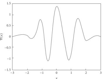
(2) Adaptive Wavelet Mutation. Morlet wavelet has better probability distribution of upper and lower wings. Thus, Morlet wavelet is applied to immune mutation operation to make CSA have a wider range of searching, higher precision, and good regulating performance. Morlet wavelet mother function is shown in

Ψ_𝑎,𝑏(𝑥) = 1

√𝑎𝑒−((𝑥−𝑏)/𝑎)/2cos(5 𝑥 − 𝑏

𝑎 ) . (19)

When𝑎 = 1and𝑏 = 0, Morlet wavelet function is shown

in Figure 1. In Figure 1, the horizontal axis is the independent variable, and the vertical axis is the wavelet mother function.

−1.5 −1 −0.5 0 0.5 1 1.5 −3 −2 −1 0 1 2 3 x Ψ( x)

Figure 1: Morlet wavelet function.

With the progress of ct, the affinity of the antibody increases constantly. When the adaptive dynamic of the antibody mutation probability 𝑝_𝑚 reduces, the convergent speed of the algorithm can be improved.𝑝_𝑚is shown as

𝑝_𝑚(ct) = 𝑝_𝑚(ct− 1) (1 − 0.01 ct

ct_max) . (20) In (20), ct_max is the maximum iteration number. When ct= 1, the initial value is set as 0.7.𝑋_𝑖𝑑mutation uses adaptive wavelet mutation operator based on the time-varying scale.

𝑋_𝑖𝑑mutation formula is shown as follows:

𝑋󸀠_𝑖𝑑= {𝑋_𝑖𝑑+𝑋max− 𝑋𝑖𝑑

𝑚 𝜂 (ct) 𝜎 (ct) , 𝜎 (ct) ≥ 0𝑋𝑖𝑑

+𝑋𝑖𝑑− 𝑋min

𝑚 𝜂 (ct) 𝜎 (ct) ,else,

(21)

where𝑚is an increase constant.

𝜂 (ct) = 1 − 𝑟(1−ct/ctmax)𝑏. (22)

In (22), 𝜂(ct) is the time-based mutation scale, 𝑟 is the random number between [0, 1], and 𝑏 is the system parameter, which determines the dependency degree of the random number disturbance on ct.

𝜎 (ct) = 1

√𝑎 (ct)𝑒

−(𝜑/𝑎(ct))2/2_cos₍₅ 𝜑

𝑎 (ct)) . (23)

In (23),𝜎(ct)is the wavelet mutation function, and𝜑is a random number between[−3𝑎(ct), 3𝑎(ct)]. Function𝑎(ct)is shown as

𝑎 (ct) = 𝑒−ln(𝑔)(1−ct/ctmax)𝑐+ln(𝑔). ₍₂₄₎

In (24),𝑐is the shape parameter of𝑎(ct)and is set to 1.𝑔 is the upper limit of𝑎(ct)and is set to 10000. Thus, the value of𝑎(ct)increases with the increase of ct between 1 and 10000, while the range of𝜎(ct)shrinks with the increase of ct.

(7)

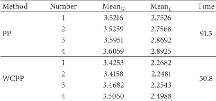
Table 2: Comparing the results of PP algorithm with WCPP algorithm.

Method Number Mean_𝐺 Mean_𝐿 Time

PP 1 3.5216 2.7526 91.5 2 3.5259 2.7568 3 3.5951 2.8692 4 3.6059 2.8925 WCPP 1 3.4253 2.2682 50.8 2 3.4158 2.2481 3 3.4682 2.2543 4 3.5060 2.4988

From (21), we can see that, at the early stage of the evolution, for smaller𝑟,𝜂(ct) ≈ 1. When the value of𝜎(ct)is large, the mutation space is also large, so that the probability of searching other extreme points can be increased. And in the middle and late stages of the evolution, adaptive of𝜂(ct) is smaller. When ct is approaching ct_max, 𝜂(ct) ≈ 0, and the value of𝜎(ct)is relatively small. Thus, by improving the local fine-tuning ability, the precision of the algorithm can be improved effectively.

(3) Immune Selection. Let 𝑆_𝑖(ct) = 𝑇_𝑠𝑐(𝑎_𝑖(ct)) = min{affinity(𝑎󸀠_𝑖(ct))}, and𝑆_𝑖(ct) ∪ 𝑎_𝑖(ct) → 𝑎_𝑖(ct+ 1).𝑎_𝑖󸀠(ct) represents an antibody obtained by clonal amplification and mutation of the ctth iteration. Compression of population antibody is achieved by local selection, and the optimal solution of population is not deteriorated.

4.3. Performance Analysis of WCPP Algorithm in Multimodal Function Optimization. Select𝑓₂as test function, the result comparison of the PP algorithm and the WCPP algorithm is shown in Table 2.

𝑓₂(𝑥) = 𝑥sin(10𝜋𝑥) + 2. (25)

In Table 2,𝑋 represents the mean value of the optimal solution location at the time of the test. Mean_𝐺represents the average of the global solutions of the 50 tests.

The mean value Mean_𝐿 of the local solution of the PP algorithm is larger than that Mean_𝐿of the WCPP algorithm, which shows that the local solution of the PP algorithm has higher accuracy than the WCPP algorithm in the case that 16 local extreme points can be searched for objective function

𝑓₂.

5. Application of WCPP Algorithm to Sliding

Mode Control of Discrete Chaotic Systems

5.1. Fractional Order Chaotic System Sliding Mode Control Model. Suppose a control system as ̇𝑥 = 𝑓(𝑥, 𝑢, 𝑡),𝑥 ∈ 𝑅𝑛,

𝑢 ∈ 𝑅𝑛_,_{𝑡 ∈ 𝑅}_{. Switching function needs to be determined,}

𝑠(𝑥), 𝑠 ∈ 𝑅𝑚. Then, the control function can be solved as

follows:

𝑢 = {𝑢+_{(𝑥) , 𝑠 (𝑥) > 0𝑢}−_{(𝑥) , 𝑠 (𝑥) < 0.} ₍₂₆₎

In (26),𝑢+(𝑥) ̸= 𝑢−(𝑥). Then,

(1) the sliding mode exists: that is, (26) holds;

(2) the accessibility condition can be satisfied, and the movement points outside the switching surface will reach the switching surface with a limited time; (3) the stability of the sliding mode movement is ensured; (4) the dynamic quality requirement of the control

sys-tem is satisfied.

If the first three basic problems can be satisfied, we can call the control as sliding mode control.

Henon fractional chaotic system is taken as an example; the sliding mode control model of fractional chaotic system is constructed. The Henon chaotic system with control is shown as

𝑥₁(𝑘 + 1) = 1 − 𝑎 (𝑥1(𝑘))2+ 𝑏𝑥2(𝑘) + 𝑢 (𝑘) ,

𝑥₂(𝑘 + 1) = 𝑥1(𝑘) ,

(27) where𝑥 ∈ 𝑅𝑛,𝑢 ∈ 𝑅.

Define the switching function as𝑠(𝑘) = 𝐶_𝑒[𝑒(𝑘), 𝑑𝑒(𝑘)], where𝐶_𝑒 = [𝑐_𝑘, 𝑐₀]. Then,𝑠(𝑘 + 1) = 𝐶_𝑒[𝑒(𝑘 + 1), 𝑑𝑒(𝑘 + 1)],

𝑑𝑒(𝑘 + 1) = (𝑒(𝑘 + 1) − 𝑒(𝑘))/ts, where ts is the sampling time.

And we can obtain (28) as follows:

𝑠 (𝑘) = 𝑐𝑘𝑒 (𝑘) + 𝑐0𝑑𝑒 (𝑘) ,

𝑠 (𝑘 + 1) = (𝑐𝑘+𝑐_ts0) 𝑒 (𝑘 + 1) − (𝑐_ts0) 𝑒 (𝑘) .

(28)

When the fractional order chaotic system enters the ideal sliding mode,𝑠(𝑘)can satisfy the following:

𝑠 (𝑘 + 1) = 𝑠 (𝑘) . (29) That is, (𝑐_𝑘+𝑐0 ts) 𝑒 (𝑘 + 1) − ( 𝑐₀ ts) 𝑒 (𝑘) = 𝑐𝑘𝑒 (𝑘) + 𝑐0𝑑𝑒 (𝑘) , (30) where𝑒(𝑘 + 1) = 𝑟(𝑘 + 1) − 𝑥₁(𝑘 + 1). Define𝑓(𝑘) = 1 − 𝑎𝑥2

1(𝑘) + 𝑏𝑥2(𝑘); then, we can have𝑢eq(𝑘) = 𝑥1(𝑘 + 1) − 𝑓(𝑘).

From the above, we can obtain the sliding mode control equivalent control part of the fractional order chaotic system

𝑢eq(𝑘), which is shown in

𝑢eq(𝑘)

=(𝑐𝑘+ 𝑐0/ts) 𝑟 (𝑘 + 1) − (𝑐𝑘+ 𝑐0/ts) 𝑒 (𝑘) − 𝑐0𝑑𝑒 (𝑘)

𝑐_𝑘+ 𝑐₀/ts .

(31)

5.2. Sliding Mode Control Flow of the Discrete Chaotic System Based on WCPP Algorithm

(1) Evaluation Function Selection.The selection of the evalua-tion funcevalua-tion not only needs to consider the stability, fastness, and accuracy of the system but also needs to consider the control energy problem, the form of which is shown as

𝐽 (𝑝) = ∫∞

(8)

In (32),𝑒(𝑡)is the system error,𝑢(𝑡)is the control variable,

𝑡_𝑢 is the initial step time, and𝑤₁, 𝑤₂, 𝑤₃ are the weights. The smaller the value of the evaluation function 𝐽(𝑝) is, the closer the corresponding function 𝑝 is to the global optimal solution. The evaluation function value decreases as the algorithm runs.

(2) Sliding Mode Control Flow of the Discrete Chaotic System Based on WCPP Algorithm. By using the WCPP algorithm, the parameters of the sliding mode controller are globally optimized to construct the sliding mode control method. The flow is as follows:

Begin

Step 1. Initialize the sliding mode controller, other parame-ters, and a group of particles with size𝑁. The initialization parameters include maximum repetition search number𝑀 of hybrid algorithm and the WCPP maximum number of iterations ct_max.

Step 2. The evaluation function value of each particle is obtained by control of the discrete chaotic system according to the position of each particle and the optimal position of individual particle𝑃_𝑖and the optimal position of all particles

𝑃_𝑔are recorded.

Step 3. If the repeated search algebra𝑚is larger than𝑀, the iteration is stopped, and the algorithm is finished. The output of the sliding mode controller controls the discrete chaotic system. Otherwise, turn to Step 4.

Step 4. Ifthe WCPP algorithm iteration number𝑡 ≤ 𝑡max,

Ifthe condition of the cloud mutation is satisfied,

the cloud mutation is performed on the particles.

Else

Speed and positions are updated on the particles.

End If

Update particles𝑃_𝑖and𝑃_𝑔, and

𝑡 + 1.

End If

Step 5. The particles in the last search generation of the WCPP algorithm are cloned and amplified.

Adaptive wavelet mutation operator performance is car-ried out.

Immune selection performance is carried out. And, ct+ 1.

End If

update particles𝑃_𝑖and𝑃_𝑔,

Step 6. 𝑚 + 1, the positions and the speed are reinitialized.

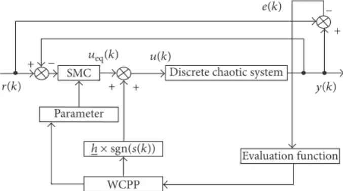
SMC Discrete chaotic system

Evaluation function WCPP Parameter e(k) y(k) u(k) ueq(k) r(k) − × sgn(s(k)) + + + + − ℎ

Figure 2: Sliding mode control of discrete chaotic system based on WCPP algorithm.

Step 7. The searched optimal fitness particles are assigned to the initialized particles and turn to Step 2.

End

In order to improve the fastness of the sliding mode control method for the discrete chaotic systems based on the WCPP algorithm, the values of the algorithm parameters𝑁 and𝑀are small.

Figure 2 is the discrete chaotic system sliding mode control structure based on the WCPP algorithm.

5.3. Algorithm Simulations. A discrete chaotic system is taken as the simulation object; the model of the controlled object is shown as

𝑦 (𝑘 + 1) = 𝑦 (𝑘)

1 + 𝑦 (𝑘)2_{+ 𝑑 (𝑘)}+ 𝑢 (𝑘)3. (33)

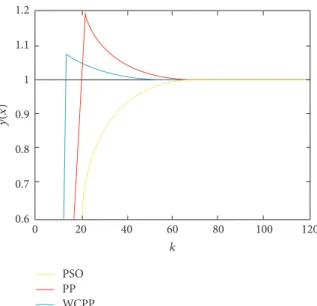
For the above discrete chaotic system, simulations of step input signal𝑟(𝑘) = 1are implemented based on the WCPP and other two algorithms, which is shown in Figure 3. In this simulation, the disturbance signal is set as𝑑(𝑘) = 0. And at this time the WCPP optimized parameters are{20, 1}.

From Figure 3, we can see that the WCPP algorithm has very strong search ability. It can search the global optimal value of the sliding mode controller parameters without overshoot, and the error, the response speed, and adjustment time all achieved the optimal performance. Therefore, the control effect of the WCPP algorithm is superior to the control effect of the PSO and the PP algorithm.

For the above discrete chaotic system, the simulations of the square wave input signal𝑟(𝑘) = 0.5sign(sin(8𝜋𝑘 ⋅ts)) are implemented by the WCPP algorithm and other two algorithms, respectively, which is shown in Figure 4.

Another discrete chaotic system is also taken as the simulation object; the model of the controlled object is shown as

𝑦 (𝑘) = −0.1𝑦 (𝑘 − 1) + 𝑢 (𝑘 − 1)_{1 + 𝑦}₂_{(𝑘 − 1)} . (34)

For the above discrete chaotic system, simulations of step input signal𝑟(𝑘) = 1are implemented based on the WCPP

(9)

1.2 1.1 1 0.9 0.8 0.7 0.6 0 20 40 60 80 100 120 k PSO PP WCPP y( x)

Figure 3: Simulation results of discrete chaotic systems.

0.5 0 −0.5 0 500 k PSO y( x) (a) PP 0.5 0 y( x) −0.5 0 500 k (b) WCPP 0.5 0 0 500 k −0.5 WCPP y( x) (c)

(10)

PSO PP WCPP y( x) 20 40 60 80 100 120 0 k 0.6 0.7 0.8 0.9 1 1.1 1.2

Figure 5: Simulation results of discrete chaotic systems.

0.5 0 PSO −0.5 0 500 k y( x) (a) 0.5 0 PP −0.5 0 500 k y( x) (b) 0.5 0 WCPP −0.5 0 500 k y( x) (c)

(11)

and other two algorithms, which is shown in Figure 5. The WCPP optimized parameters are{1.000, 0.001}.

From Figure 5, we can find that the WCPP algorithm is basically no overshoot and is able to achieve the desired value in the second iteration. The performances of the WCPP algorithm in error, response speed, and adjustment time are significantly better than those of PSO and PP algorithms. Therefore, WCPP algorithm has strong searching ability and good control quality.

For the above discrete chaotic system, the simulations of the square wave input signal𝑟(𝑘) = 0.5sign(sin(8𝜋𝑘 ⋅ts)) are implemented by the WCPP algorithm and other two algorithms, respectively, which is shown in Figure 6.

It can be seen from Figures 4 and 6 that the response speed, overshoot, and other performances of the WCPP algorithm have been improved significantly.

6. Conclusions

Chaos and chaos systems are widely used in physics, engi-neering, biology, finance, and so forth. The modeling of complex systems based on the theory of calculus can more accurately reflect the dynamic characteristics of the systems. Discrete chaotic systems can be widely used in the field of chaotic secure communications. Thus, it is of great theoretical and applicable value in the applications of control and synchronization of the chaotic dynamic systems. In order to overcome the shortcoming of the standard PSO algorithm in multimodal function optimization problems, a sliding mode control model of discrete chaotic systems based on the coupled multimode functions is proposed. The simulation results show that the improved algorithm proposed in this paper has significantly improved the response speed and overshoot performance compared with the standard PSO algorithm.

Conflicts of Interest

The author declares that there are no conflicts of interest regarding the publication of this paper.

Acknowledgments

This work was supported by the National Natural Science Foundation of China (Grant no. 51675490).

References

[1] Y.-H. Chang, C.-I. Wu, H.-W. Lin, H.-C. Chen, and C.-W. Chang, “Fractional order integral sliding-mode flux observer for direct field-oriented induction machines,” International Journal of Innovative Computing, Information and Control, vol. 8, no. 7, pp. 4851–4868, 2012.

[2] S. Dadras and H. R. Momeni, “Fractional terminal sliding mode control design for a class of dynamical systems with uncer-tainty,”Communications in Nonlinear Science and Numerical Simulation, vol. 17, no. 1, pp. 367–377, 2012.

[3] A. H. J. De Ruiter, “Adaptive spacecraft attitude control with actuator saturation,”Journal of Guidance, Control, and Dynam-ics, vol. 33, no. 5, pp. 1692–1696, 2010.

[4] H. Liu, L. Guo, and Y. Zhang, “Composite attitude control for flexible spacecraft with simultaneous disturbance attenuation and rejection performance,”Proceedings of the Institution of Mechanical Engineers. Part I: Journal of Systems and Control Engineering, vol. 226, no. 2, pp. 154–161, 2012.

[5] D. Matignon, “Stability properties for generalized fractional differential systems,”ESAIM: Proceedings and Surveys, vol. 5, pp. 145–158, 2008.

[6] M. P. Lazarevi´c and A. M. Spasi´c, “Finite-time stability analysis of fractional order time-delay systems: gronwall’s approach,” Mathematical and Computer Modelling, vol. 49, no. 3-4, pp. 475– 481, 2009.

[7] I. N’Doye, M. Zasadzinski, M. Darouach, and N.-E. Radhy, “Observer-based control for fractional-order continuous-time systems,” inProceedings of the 48th IEEE Conference on Decision and Control held jointly with 28th Chinese Control Conference (CDC/CCC ’09), pp. 1932–1937, December 2009.

[8] H. Ye, J. Gao, and Y. Ding, “A generalized Gronwall inequality and its application to a fractional differential equation,”Journal of Mathematical Analysis and Applications, vol. 328, no. 2, pp. 1075–1081, 2007.

[9] J. Vasundhara Devi, F. A. Mc Rae, and Z. Drici, “Variational Lya-punov method for fractional differential equations,”Computers & Mathematics with Applications, vol. 64, no. 10, pp. 2982–2989, 2012.

[10] J. Sabatier, M. Moze, and C. Farges, “LMI stability conditions for fractional order systems,”Computers & Mathematics with Applications, vol. 59, no. 5, pp. 1594–1609, 2010.

[11] Y. Chen, H.-S. Ahn, and I. Podlubny, “Robust stability check of fractional order linear time invariant systems with interval uncertainties,”Signal Processing, vol. 86, no. 10, pp. 2611–2618, 2006.

[12] T. P. Sales, D. A. Rade, and L. C. G. De Souza, “Passive vibra-tion control of flexible spacecraft using shunted piezoelectric transducers,”Aerospace Science and Technology, vol. 29, no. 1, pp. 403–412, 2013.

[13] J. Erdong and S. Zhaowei, “Passivity-based control for a flexible spacecraft in the presence of disturbances,”International Jour-nal of Non-Linear Mechanics, vol. 45, no. 4, pp. 348–356, 2010. [14] K. Lu, Y. Xia, Z. Zhu, and M. V. Basin, “Sliding mode attitude

tracking of rigid spacecraft with disturbances,”Journal of the Franklin Institute. Engineering and Applied Mathematics, vol. 349, no. 2, pp. 413–440, 2012.

(12)

Submit your manuscripts at

https://www.hindawi.com

Hindawi Publishing Corporation

http://www.hindawi.com Volume 2014

Mathematics

Journal of

Mathematical Problems in Engineering

Hindawi Publishing Corporation http://www.hindawi.com

Differential Equations

International Journal of Volume 2014

http://www.hindawi.com Volume 2014 Hindawi Publishing Corporationhttp://www.hindawi.com Volume 2014

Mathematical PhysicsAdvances in

Complex Analysis

Journal of

Optimization

Journal of

Combinatorics

International Journal of

Journal of

Function Spaces

Abstract and Applied Analysis

http://www.hindawi.com Volume 2014 International Journal of Mathematics and Mathematical Sciences

Hindawi Publishing Corporation http://www.hindawi.com Volume 201

The Scientific

World Journal

Discrete Dynamics in Nature and Society

#HRBQDSDĮ,@SGDL@SHBR

Journal of

http://www.hindawi.com Volume 2014 Hindawi Publishing Corporationhttp://www.hindawi.com Volume 2014

Stochastic Analysis

International Journal of