Optimal Bayesian Transfer Learning for Classification and Regression

(1)

OPTIMAL BAYESIAN TRANSFER LEARNING FOR CLASSIFICATION AND REGRESSION

A Dissertation by

ALIREZA KARBALAYGHAREH

Submitted to the Office of Graduate and Professional Studies of Texas A&M University

in partial fulfillment of the requirements for the degree of DOCTOR OF PHILOSOPHY

Chair of Committee, Edward R. Dougherty Co-Chair of Committee, Ulisses Braga-Neto Committee Members, Xiaoning Qian

Krishna Narayanan Anirban Bhattacharya Head of Department, Miroslav M. Begovic

August 2019

Major Subject: Electrical Engineering

(2)

ABSTRACT

Machine learning methods and algorithms working under the assumption of identically and in-dependently distributed (i.i.d.) data cannot be applicable when dealing with massive data collected from different sources or by various technologies, where heterogeneity of data is inevitable. In such scenarios where we are far from simple homogeneous and uni-modal distributions, we should address the data heterogeneity in a smart way in order to take the best advantages of data coming from different sources. In this dissertation we study two main sources of data heterogeneity, time and domain. We address the time by modeling the dynamics of data and the domain difference by transfer learning.

Gene expression data have been used for many years for phenotype classification, for instance, classification of healthy versus cancerous tissues or classification of various types of diseases. The traditional methods use static gene expression data measured in one time point. We propose to take into account the dynamics of gene interactions through time, which can be governed by gene regulatory networks (GRN), and design the classifiers using gene expression trajectories instead of static data. Thanks to recent advanced sequencing technologies such as single-cell, we are now able to look inside a single cell and capture the dynamics of gene expressions. As a result, we design optimal classifiers using single-cell gene expression trajectories, whose dynamics are modeled via Boolean networks with perturbation (BNp). We solve this problem using both expectation maximization (EM) and Bayesian framework and show the great efficacy of these methods over classification via bulk RNA-Seq data.

Transfer learning (TL) has recently attracted significant research attention, as it simultaneously learns from different source domains, which have plenty of labeled data, and transfers the relevant knowledge to the target domain with limited labeled data to improve the prediction performance. We study transfer learning with a novel Bayesian viewpoint. Transfer learning appears where we do not have enough data in our target domain to train the machine learning algorithms well but have good amount of data in other relevant source domains. The probability distributions of the

(3)

source and target domains might be totally different but they share some knowledge underlying the similar tasks between the domains and are related to each other in some sense. The ultimate goal of transfer learning is to find the amount of relatedness between the domains and then transfer the amount of knowledge to the target domain which can help improve the classification task in the data-poor target domain. Negative transfer is the most vital issue in transfer learning and happens when the TL algorithm is not able to detect that the source domain is not related to the target domain for a specific task. For addressing all these issues with a solid theoretical backbone, we propose a novel transfer learning method based on a Bayesian framework. We propose a Bayesian transfer learning framework, where the source and target domains are related through the joint prior distribution of the model parameters. The modeling of joint prior densities enables better understanding of the transferability between domains. Using such an idea, we propose optimal Bayesian transfer learning (OBTL) for both continuous and count data as well as optimal Bayesian transfer regression (OBTR), which are able to optimally transfer the relevant knowledge from a data-rich source domain to a data-poor target domain, whereby improving the classification accuracy in the target domain with limited data.

(4)

DEDICATION

(5)

ACKNOWLEDGMENTS

I would like to sincerely thank my Ph.D. advisor, Dr. Edward R. Dougherty, for offering me continuous help, insightful guidance, and ceaseless support and motivation throughout my Ph.D. research. I learned from him how to see the important science and machine learning problems from the lenses of mathematics and optimization. I also would like to appreciate my co-advisors, Dr. Ulisses Braga-Neto and Dr. Xiaoning Qian, for their constructive comments and kind support and also Dr. Krishna Narayanan and Dr. Anirban Bhattacharya for serving as a member of my com-mittee. Finally, I should especially thank my supportive family and my warmhearted wife, whose unwavering encouragement and support, even from hundreds of miles away, were undoubtedly the main reasons of my success in this journey.

(6)

CONTRIBUTORS AND FUNDING SOURCES

Contributors

This work was supervised by a dissertation committee consisting of Dr. Edward R. Dougherty, Dr. Ulisses Braga-Neto, Dr. Xiaoning Qian, and Dr. Krishna Narayanan of the Department of Electrical and Computer Engineering and Dr. Anirban Bhattacharya of the Department of Statis-tics at Texas A&M University. All work for the dissertation was completed by the student, under the advisement of Dr. Edward R. Dougherty of the Department of Electrical and Computer Engi-neering.

Funding Sources

My work was supported by the National Science Foundation, through NSF awards CCF-1320884 and CCF-1553281.

(7)

NOMENCLATURE

TL Transfer Learning

DA Domain adaptation

OBTL Optimal Bayesian Transfer Learning

OBTR Optimal Bayesian Transfer Regression

GRN Gene Regulatory Network

MCMC Markov Chain Monte Carlo

HMC Hamiltonian Monte Carlo

BN Boolean Network

BNp Boolean Network with perturbation

PBN Probabilistic Boolean Network

POBDS Partially-Observed Boolean Dynamical Systems

ML Maximum Likelihood

EM Expectation Maximization

NGS Next Generation Sequencing

MSE Mean Square Error

MMSE Minimum Mean Square Error

RNA-Seq Ribonucleic Acid Sequencing

(8)

TABLE OF CONTENTS

Page

ABSTRACT . . . ii

DEDICATION . . . iv

ACKNOWLEDGMENTS . . . v

CONTRIBUTORS AND FUNDING SOURCES . . . vi

NOMENCLATURE . . . vii

TABLE OF CONTENTS . . . viii

LIST OF FIGURES . . . xi

LIST OF TABLES. . . xv

1. INTRODUCTION . . . 1

2. CLASSIFICATION OF GENE EXPRESSION TRAJECTORIES USING THE KNOWL-EDGE OF GENE REGULATORY NETWORKS . . . 4

2.1 Classification of Gene State Trajectories. . . 4

2.1.1 Overview . . . 4

2.1.2 Introduction . . . 5

2.1.3 Background . . . 7

2.1.3.1 Boolean Networks with perturbation (BNp) . . . 8

2.1.3.2 Probabilistic Boolean Network (PBN) . . . 9

2.1.4 Methods . . . 9

2.1.4.1 Bayes Classifier . . . 9

2.1.4.2 Bayes Error and Long-run Sensitivity . . . 16

2.1.4.3 Markov Chain Perturbation Theory and Multiple Function Mu-tations . . . 20

2.1.4.4 Studying the Bayes error and sensitivity of BNps whenp_≈0 . . . 23

2.1.5 Simulation Results. . . 25

2.1.5.1 Synthetic BNps . . . 25

2.1.5.2 Real Gene regulatory Networks . . . 28

2.1.6 Conclusion . . . 34

2.2 Classification of Single-Cell Gene Expression Trajectories . . . 36

(9)

2.2.3 Preliminaries . . . 39

2.2.3.1 State Model . . . 39

2.2.3.2 Observation Model . . . 41

2.2.4 Classification of Trajectories with Missing Data in Single-cell Scenarios . . . . 42

2.2.4.1 EM algorithm for findingθ . . . 44

2.2.4.2 Learning Algorithm . . . 52

2.2.4.3 Plug-In Bayes Classifier . . . 53

2.2.5 Classification of Averaged Steady-State Expression Data in Multiple-Cell Scenarios . . . 55

2.2.5.1 Observation Model . . . 55

2.2.5.2 Plug-In Bayes Classifier . . . 58

2.2.5.3 Classification Difficulty . . . 59

2.2.6 Simulation Results and Discussion . . . 60

2.2.6.1 Some Specific Networks . . . 61

2.2.6.2 Random Synthetic Networks . . . 62

2.2.6.3 Real Network: Mammalian Cell-Cycle BN . . . 69

2.3 Intrinsically Robust Bayesian Classification of Gene Expression Trajectories . . . 73

2.3.1 Overview . . . 73 2.3.2 Introduction . . . 73 2.3.3 Methods . . . 75 2.3.3.1 State Model . . . 75 2.3.3.2 Observation Model . . . 76 2.3.3.3 IBR Classifier . . . 77

2.3.3.4 Trajectory-based IBR Classifier . . . 78

2.3.4 Results and Discussion . . . 84

3. BAYESIAN TRANSFER LEARNING AND REGRESSION . . . 90

3.1 Optimal Bayesian Transfer Learning . . . 90

3.1.1 Overview . . . 90

3.1.2.1 Related Works . . . 91

3.1.2.2 Main Contributions . . . 93

3.1.3 Bayesian Transfer Learning Framework . . . 94

3.1.4 Posteriors of Target Parameters . . . 99

3.1.5 Effective Class-Conditional Densities . . . 102

3.1.6 Optimal Bayesian Transfer Learning Classifier . . . 104

3.1.7 OBC in Target Domain . . . 105

3.1.8 Experiments. . . 107

3.1.8.1 Synthetic datasets . . . 107

3.1.8.2 Real-world benchmark datasets. . . 113

(10)

3.2 Optimal Bayesian Transfer Regression . . . 118

3.2.1 Overview . . . 118

3.2.3 Preliminaries . . . 119

3.2.4 Optimal Bayesian Regression . . . 120

3.2.5 Optimal Bayesian Transfer Regression . . . 122

3.2.6 Experiments. . . 126

3.2.6.1 Synthetic data . . . 126

3.2.6.2 Real-world data . . . 128

3.2.7 Conclusion . . . 128

3.3 Optimal Bayesian Transfer learning for Count Data . . . 130

3.3.1 Overview . . . 130

3.3.3 Method . . . 133

3.3.3.1 Bayesian Transfer Learning Framework for Count Data . . . 133

3.3.3.2 Effective Class-Conditional Densities . . . 139

3.3.3.3 Optimal Bayesian Transfer Learning Classifier . . . 140

3.3.3.4 OBC in Target Domain . . . 141

3.3.4 Experiments and Discussion . . . 143

3.3.4.1 Synthetic datasets . . . 143

3.3.4.2 Real TCGA datasets . . . 146

3.3.5 Conclusion . . . 152

4. SUMMARY . . . 154

REFERENCES . . . 156

APPENDIX A. APPENDICES OF CHAPTER 2 . . . 168

A.1 Proof of lemma 1 . . . 168

APPENDIX B. APPENDICES OF CHAPTER 3 . . . 171

B.1 Theorems for Zonal Polynomials and Generalized Hypergeometric Functions of Matrix Argument . . . 171

B.2 Proof of Theorem 2 . . . 172

B.3 Proof of Theorem 3 . . . 177 B.4 Laplace Approximation of the Gauss Hypergeometric Function of Matrix Argument 178

(11)

LIST OF FIGURES

FIGURE Page

2.1 (a): Bayes error vs. p. (b), (c), (d): Bayes error lower and upper bounds vs. prespectively for

m= 2,m= 4, andm= 6. (e), (f): Bayes error lower and upper bounds vs. mrespectively for

p= 0.001andp= 0.01. Reprinted with permission from [1], c2018 IEEE.. . . 27 2.2 p= 10−3_{. Average Bayes error (averaged over}₁₀₀₀_{random BNps) versus}_n

mutfor (a):n=m=

4, (b):n=m= 6, (c):n=m= 8, and (d): n=m= 10. Reprinted with permission from [1], c

2018 IEEE.. . . 29 2.3 p= 0.01andnmut = 10. Average Bayes error lower bound (averaged over1000random BNps)

versusmfor (a):n= 4, (b): n= 6, and (c): n= 8. Reprinted with permission from [1], c2018 IEEE.. . . 29 2.4 p53 gene regulatory network. Reprinted with permission from [1], c2018 IEEE. . . 30 2.5 (a) Wild-type (original) p53 BNp. (b) Mutated (perturbed) BNp with p53 = 0. (c) Mutated

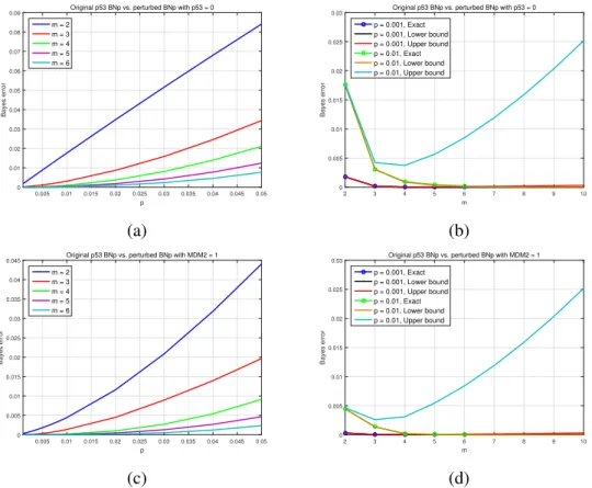
(per-turbed) BNp with MDM2 = 1. Reprinted with permission from [1], c2018 IEEE. . . 31 2.6 (a) and (b): Bayes error versuspandm. First class is the wild-type p53 BNp, and the second is

mutated BNp with deactivated gene p53. (c) and (d): Bayes error versuspandm. First class is the wild-type p53 BNp, and the second is mutated BNp with activated gene MDM2. Reprinted with permission from [1], c2018 IEEE.. . . 32 2.7 Mammalian cell-cycle gene regulatory network. Reprinted with permission from [1], c2018 IEEE.. 33 2.8 Lower and upper bounds of the Bayes error versus m. The two classes are the wild-type and

mutated (with p27 = 0) mammalian cell-cycle PBNs. Reprinted with permission from [1], c2018 IEEE.. . . 34 2.9 Factor graph of the HMM. Reprinted with permission from [2], c2019 IEEE.. . . 50 2.10 Classification error of single-cell trajectory method versusm. The classification error of the

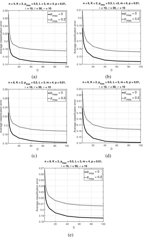
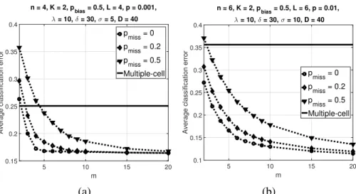
multiple-cell averaging method is also included in the plots for comparison. Reprinted with permission from [2], c2019 IEEE. . . 63 2.11 Average classification error of the trajectory classifier over500synthetic BNs versusDwithK= 2

andpbias = 0.5. Parameter values arep= 0.01,λ = 10,δ = 30,σ = 10, (a)n = 4,L = 3,

m= 4, (b)n= 4,L= 5,m= 6, (c)n= 6,L= 3,m= 4, (d)n= 6,L= 5,m= 6, (e)n= 8,

(12)

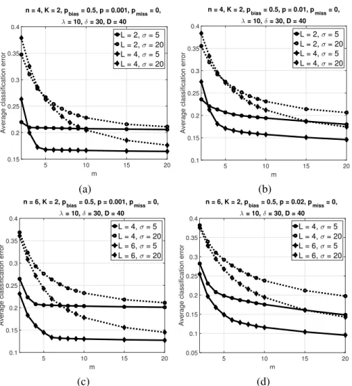
2.12 Average classification error of the trajectory classifier over500synthetic BNs versusmwithK= 2 andpbias= 0.5. Parameter values arepmiss= 0,λ= 10,δ= 30,D= 40, (a)n= 4,p= 0.001,

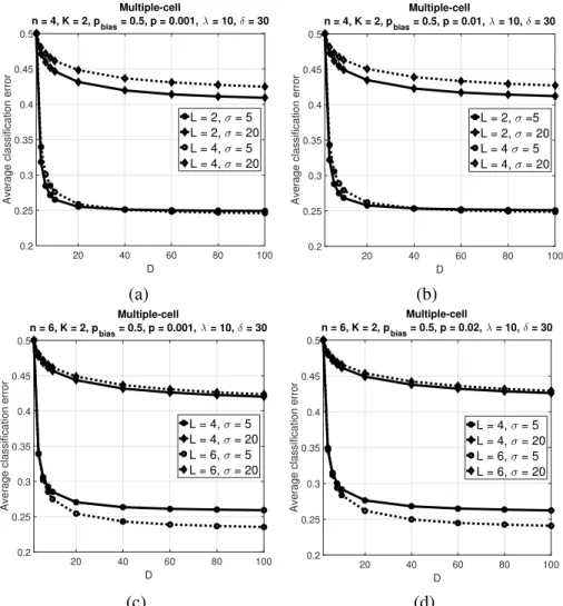
(b)n = 4,p = 0.01, (c)n = 6,p = 0.001, (d)n = 6,p = 0.02. Reprinted with permission from [2], c2019 IEEE. . . 66 2.13 Average classification error of the multiple-cell classifier over500 synthetic BNs versusD with

K = 2andpbias = 0.5. Parameter values areλ= 10,δ= 30, (a)n= 4,p= 0.001, (b)n= 4,

p= 0.01, (c)n= 6,p= 0.001, (d)n= 6,p= 0.02. Reprinted with permission from [2], c2019 IEEE.. . . 67 2.14 Average classification error of the trajectory classifier and multiple-cell classifier over500synthetic

BNs versusmwithK = 2andpbias = 0.5. Parameter values areλ= 10,δ = 30,D = 40, (a)

n= 4,L= 4,p= 0.001,σ= 5, (b)n= 6,L= 6,p= 0.01,σ= 10. Reprinted with permission from [2], c2019 IEEE. . . 68 2.15 Mammalian cell-cycle gene regulatory network. Reprinted with permission from [2], c2019 IEEE.. 70 2.16 Classification errors of the trajectory and multiple-cell classifiers in the mammalian cell-cycle BN.

The fixed parameters aren= 10,λ= 10,δ= 30. (a) Classification error of the trajectory classifier versusD. The parameters arem = 6,p= 0.05,σ = 5, (b) Classification error of the trajectory classifier versusD. The parameters arem = 6,p= 0.05,σ = 20, (c) Classification error of the multiple-cell classifier versusD. The parameter isp= 0.01, (d) Classification error of the multiple-cell classifier versusD. The parameter isp= 0.05, (e) Classification error of the trajectory and multiple-cell classifiers versusm. The parameters areD= 40,p= 0.05,σ= 5, (f) Classification error of the trajectory and multiple-cell classifiers versusm. The parameters areD= 40,p= 0.05,

σ= 20. Reprinted with permission from [2], c2019 IEEE.. . . 71 2.17 Classifier error versusmin cell-cycle network. Reprinted with permission from [3], c2018 BMC.. . 85 2.18 Classifier error versusmin cell-cycle network. Reprinted with permission from [3], c2018 BMC.. . 85 2.19 Classifier error versusα0in cell-cycle network. Reprinted with permission from [3], c2018 BMC. . 86 2.20 Classifier error versusβ0in cell-cycle network. Reprinted with permission from [3], c2018 BMC.. . 86 2.21 Classifier error versusain cell-cycle network. Reprinted with permission from [3], c2018 BMC.. . . 87 2.22 Classifier error versusbin cell-cycle network. Reprinted with permission from [3], c2018 BMC.. . . 88 2.23 Classifier error versusκ0in cell-cycle network. Reprinted with permission from [3], c2018 BMC.. . 88 2.24 Classifier error versusδ0in cell-cycle network. Reprinted with permission from [3], c2018 BMC.. . 89 3.1 Dependency of the source and target domains through their precision matrices for any classl ∈

(13)

3.2 (a) Average classification error versus the number of target training data per class,nt, (b)

Aver-age classification error versus the number of source training data per class, ns. Reprinted with

permission from [4], c2018 IEEE.. . . 109

3.3 Box plots of1000simulated classification errors for differentnt. Blue denotes the OBC and red denotes the OBTL withα= 0.9. Reprinted with permission from [4], c2018 IEEE.. . . 110

3.4 Average classification error vs|α|. Reprinted with permission from [4], c2018 IEEE.. . . 111

3.5 Average classification error vsν. Reprinted with permission from [4], c2018 IEEE.. . . 112

3.6 Average classification error vsκt. Reprinted with permission from [4], c2018 IEEE. . . 113

3.7 Accuracy in theOffice+Caltech256dataset versus: (a)ktwhen ks = 1/200 and for two experi-mentsa→w, α= 0.6andw→d, α= 0.99, (b)kswhenkt = 1/200and for two experiments a → w, α = 0.6 andw → d, α = 0.99, (c) αwhen kt = ks = 1/200and for the experiment a→w, (d)αwhenkt =ks= 1/200and for the experimentw→d. Reprinted with permission from [4], c2018 IEEE. . . 116

3.8 Average MSE versusntfor the two cases, assumingns= 500. Reprinted with permission from [5], c 2018 IEEE.. . . 127

3.9 Average MSE versusnsfor the two cases, assumingnt= 5. Reprinted with permission from [5], c 2018 IEEE.. . . 127

3.10 Dependency of the source and target domains through their mean and shape parameters for any genei∈ {1,· · ·, d}and classl∈ {1,· · · , L}. Reprinted with permission from [6], c2019 IEEE. . . 138

3.11 Average classification error versus the number of target training dataNtand the number of source training dataNs. Reprinted with permission from [6], c2019 IEEE.. . . 145

3.12 Average classification error versusρrandρµused in the OBTL classifier. The true data generating values are written on top of each figure. Reprinted with permission from [6], c2019 IEEE.. . . 147

3.13 RNA-Seq counts of ten genes in two domains and for two classes LUAD and LUSC from TCGA. Red denotes the target domain, which is RNA-Seq data from TCGA. Blue denotes the source do-main, which is RNA-Seq-v2 from TCGA. We see that the source domain has lower values than the target domain. (a) First feature set with the following ten genes (ordered from 1 to 10 suc-cessively): USP31, FGF11, CLCF1, C15orf41, KLF2, TMEM79, CD302, SDHAP3, TSPAN12, CABLES1, (b) Second feature set with the following ordered genes (ordered from 1 to 10 succes-sively): ACBD4, DTL, DISP1, BUB1B, MTMR11, CHAF1A, C9orf7, SIGIRR, C1orf74, GEN1. Reprinted with permission from [6], c2019 IEEE.. . . 148

(14)

3.14 RNA-Seq counts of ten genes in two domains and for two classes KIRP and KIRC from TCGA. Red denotes the target domain, which is RNA-Seq-v2 data from TCGA. Blue denotes the source domain, which is RNA-Seq from TCGA. We see that the source domain has larger values than the target domain. (a) Kidney feature set with the following ten genes (ordered from 1 to 10 succes-sively): MCC, PTP4A3, ABHD14B, VPS25, C9orf116, LEPREL1, NOSTRIN, GTF2IRD1, GEM, MMP24. Reprinted with permission from [6], c2019 IEEE.. . . 149 B.1 Exact values of function 2F1(a, b;c;τ Id)and its Laplace approximation 2Fˆ1(a, b;c;τ Id)versus:

(a)τ, ford = 5,a = 3,b = 4, andc = 6, (b)c, ford= 10,a = 30,b = 50, andτ = 0.01. Reprinted with permission from [4], c2018 IEEE.. . . 180

(15)

LIST OF TABLES

TABLE Page

2.1 (a) Truth table of the original and mutated Boolean functionsf and˜f, (b) The Bayes error for all the 1-bit function perturbations.m= 4andp= 0.01. Reprinted with permission from [1], c2018 IEEE.. . . 26 2.2 Definitions of Boolean functions in wild-type p53 BNp. Reprinted with permission from [1],

c

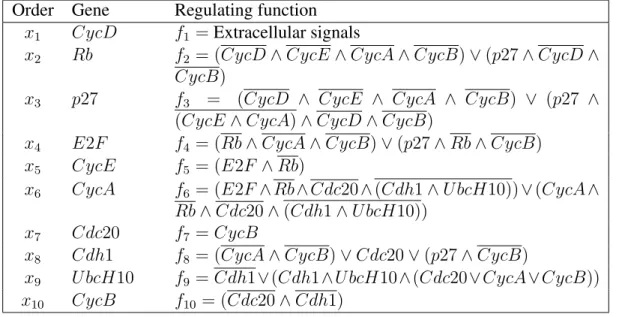
2018 IEEE.. . . 31 2.3 Definitions of Boolean functions for the wild-type mammalian cell-cycle PBN with 10 genes.

Reprinted with permission from [1], c2018 IEEE.. . . 34 2.4 Definitions of Boolean functions for the wild-type mammalian cell-cycle BN with10genes. Reprinted

with permission from [2], c2019 IEEE.. . . 70 3.1 Semi-supervised accuracy for different source and target domains in theOffice+Caltech256dataset

using SURF features. Domain names are denoted as a:amazon, w:webcam, d:dslr, c:Caltech256. The numbers in red show the best accuracy and the numbers in blue show the second best accuracy in each column. The results of the first six methods have been adopted from [8]. Similar to [8], we have also used the evaluation setup of [9] for the OBTL. Reprinted with permission from [4],

c

2018 IEEE.. . . 115 3.2 The values of hyperparameterαof the OBTL used in each experiment.ntandnsare based on the

data splits provided by [9]. Reprinted with permission from [4], c2018 IEEE.. . . 115 3.3 Average RMS errors on five UCI datasets, each divided into three cases as in [10]. In each case,

target and source data are different. Bold font marks the lowest error for the OBR and OBTR with different values ofτ. In each case,nt = 10andns = 200. C 1 means Case 1. Reprinted with

permission from [5], c2018 IEEE.. . . 129 3.4 The average error of the OBTL classifier using the first feature set in the TCGA data for the

clas-sification of LUAD and LUAC assuming different values ofρµandρr. The corresponding average

error for the OBC is0.1312. The minimum error is written in bold. Reprinted with permission from [6], c2019 IEEE. . . 150 3.5 The average error of the OBTL classifier using the second feature set in the TCGA data for the

clas-sification of LUAD and LUAC assuming different values ofρµandρr. The corresponding average

error for the OBC is0.1776. The minimum error is written in bold. Reprinted with permission from [6], c2019 IEEE. . . 151

(16)

3.6 The average error of the OBTL classifier using the kidney feature set in the TCGA data for the clas-sification of KIRP and KIRC assuming different values ofρµandρr. The corresponding average

error for the OBC is0.0866. The minimum error is written in bold. Reprinted with permission from [6], c2019 IEEE. . . 152

(17)

1. INTRODUCTION

Machine learning has become one of the most important and challenging research topics today with immense number of applications such as genomics or computer vision, which owes its pop-ularity to the emergence of different types of data which can now be easily acquired thanks to the growth of technology. Being exposed to different types of data coming from various measurement technologies lead to great amount of heterogeneity in data, which had not been experienced so far. As a result, we would more likely be very far away from the identically and independently distributed (i.i.d.) assumption, upon which many machine learning methods have been built. In this dissertation, we have addressed two types of heterogeneity in data: heterogeneity due to time evolution and heterogeneity due to domain difference. First, we address the time heterogeneity via modeling the dynamics of data. Second, we solve heterogeneity due to domain difference via transfer learning.

In chapter 2, we thoroughly study the classification of gene expression trajectories using the partial knowledge of gene regulatory networks (GRN). Traditionally, gene expression data from different sources of measurements, such as microarray and RNA-Seq, have been used for phe-notype classification, that is, the classification of cancer versus normal or the classification of different types of diseases. According to the fact that the genes in our cells interact with each other and actually evolve over time via a GRN, we propose to model their dynamics and classify phenotypes using gene expression trajectories (time-series) which contain more information than the static data which are a snapshot of gene expressions in one time point. We first use partially known GRNs and model the gene expression state trajectories using Boolean Networks with per-turbation (BNp), where a gene has two values: 1 for On and 0 for Off. We study the classification error under different mutated networks and attractor cycles and show that the mutations which change the attractor structures more lead to lower classification error. We then generalize it to real gene expression trajectories by assuming an observation model on top of state dynamics. Thanks to recent single-cell sequencing technologies, we are now able to sequence the gene expressions

(18)

inside every cell at each time point and generate meaningful gene expression trajectory data which can reflect the dynamics of gene regulatory networks. We design a classifier using single-cell gene expression trajectories and show that it can significantly outperform the classifiers which use static gene expression data derived from bulk gene expression technologies like RNA-Seq. The reason is that in bulk RNA-Seq, the expression values of genes are averaged over the population of cells and the dynamics cannot be captured. For the single-cell gene expression trajectories, we propose an expectation maximization (EM) algorithm with closed-from updates which can efficiently esti-mate the unknown parameters of the model using the observed trajectories. We finally study the single-cell gene expression trajectories in a Bayesian framework and propose intrinsically Bayesian robust classifier for the trajectories, where instead of estimating the unknown parameters, we as-sume they belong to an uncertainty class governed by a prior distribution. We evaluate all these methods on different important gene regulatory networks including p53 and cell cycle networks and demonstrate their efficacy in accurately classifying different phenotypes.

In chapter 3, we study transfer learning with a novel Bayesian viewpoint. Transfer learning appears where we do not have enough data in our target domain to train the machine learning algorithms well but have good amount of data in other relevant source domains. The probabil-ity distributions of the source and target domains might be totally different but they share some knowledge underlying the similar tasks between the domains and are related to each other in some sense. The ultimate goal of transfer learning is to find the amount of relatedness between the do-mains and then transfer the amount of knowledge to the target domain which can help improve the classification task in the data-poor target domain. Domain adaptation (DA) is a method to address transfer learning, where the source and target data are mapped to a common domain in which they follow a similar distribution. However, domain adaptation is not a very clever way of addressing transfer learning in that it can only work well when the two domains are highly related and can easily fail if there are huge distribution difference between the source and target domains. Indeed, many existing transfer learning and domain adaptation methods fail to answer questions regarding the relatedness and transferability between the source and target domains. As a result, they are very

(19)

prone tonegative transfer, which is a phenomenon in which transfer learning fails to transfer help-ful knowledge to the target domain and consequently deteriorates the performance compared to the target-only training without transferring any knowledge. Negative transfer is the most vital issue in transfer learning and happens when the algorithm is not able to detect that the source domain is not related to the target domain for a specific task. For solving all these issues, we propose a novel transfer learning method based on a Bayesian framework, which is the scope of chapter 3. We propose a Bayesian transfer learning framework, where the source and target domains are related through the joint prior distribution of the model parameters. The modeling of joint prior densities enables better understanding of the transferability between domains. We first consider continuous data under a Gaussian model. We define a joint Wishart distribution for the precision matrices of the Gaussian feature-label distributions in the source and target domains to act like a bridge that transfers the useful information of the source domain to help classification in the target domain by improving the target posteriors. Using several theorems from multivariate statistics, the posteriors and posterior predictive densities are derived in closed forms in terms of hypergeometric functions of matrix argument, leading to our novel closed-form and fast Optimal Bayesian Transfer Learning (OBTL) classifier. Then we generalize the OBTL for the regression problem and similarly propose Optimal Bayesian Transfer Regression (OBTR). Finally, we extend our transfer learning idea to count data with the aim of cancer classification using the next generation sequencing data such as RNA-Seq. In this case, for addressing over-dispersion in RNA-Seq data, we use Negative Bino-mial (NB) and define joint priors for the parameters of the source and target domain. We learn the posteriors using Hamiltonian Monte Carlo (HMC) algorithm and then define the optimal transfer learning classifier for the count data. We evaluate the performance of our proposed transfer learn-ing methods for classification and regression uslearn-ing both image and cancer datasets and show that they are able to optimally transfer the relevant knowledge from the source to the target domain and consequently improve the performance of data-poor target domains.

(20)

2. CLASSIFICATION OF GENE EXPRESSION TRAJECTORIES USING THE KNOWLEDGE OF GENE REGULATORY NETWORKS∗

2.1 Classification of Gene State Trajectories 2.1.1 Overview

Gene-expression-based phenotype classification is used for disease diagnosis and prognosis relating to treatment strategies. In this section we study classification based on sequential mea-surements of multiple genes using gene regulatory network (GRN) modeling. We assume there are two networks, original (healthy) and mutated (cancerous), and observations consist of trajectories of network states. The problem is to classify an observation trajectory as coming from either the original or mutated network. GRNs are modeled via probabilistic Boolean networks (PBN), which incorporate stochasticity at both the gene and network levels. Mutation affects the regulatory logic. Classification is based upon observing a trajectory of states of some given length. We characterize the Bayes classifier and find the Bayes error for a general PBN and the special case of a single Boolean network affected by random perturbations (BNp). The Bayes error is related to network sensitivity, meaning the extent of alteration in the steady-state distribution of the original network owing to mutation. Using standard methods to calculate steady-state distributions is cumbersome and sometimes impossible, so we provide an efficient algorithm and approximations. Extensive simulations are performed to study the effects of various factors, including approximation accu-racy. We apply the classification procedure to a p53 BNp and a mammalian cell cycle PBN.

∗_{Reprinted with permission from “Classification of Single-Cell Gene Expression Trajectories from Incomplete and}

∗_{Reprinted with permission from “Intrinsically Bayesian robust classifier for single-cell gene expression}

∗_{Reprinted with permission from “Classification of State Trajectories in Gene Regulatory Networks” by A.}

(21)

2.1.2 Introduction

Gene-expression-based phenotype classification was among the first applications proposed for high-throughput expression measurements, starting with DNA microarrays, the aim being disease diagnosis or prognosis relating to treatment strategies [11-14]. Owing to feature selection and error estimation in extremely high-dimensional spaces with limited sample data, accurate classification and error estimation have proven to be difficult, even with the advent of RNA-seq data [15-20]. Measurement noise in high-throughput data and heterogeneity across samples and patients increase the challenge. One proposed approach is to use groups of genes as features, such as merging genes in signaling pathways. This can help avoid redundant information contained in selected genes, for instance, selecting several genes in a pathway that are regulated by a single master gene [21]. The approach is to jointly analyze the expression levels of genes related by functionality, which can be obtained via transcriptome analysis [22-24], GO annotations [25], or other sources. Several methods have been proposed to measure the activity of a particular pathway: mean or median [26], first principle component [24], using a subset of genes in the pathway [27], and combining log-likelihood ratios of genes in the pathway [28].

While the aforementioned methods take advantage of multiple gene activity, in the end they all rely on single measurements and therefore do not take advantage of the regulatory information in trajectory data. In this section we consider classification based on sequential measurements of multiple genes. The problem is modeled via gene regulatory networks (GRNs). There are two networks, an original and one having undergone mutation, and observations consist of trajectories of network states, the classification problem being to classify an observation trajectory as coming from either the original or mutated network.

Before describing the mathematical setting, we note that traditionally it has been difficult to collect time-course gene-expression data for cancer, not only because cancer is known for its het-erogeneity, but also because the cells are not synchronized. Thus, traditionally, for quality time-course expression data, one has to purify and synchronize the whole cell population, which is very challenging and cannot be achieved in a routine manner [29]. However, with the breakthrough in

(22)

single-cell profiling, the problem can be overcome by profiling individual cells using RNA-Seq or quantitative PCR [30]. The individual cells can be captured via standard methods, such as flow cytometry, glass capillaries, or laser [31], and be measured at various time points. For example, in [32], between49to77cells have been collected at each time for4total time points and a soft-ware, Monocle, has been built to extract various gene-expression trajectories of individual cells. The authors have shown that key gene-expression transition sequences can be observed based on the trajectories. The method, according to the authors, can also be applied to time-course data col-lected via quantitative PCR. Since the regulation dynamic can provide a wide range of information not readily available from existing medical tests, driven by the need for personalized treatment, one would envision that in the future such procedures might be commercialized to help physicians make better diagnoses and choose the best treatments.

We model GRNs via probabilistic Boolean networks (PBNs) [33]. These characterize regula-tory relations over discrete steps, which need not be time but instead can be related to gene state transitions such as in the cell cycle. They incorporate stochasticity at the gene level by allowing random gene perturbation and at the network level by consisting of multiple Boolean networks randomly selected based upon the activity of latent variables outside the network. While for sim-plicity we assume binary values, corresponding to a gene expressing or not expressing, the general PBN model makes no such assumption and the results of this work extend directly to multi-valued genes. PBNs have been used extensively for the study of optimal intervention based on control over time [34] and a one-time targeted alteration of the regulatory functions [35].

We assume that the mutated network has arisen from a mutation affecting the regulatory logic, and classification is based upon observing a trajectory of states of some given length. In this section, we characterize the Bayes classifier and find the Bayes error for a general PBN and the special case of a single Boolean network (BNp) affected by random perturbations. It will be seen that longer trajectories lower the Bayes error. We also see that if the two networks are similar and share some same attractor cycles, the longer trajectories are required to achieve a desired Bayes error close to zero, but when they are totally dissimilar, even the short trajectories can result in a

(23)

lower Bayes error. As is commonly assumed (although not always mentioned), we suppose that classification is in the steady-state. Owing to perturbation, the Markov chain corresponding to a PBN is irreducible and hence possesses a steady-state distribution for the states.

We relate the Bayes error to the sensitivity of the network to mutation, where by sensitivity we mean quantification of the alteration in the steady-state distribution of the original network owing to mutation [36]. We define a trajectory-based notion of sensitivity suitable to the classification problem. Lack of sensitivity is good for cell survival because long-run wild-type state probabilities are not significantly altered, but this makes classification more difficult. If a function mutation significantly reduces the number of common attractor states in the two networks, then the Bayes error will be low. However, if the function mutation does not change the attractor structures of the original network, we cannot expect to have a Bayes error around zero, unless we have access to very long trajectories. The steady-state probabilities of attractors in PBNs have been derived in [37] with good approximations.

Using standard methods to calculate steady-state distributions is cumbersome and sometimes impossible due to the high computation time required for inverting large transition probability matrices (TPMs). We provide an efficient algorithm to help ease the computation; nevertheless, the computational burden is still prohibitive when the trajectory length is long, especially because we want to do simulations over large numbers of networks. Therefore, we provide approximations when the gene perturbation probability is small, a common assumption. We provide extensive simulations to study the effects of various factors, including the goodness of the approximations. Finally we apply the classification procedure to a p53 BNp and a mammalian cell cycle PBN.

2.1.3 Background

For a binary Boolean network (BN) onngenes, a truth table gives the functional relationships between the genes [38]. Each gene valuexi ∈ {0,1}, fori= 1,· · · , n, at timek+ 1is determined

by the values of some predictor genes at timekvia a Boolean functionfi :{0,1}n→ {0,1}in the

truth table. In practice,fi is a function of small number of genes,Ki, which is called input degree

(24)

with vertices representing genes and edges representing regulations. Given an initial state, a BN will eventually reach a set of states, called anattractor cycle, through which it will cycle endlessly. Each initial state corresponds to a unique attractor cycle, and the set of initial states leading to a specific attractor cycle is known as thebasin of attraction(BOA) of the attractor cycle.

2.1.3.1 Boolean Networks with perturbation (BNp)

For BNps, perturbation is introduced with a probability p by which the current state of the network can be randomly changed. Implicitly, we assume that there is an independent identically distributed (i.i.d.) random perturbation vector at each timek, denoted bynk ∈ {0,1}n, where the

ith gene flips at timekif theith component ofnkis equal to1. Therefore, the dynamical model of

the states can be expressed as

xk+1 =f(xk)⊕nk+1, k = 0,1,2,· · · , (2.1)

where xk = [x1(k), x2(k),· · ·, xn(k)]T is a binary state vector, called a gene activity profile

(GAP), at time k, in which xi(k) indicates the expression level of the ith gene at time k (either

0 or 1); f(xk) = [f1, f2,· · · , fn]T : {0,1}n → {0,1}n is the vector of the network functions,

in which fi shows the expression level of the ith gene at time k + 1 when the system lies in

the state xk at time k; nk = [n1(k), n2(k),· · ·, nn(k)]T is the perturbation vector at timek, in

whichn1(k), n2(k),· · · , nn(k)are i.i.d. Bernoulli random variables for everyk with the

parame-terp=P(ni(k) = 1); and⊕is component-wise modulo2addition. The existence of perturbation

makes the corresponding Markov chain of a BNp irreducible. Hence, the network possesses a steady-state distributionπdescribing its long-run behavior. A BNp inherits the attractor structure from the original BN without perturbation, the difference being that a random perturbation can cause a BNp to jump out of an attractor cycle, perhaps then transitioning to a different attractor cycle. Ifpis sufficiently small,πwill reflect the attractor structure within the original network. We can derive the transition probability matrix (TPM) if we know the truth table and the perturbation probability for a BNp. As a result, the steady-state distributionπcan be computed as well.

(25)

2.1.3.2 Probabilistic Boolean Network (PBN)

The network function in a PBN is not fixed and changes over time. We first consider

context-sensitivePBNs, in which the current function governing the network will be changed if a switchξis

on (ξ = 1), which has the probabilityq. When the switch is on, the new network function will be se-lected amongL functions{f(1),f(2),· · · ,f(L)} with corresponding probabilities{c1, c2,· · · , cL}.

Then we analyze instantaneously random PBNs, which are a special case of context-sensitive PBNs with q = 1, meaning that the network functions are changing at each time point indepen-dently with the selection probabilities{c1, c2,· · · , cL}. The PBN dynamics are defined as

xk+1 =fk+1(xk)⊕nk+1, k = 0,1,2,· · ·, (2.2)

wherexk and nk denote the state and perturbation vectors, as defined in (2.1). Here, fk+1 is the

network function at timek+1, which is randomly picked from the context set{f(1)_,_f(2)_,_{· · ·}_,_f(L)_},

with the aforementioned probabilities, at each time k + 1. A BNp is a PBN possessing a single context, that is,L= 1. WhenL= 1,fk+1 =f(1)in (2.2) is a constant function over time and (2.2)

turns to the BNp definition in (2.1).

In this section, we address the following problem. Suppose the truth table governing the orig-inal BNp (or PBN) is altered to yield amutated BNp (PBN), keepingp unchanged, and we are given an observed trajectory of the states in the steady-state. Our goal is to classify this arbitrary trajectory as belonging to the original or mutated BNp (PBN). We will obtain the Bayes classifier for this problem and find the corresponding Bayes error for the classifier.

2.1.4 Methods

2.1.4.1 Bayes Classifier

•Context-sensitive PBN:

We first consider the general case of context-sensitive PBNs. Let xk denote an n×1binary

state vector at timek. Letx¯k = 1 +

Pn

(26)

¯

xk∈ {1,2,· · ·,2n}; for instance,(0,0, ...,0)T →1and(1,1, ...,1)T →2n. In a context-sensitive

PBN the state of the corresponding Markov chain at each time consists of both a GAP and a context, and is of the form(Xk,Fk). Thus, the TPM has dimension2n×Lby2n×L. Its entries are the

probabilitiesP(Xk+1 =xk+1,Fk+1 =fk+1|Xk =xk,Fk = fk). In our classification problem we

only have access to the GAP observations in the steady-state. As a result, we will use a hidden Markov model (HMM) to compute the probability of a given GAP trajectory in the steady-state.

The TPM in this case is a2n×Lby2n×Lmatrix, whose entries are defined by

P(Xk+1 =xk+1,fk+1 =f(i)|Xk =xk,fk =f(j)) = P(Xk+1 =xk+1|Xk=xk,fk+1 =f(i)) ×P(fk+1 =f(i)|fk =f(j)). (2.3) From (2.2) we have P(Xk+1 =xk+1|Xk=xk,fk+1 =f(i)) = pd(xk+1,f(i)(xk))₍₁₋_p)n−d(xk+1,f(i)(xk))_, _(2.4)

where d(xk+1,f(i)(xk)) is the Hamming distance between two binary vectorsxk+1 and f(i)(xk).

We know that{fk}itself forms an irreducible Markov chain, and consequently possesses a

steady-state distribution. If the current function isf(i), then the probability that the function stays fixed at the next time is1−q+qci,which is the addition of the probabilities of two exclusive events:

the network switch is not called for (probability1−q), or the switch is called for and the current network is selected again (probabilityqci). If the current function is notf(i), then the probability

thatf(i)_{will be the network function at the next time point is}_qc

i, which is the probability that the

switch is called for and the functionf(i)_{is selected. Therefore, we can write,}

(27)

fori, j = 1,· · · , L. Consequently, from (2.3)-(2.5), the TPM has the following entries,

P(Xk+1 =xk+1,fk+1 =f(i)|Xk =xk,fk =f(j)) =

{1[i=j](1−q+qci) + 1[i6=j](qci)}

×pd(xk+1,f(i)(xk))₍₁₋_p)n−d(xk+1,f(i)(xk))_. _(2.6)

Now we aim to compute the probability of a given GAP trajectory in a specific PBN in the steady-state. Suppose X = [xs,xs+1,· · · ,xs+m−1] is an observed trajectory of length m in the

steady-state, wheresis a time point in the steady-state, andF = [fs+1,· · · ,fs+m−1]is composed

of the hidden network functions from times+ 1tos+m−1. The joint probability ofX andF is

P(X,F) = P(X |F)P(F), (2.7)

whereP(X |F)andP(F)can be factorized as

P(X |F) = P(xs) m−1 Y k=1 P(xs+k|xs+k−1,fs+k) (2.8) P(F) = P(fs+1) m−1 Y k=2 P(fs+k|fs+k−1). (2.9)

In order to derive the probability of trajectory,P(X), we should marginalize the joint PMF of (2.7) overF,

P(X) = X

F

P(X,F), (2.10)

which can be efficiently computed using the forward update in the structure of the HMM due to the factorization in (2.8) and (2.9). We define the vectorsαk, fork =s+ 1,· · · , s+m−1, with

(28)

αs+1(i) = P(xs)P(fs+1 =f(i))P(xs+1|xs,fs+1=f(i)), αs+k+1(i) =P(xs+k+1|xs+k,fs+k+1 =f(i)) × L X j=1 αs+k(j)P(fs+k+1 =f(i)|fs+k =f(j)), (2.11) wherek = 1,· · · , m−2andi= 1,· · · , L.

Proposition 1: The steady-state distribution of the network functions is equal to their selection probabilities, that is,P(fk=f(i)) =ci, wherek → ∞.

Proof: From the total probability rule,

P(fk+1 =f(i)) =P(fk+1 =f(i)|fk=f(i))P(fk =f(i))

+P(fk+1 =f(i)|fk6=f(i))P(fk6=f(i)). (2.12)

As mentioned before,{fk}is an irreducible Markov chain and has a steady-state distribution, that

is, P(fk+1 = f(i)) = P(fk = f(i))whenk → ∞; using this and (2.5) in (2.12) leads toP(fk =

f(i)_{) =}_c

i, wherek→ ∞.

According to Proposition 1,P(fs+1 =f(i)) =ciin (2.11). Furthermore,P(xs) = π¯xs in (2.11)

is the steady-state distribution ofxs, which can be computed from the TPM in (2.6). Hence, we

can rewrite (2.11) as αs+1(i) =πx¯sciP(xs+1|xs,fs+1 =f (i) ), αs+k+1(i) =P(xs+k+1|xs+k,fs+k+1 =f(i)) × L X j=1 αs+k(j)P(fs+k+1 =f(i)|fs+k=f(j)). (2.13)

(29)

can be computed by summing the entries ofαs+m−1as P(X) = L X i=1 αs+m−1(i). (2.14)

Supposeπx¯s andπ˜x¯s are the steady-state probabilities of being in state xs in the original and

mutated PBNs, respectively, {f(1)_,_{· · ·} _,_f(L)_} _and _{_˜_f(1)_,_{· · ·} _,_˜_f(L)_} _{are the} _L _{constituent network}

functions of the original and mutated PBNs, respectively, and{c1, c2,· · · , cL}and{˜c1,˜c2,· · · ,˜cL}

are the corresponding function selection probabilities. As a result, the probability of the trajectory X in the original network,P(X |P BNoriginal), can be computed from (2.14). We can also compute

the probability of the trajectory X in the mutated network, P(X |P BNmutated), using (2.14), but

we should useπ˜x¯s,˜f

(i)_,_c_˜

i, andq˜instead ofπx¯s,f

(i)_,_c

iandq, respectively, in (2.1)-(2.14).

Let p0 andp1 be the prior probabilities of the original and mutated PBNs, respectively. Then

the posterior probabilities of the classes after observing the trajectoryX are

η(X) = P(P BNmut.|X) = p1P(X |P BNmut.) P(X) , (2.15) 1−η(X) =P(P BNorig.|X) = p0P(X |P BNorig.) P(X) . (2.16)

The Bayes classifier is given by

ψ?(X) =      1, η(X)≥1−η(X) 0, η(X)<1−η(X) =      1, p1P(X |P BNmut.)≥p0P(X |P BNorig.) 0, p1P(X |P BNmut.)< p0P(X |P BNorig.) . (2.17)

In (2.17), the classes0 and1denote the original and mutated PBNs, respectively. If we assume the classes are equally likely, p0 = p1 = 1₂, thenp0 andp1 can be dropped from both sides of the

(30)

•Instantaneously random PBN:

Now we consider the caseq= 1, which means that the network functions are changing at each time point. The probability of selectingf(i) _{at time}_k_{+ 1}_{is independent of the previous network}

function at timekand is equal toci. We can see this fact from (2.5):

P(fk+1 =f(i)|fk =f(j)) = P(fk+1 =f(i)) =ci. (2.18)

Furthermore, the TPM in (2.6) becomes

P(Xk+1 =xk+1,fk+1 =f(i)|Xk =xk,fk =f(j)) =

cipd(xk+1,f

(i)₍_x

k))₍₁₋_p)n−d(xk+1,f(i)(xk))

=P(Xk+1 =xk+1,fk+1 =f(i)|Xk =xk). (2.19)

As a result, the TPM of the GAP can be achieved by marginalizing (2.19) overf(i)_as

P(Xk+1 =xk+1|Xk =xk) = L X i=1 cipd(xk+1,f (i)₍_x k))₍₁₋_p)n−d(xk+1,f(i)(xk))_. _(2.20)

Note that in this case,P(F)in (2.9) is factorized as (based on independence)

P(F) =

m−1 Y

k=1

P(fs+k). (2.21)

From (2.7), (2.8), (2.10), and (2.21), we have

P(X) =πx¯s

m−2 Y

k=0

P(Xs+k+1 =xs+k+1|Xs+k =xs+k). (2.22)

(31)

original and mutated instantaneously random PBNs are P(X |P BNoriginal) =πx¯s m−2 Y k=0 ( _L X i=1 cipd(xs+k+1,f (i)₍_x s+k))₍₁₋_p)n−d(xs+k+1,f(i)(xs+k)) ) , (2.23) P(X |P BNmutated) = ˜π¯xs m−2 Y k=0 ( _L X i=1 ˜ cipd(xs+k+1, ˜ f(i)₍_x s+k))₍₁₋_p)n−d(xs+k+1,˜f(i)(xs+k)) ) . (2.24)

The Bayes classifier is the same as in (2.17). •BNp:

According to (2.1), the TPM of a BNp is a2n_×₂n_{matrix with the following entries.}

P(Xk+1 =xk+1|Xk =xk) =pd(xk+1,f(xk))(1−p)n−d(xk+1,f(xk)). (2.25)

We can see that the TPM in (2.25) can also be achieved from the TPM of the GAP in the instan-taneously random PBN (2.20) by lettingL = 1, c1 = 1, andf(1) =f. The probability ofX in the

BNp is P(X) =πx¯s m−2 Y k=0 P(Xs+k+1 =xs+k+1|Xs+k =xs+k). (2.26)

Using (2.25) and (2.26), the probability ofX in the original and mutated BNps can be written as

P(X |BN poriginal) =πx¯sp Pm−2 k=0 d(xs+k+1,f(xs+k)) ×(1−p)n(m−1)−Pmk=0−2d(xs+k+1,f(xs+k))_, _(2.27) P(X |BN pmutated) = ˜πx¯sp Pm−2 k=0 d(xs+k+1,˜f(xs+k)) ×(1−p)n(m−1)−Pmk=0−2d(xs+k+1,˜f(xs+k))_, _(2.28)

(32)

(2.17), the Bayes classifier is ψ?(X) =      1, p1P(X |BN pmut.)≥p0P(X |BN porig.) 0, p1P(X |BN pmut.)< p0P(X |BN porig.) , (2.29)

where the classes0and1denote the original and mutated BNps, respectively.

The GAP steady-state distributionπ = [π1, π2,· · · , π2n]can be easily calculated using the fact

thatπ = πP andP2_i₌₁n πi = 1, whereP is the GAP TPM of the original instantaneously random

PBN and original BNp, whose entries are respectively computed using (2.20) and (2.25). More specifically,π =πP can be written in the formπ(I −P) = 0. We knowI −P is not a full-rank matrix and that one out of 2n_{linear equations depends on the others. Therefore, we remove one}

column (say the last column) of the matrixI−P and replace it by an all-one column, which adds the normalization constraint,P2_i₌₁n πi = 1, to the set of the linear equations π = πP. Calling the

resultant matrixQ, we have

π = [0,0,· · · ,0,1]Q−1. (2.30) We know from the Markov chain properties that Qis a full-rank matrix and has an inverse. We should also note that although computing the steady-state distribution using (2.30) is exact, it may not be the most efficient method in terms of the computation time. As a result, we may need to use the approximate and faster algorithms, like power methods, to computeπ in very large networks. For the mutated PBN,π˜ can be similarly derived. However, as we will study the behavior of the average Bayes error over many random networks and many random mutations, we will provide an algorithm to computeπ˜very efficiently without a need for matrix inversion like in (2.30).

2.1.4.2 Bayes Error and Long-run Sensitivity

This section provides the Bayes error for the previously derived Bayes classifiers. It uses the fact that the Bayes error can be expressed via the posterior probabilities by

(33)

•Bayes error for BNps:

From (2.15), (2.16) (replacing PBNs with BNps), and (2.31), and with the assumption of equally likely BNps, i. e.,p0 =p1 = 1₂, the Bayes error can be written as

? = 1 2

X

min{P(X |BN porig.), P(X |BN pmut.)}, (2.32)

whereP(X |BN poriginal)and P(X |BN pmutated) are given in (2.27) and (2.28), and the

summa-tion is over all possible2mn _{trajectories of the length} _{m. For long trajectories (large} _{m) and big}

networks (largen),2mn_{is huge, and it is impossible to compute the exact Bayes error using (2.32).}

We will consider approximation to reduce the complexity of computing the Bayes error.

We begin by writing the Bayes error in terms of the trajectory long-run sensitivity, ωm(f,˜f),

which we define as the total absolute change in the steady-state probability masses of trajectories of lengthmresulting from changingf to˜f. Using the equality

min{a, b}= a+b

2 −

|a−b|

2 , (2.33)

in conjunction with (2.32) and the fact thatP

XP(X |BN poriginal) =PX P(X |BN pmutated) = 1,

the Bayes error can be expressed as

? = 1 2 h 1−ωm(f,˜f) i , (2.34) where ωm(f,˜f) = 1 2 X X P(X |BN porig.)−P(X |BN pmut.) . (2.35)

Note that 0 ≤ ωm(f,˜f) ≤ 1 andωm(f,˜f)is also called Kolmogorov’s variational distance.

Ac-cording to (2.34), the difficulty of classification is inversely related to the sensitivity, with?

≈0.5 whenωm(f,˜f) ≈0, and? ≈ 0whenωm(f,˜f)≈ 1. The more sensitive a network is to mutation,

(34)

The main challenge in calculating the sensitivity in (2.35) is summation over the2mn

trajecto-riesX. In most cases, the perturbation probabilitypis small. Assumingpis sufficiently small, we can reduce the trajectory space to achieve a good approximation for the sensitivity with a feasible computational complexity. To this end, we consider the trajectories in which there is at most one gene perturbation. The Bayes error in (2.32) and the long-run sensitivity in (2.35) are some func-tions of the probabilities given in (2.27) and (2.28), and those probabilities have a term pto the power ofPm−2

k=0 d(xs+k+1,f(xs+k))and

Pm−2

k=0 d(xs+k+1,˜f(xs+k))respectively in the original and

mutated BNps. As a result, whenpis small enough, we can only consider the trajectories for which those Hamming distances are equal to0or1, and terms with higher powers ofpare negligible and a good approximation results by ignoring them. Using this fact, we define the reduced space of trajectories of lengthmin the original BNp by

R0 = ( X m−2 X k=0 d(xs+k+1,f(xs+k)) = 0 ) , (2.36) R1 = ( X m−2 X k=0 d(xs+k+1,f(xs+k)) = 1 ) , (2.37)

andR = R0∪R1, whereX = [xs,xs+1,· · · ,xs+m−1]. Since in the Boolean networks, there is

only one directed edge between any two states, starting from state xs there is only one trajectory

of lengthm. Thus, the cardinality ofR0 is|R0|= 2n. Since there arem−1state transitions, and

in each transition there arenpositions to apply one gene perturbation,|R1|=n(m−1)2n. Since

R0 and R1 are disjoint, |R| = |R0|+|R1| = 2n(nm−n+ 1). We analogously defineR˜0 and

˜

R1 for the mutated BNp by using ˜f instead of f in (2.36) and (2.37), and defineR˜ = ˜R0 ∪R˜1,

for which|R|˜ = |R| = 2n(nm−n+ 1). Ifp _≈ 0, thenP(X |BN poriginal) ≈ 0forX ∈/ R and

P(X |BN pmutated) ≈ 0for X ∈/ R. Due to the minimum function in the Bayes error in (2.32)˜

and the absolute value function in the sensitivity in (2.35), only trajectories in R∪R˜play a non-negligible role in determining the Bayes error and sensitivity. Moreover|R∪R| ≤˜ 2n+1_(nm₋

(35)

positive values, we have the following lower bounds for the Bayes error and long-run sensitivity:

? ≥ 1 2

X

X ∈R∪_R˜

min{P(X |BN porig.), P(X |BN pmut.)}, (2.38)

ωm(f,˜f)≥ 1 2 X X ∈R∪_R˜ P(X |BN porig.)−P(X |BN pmut.) . (2.39)

From (2.34) and (2.39), an upper bound for the Bayes error can be derived as

? ≤ 1 2  1− 1 2 X X ∈R∪_R˜ P(X |BN porig.)−P(X |BN pmut.)  . (2.40)

The tightness of the lower and upper bounds in (2.38) and (2.40) depends on how smallpis. As p→0, these bounds converge to the Bayes error. However, whenpincreases, the gap between the bounds grows. A tight approximation requires thatpbe sufficiently small. We will examine this with simulations.

•Bayes error in instantaneously random PBNs:

From (2.15), (2.16), and (2.31), and assuming equally likely PBNs, i. e., p0 = p1 = 1₂, the

Bayes error in classifying the two PBNs (original and mutated) is

? = 1 2

X

min{P(X |P BNorig.), P(X |P BNmut.)}. (2.41)

Again, this summation is over2mn _{possible trajectories. To reduce computational complexity, we}

can analogously defineR0andR1as for BNps; however, for PBNs, the corresponding reduction is

insufficient on account of context switching. Thus, we must reduce even further and only consider R0, in which case, owing to context switching, |R0| ≤ Lm−1 ×2n, where L is the number of

(36)

PBNs, we restrict our computation to R0 = ( X m−2 Y k=0 ( _L X i=1 ci1[xs+k+1=f(i)(xs+k)] ) 6= 0 ) , (2.42) ˜ R0 = ( X m−2 Y k=0 ( _L X i=1 ˜ ci1_[(_x_s₊_k_+1=˜_f(i)₍_x s+k)] ) 6= 0 ) , (2.43)

for the original and mutated PBNs, under the assumption thatp _≈ 0.The Bayes error lower and upper bounds, similar to (2.38) and (2.40), are

? ≥ 1 2

X

X ∈R0∪R˜0

min{P(X |P BNorig.), P(X |P BNmut.)}, (2.44)

? ≤ 1 2  1− 1 2 X X ∈R0∪R˜0 P(X |P BNorig.)−P(X |P BNmut.)  , (2.45)

respectively. Simulations will demonstrate the tightness of the bounds.

2.1.4.3 Markov Chain Perturbation Theory and Multiple Function Mutations

The steady-state distributionπ˜of the mutated BNp governed by˜f can be computed similarly to πusing (2.30) by replacingQbyQ; however, computational savings can be had by using Markov˜ Chain perturbation theory to deriveπ˜ directly from π and the TPMs of the original and mutated BNps, P and P˜. Keep in mind that we are referring to function perturbations as mutations and we will state the original Markov Chain perturbation theory in terms of mutations so that it is consistent with our terminology. Arank-one mutation(perturbation) has the TPMP˜ =P +abT_,

whereaandb are two arbitrary column vectors satisfyingbT_e _{= 0, where}_e_{is an all-one column}

vector.

Theorem [35]:Consider a rank-one mutation for whichP˜ =P +abT and letπ(a row vector) andZ = [I−P +eπ]−1be the steady-state distribution and the fundamental matrix of the original Markov chain, respectively. Then, the steady-state distribution and the fundamental matrix of the

(37)

mutated Markov chain are respectively given by ˜ π =π+ πa 1−bT_Zab T_Z, _(2.46) ˜ Z = I− πa 1−bT_Zaeb T_Z _Z₊ Zab T_Z 1−bT_Za . (2.47)

One special case of a rank-one mutation is a mutation in only one state, which changes only one row of the TPM. In this case,a =ek andek is a vector with1in thek-th entry and 0s in the

other entries. We consider a commonly used 1-bit function mutation in which the output of only one gene is flipped in the transition from a specific state and the other outputs are kept unchanged. If x? _{is the state in which the output of the} _i?_{-th gene is mutated (flipped), then we can write}

˜

f(x?_{) =} _f₍_x?₎_⊕_e

i?, and˜f(x) = f(x)forx 6= x?. Since there is only a change inx¯?-th row of

the TPMP,a=ex¯?. Furthermore,bT can easily be computed by subtracting thex¯?-th rows of the

original and mutated TPMs, respectively,P andP˜.

More complicated function mutations can be considered by extending to multiple 1-bit muta-tions. Indeed, all the complex function mutations can be viewed as several 1-bit mutations taking place successively. As a result, the steady-state distribution can be again obtained from the results of the Markov chain perturbation theory in a recursive manner. When we have multiple 1-bit func-tion mutafunc-tions, we split them into several 1-bit funcfunc-tion mutafunc-tions for which we can use (2.46) to compute the steady-state distribution. For the second 1-bit function mutation, we updateπ andZ using (2.46) and (2.47) and similarly compute the steady-state distribution and so forth.

Algorithm 1 shows how to compute the Bayes error, given the original BNp and mutated BNp after applying multiple 1-bit function mutations. Using this algorithm, we only need one matrix inversion for the original BNp. For the mutated BNps, we can update π and Z based on the algorithm, without a need for matrix inversion. This can considerably reduce the complexity, especially when we want to study the effect of many multiple 1-bit function mutations to obtain the average Bayes error over many randomly generated BNps. This helps more in the case of large networks. Withngenes, the dimension of the matrices to be inverted is2n×2n.

(38)

Algorithm 1Computing the Bayes error for multiple 1-bit function mutations in BNps

1: procedure

2: Initialize the number of the genes:n

3: Initialize the length of trajectory: m

4: Initialize the gene perturbation probability: p

5: Initialize the number of the 1-bit function mutations: nmut

6: Initialize the position of the k-th function perturbation: (x?_{(k), i}?_{(k)), where} _x_¯?_(k) _∈

{1,2,· · ·2n_}_and_i?_(k)_{∈ {1,}_2,_{· · ·} _{, n}}_for_k _{= 1,}_{· · ·} _{, n} mut.

7: Initialize the original BN:f and save it: fo ←f

8: Initialize the perturbed BN:˜f ←f

9: Compute the TPM of the original BNp using (2.25): P

10: Compute the SS distribution of the original BNp: π←[0,· · · ,1]Q−1

11: Compute the fundamental matrix of the original BNp: Z ←[I−P +eπ]−1

12: Compute the reduced trajectory set: R

13: fork = 1 :nmutdo

14: ˜f(x?_(k))_←_f₍_x?_(k))_⊕_e i?₍_k₎

15: Compute¯x?_{(k)-th row of}_P_˜_{, that is,}_P_˜_(¯_x?_(k),_:), _{from (2.25) (use}˜_f _{instead of}_f₎

16: a←e¯x?₍_k₎

17: bT ←P˜(¯x?(k),:)−P(¯x?(k),:) 18: π˜ ←π+ ₁₋πa_bT_ZabTZ

19: ifk== nmut then

20: •Compute the reduced trajectory set:R˜

21: •Compute the Bayes error’s bounds from (2.38) and (2.40).

22: •break 23: else 24: Z ← I− πa 1−bT_ZaebTZ h Z+ ₁₋Zab_bTT_ZaZ i 25: f ←˜f 26: P ←P˜ 27: π ←π˜ 28: end if 29: end for 30: end procedure

(39)

As mentioned in Algorithm 1,(x?_{(k), i}?_(k))_{shows the position of the}_{k-th 1-bit function}

mu-tation fork= 1,· · ·, nmut, wherex?(k)is the state in which the output of the genei?(k)is flipped.

As there aren2n_{choices for a 1-bit mutation, the number of all possible}_n

mut1-bit function

muta-tions isC(n2n_{, n}

mut). Considering all possible function mutations is computationally impossible

for even a moderate n and nmut. Hence, in simulating a great number of networks, we

gener-ate a few random 1-bit mutations of length nmut and average the Bayes error over these random

mutations.

2.1.4.4 Studying the Bayes error and sensitivity of BNps whenp_≈0

We reduced the BNp trajectory space from cardinality2mnto at most2n+1(nm−n+1)by only considering trajectories in R0 ∪R1 and R˜0 ∪R˜1, where R0 (R˜0) and R1 (R˜1) were respectively

the trajectory spaces with no and only one gene perturbations; however, when n is large, this can still be too time-consuming for simulations involving many random networks. If we assume p _≈ 0 in such cases, we can only consider trajectories in R0 and R˜0. Under this assumption,

the computation time of the Bayes error will be very fast and we only need to find the attractor states, since the non-attractor states have zero steady-state probabilities when p _≈ 0. Recall that |R0|=|R˜0|= 2n.

Proposition 2: The sensitivity and Bayes error possess the limits

lim p→0ωm(f, ˜_f_{) =} 1 2    X i∈A\Cm πi+ X i∈B\Cm ˜ πi+ X i∈Cm |πi−π˜i|    , (2.48) lim p→0 ? ₌ 1 2 X i∈Cm min{πi,π˜i}, (2.49)

whereAandB are the attractor states of the original and mutated BNps, respectively, andCm is

the set of common attractor states of the two BNps from which there exists an identical trajectory of lengthm−1in the two graphs,

Cm = n ¯ xs | xs∈A∩B, X ∈R0∩R˜0 o . (2.50)

(40)

Proof: Ifxs is not an attractor state, then πx¯s → 0asp → 0. Sincep → 0, from (2.27), (2.28),

and (2.36),

P(X |BN porig.) = 1[X ∈R0,xs∈A]π¯xs, (2.51)

P(X |BN pmut.) =1[X ∈_R˜₀_,_x_s∈B]π˜x¯s, (2.52)

where 1[A] is the indicator function whose value is 1 when A is true and is 0 otherwise. From

(2.32), (2.51), and (2.52), ? = 1 2 X X minn1[X ∈R0,xs∈A]π¯xs, 1[X ∈R˜0,xs∈B]π˜x¯s o = 1 2 X X 1_{[X ∈}_R 0∩R˜0,xs∈A∩B] min{π¯xs, π˜x¯s}. (2.53)

Using (2.53) and the fact that there is only one trajectory inR0∩R˜0 starting fromxs, we have

? = 1 2 X ¯ xs∈Cm min{πx¯s, π˜x¯s}= 1 2 X i∈Cm min{πi, π˜i}, (2.54)

which finishes the proof of (2.49). Similarly, from (2.35), (2.51 ), and (2.52),

ωm(f,˜f) = 1 2 X X 1[X ∈R0,xs∈A]πx¯s −1[X ∈R˜0,xs∈B]π˜¯xs = 1 2    X i∈A\Cm πi+ X i∈B\Cm ˜ πi+ X i∈Cm |πi−π˜i|    , (2.55)

which finishes the proof of (2.48).

For finding the setCm, we first use an efficient algorithm to find the attractor states in the two

BNps. Then, after determining a common attractor state xs, we check if there is a trajectory in

R0 ∩R˜0 whose starting state isxs. If there is, thenxs ∈ Cm; otherwise,xs ∈/ Cm. The efficient

algorithm to find the setCm is very fast.

A key understanding is that the Bayes error, for a fixedp, is a function of two factors:

(41)

struc-tures of the original network and, as a result, the number of the common attractors in the two BNps and the size of the set Cm will be decreased, resulting in a lower Bayes error. A weak mutation

barely affects the attractor cycles in the original BNp, resulting in?

≈0.5. The strongest mutation is one in which there is no common attractor state in the two BNps, so Cm = , ωm = 1, and

? _{= 0.}

The trajectory length m: It affects the Bayes error by affecting the size of Cm. For a given

original and mutated BNp, the size ofCmis a non-increasing function ofm. Ifmincreases, it will

be harder to find a common trajectory of length m−1starting from the common attractor states of the two BNps. Therefore, we expect the Bayes error decreases by the increase ofmand tends to zero for sufficiently largem.

2.1.5 Simulation Results

2.1.5.1 Synthetic BNps

•Single BNp:

Consider a Boolean network function f for a BNp with n = 4genes that has been generated randomly (with probability0.5for each gene to be0or1), its truth table being given in Table 2.1 (a). This BNp has three attractor cycles: 13 → 13, 5 → 9 → 5, and10 → 14 → 15→ 10. We consider one1-bit function mutation in only one state. For example, we choosex¯? _{= 5}_{(which is}

in the attractor cycles of the original network) andi? _{= 1}_{(first gene to be perturbed). The mutated}

BNp has three attractor cycles: 13→13,10→14→ 15→ 10, and1→ 6→9→ 5→1. With this mutation, one of the attractor cycles of the original BNp has changed and the other two have been kept unchanged.

Fig. 2.1 (a) represents the Bayes error ? in (2.32) versus the gene perturbation probabilityp for different values ofm. For a fixedp, the Bayes error decreases as mincreases. However, for a fixed m, the Bayes error as a function of p does not have a unique behavior. For instance, for m= 2tom= 5, the Bayes error is a monotone increasing function in terms ofp, but form= 6, it is not a monotone function, in such a way that it first decreases and then increases aspgrows from

(42)

Table 2.1:(a) Truth table of the original and mutated Boolean functionsf and˜f, (b) The Bayes error for all the 1-bit function perturbations.m= 4andp= 0.01. Reprinted with permission from [1], c2018 IEEE.

(a) ¯ x xT _fT₍_x₎ _˜_fT₍_x₎ 1 0000 0101 0101 2 0001 0100 0100 3 0010 0000 0000 4 0011 0100 0100 5 0100 1000 0000 6 0101 1000 1000 7 0110 0010 0010 8 0111 0100 0100 9 1000 0100 0100 10 1001 1101 1101 11 1010 1110 1110 12 1011 0011 0011 13 1100 1100 1100 14 1101 1110 1110 15 1110 1001 1001 16 1111 1101 1101 (b) ¯ x? _i? _{= 1} _i? _{= 2} _i? _{= 3} _i? _{= 4} 1 0.4036 0.4825 0.4824 0.4839 2 0.4815 0.4969 0.4957 0.4673 3 0.4919 0.4919 0.4462 0.4917 4 0.4831 0.4972 0.4961 0.4976 5 0.2171 0.2624 0.2497 0.2497 6 0.3751 0.3938 0.3702 0.3704 7 0.4474 0.4574 0.4933 0.4900 8 0.4981 0.4997 0.4996 0.4997 9 0.2616 0.2216 0.2114 0.2425 10 0.3221 0.3078 0.3241 0.3203 11 0.4427 0.4412 0.4575 0.4926 12 0.4752 0.4975 0.4975 0.4966 13 0.3822 0.3835 0.3993 0.3986 14 0.3240 0.3247 0.3214 0.3094 15 0.3219 0.2920 0.3225 0.3213 16 0.4691 0.4956 0.4705 0.4737 0.001to0.05.

The lower and upper bounds of the Bayes error in (2.38) and (2.40) are depicted in Figs. 2.1 (b), (c), and (d) form = 2, m = 4, andm = 6, respectively. These figures show that whenpis small enough, the bounds are tight. For a givenm, these bounds become loose with an increase of p, but the value of pafter which the bounds are not tight depends onm. For a givenp, both the lower and upper bounds become loose with increasingm, the reason being that asmgrows, we are disregarding more trajectories by only considering the effective trajectories inRandR. Therefore,˜ asmgrows,pshould shrink to zero for these bounds to be tight and provide a good approximation of the exact Bayes error; ifpdoes not shrink, then the bounds will become loose.

Figs. 2.1 (e) and (f) plot the Bayes error and its lower and upper bounds versus m for two different values ofp. Note that the exact Bayes error has been computed up to m = 6, because for largerm we cannot compute it due to an exponential complexity with respect tom. Fig. 2.1