A Generalized Parametric Selection Model for Non-Normal Data
James E. Prieger∗ Department of Economics
University of California One Shields Avenue Davis, CA 95616-8578 [email protected]
July 28, 2000
Abstract
I develop a new approach for sample selection problems that allows parametric forms of any type to be chosen for both for the selection and the observed variables. TheGeneralized Parametric Selection (GPS) model can incorporate both duration and count data models, unlike previous parametric models. MLE does not require numerical integration or simulation techniques, unlike previous models for count data. I discuss application to common duration models (exponential, Weibull, log-logistic) and count models (Poisson, negative binomial). I demonstrate the usefulness of the model with an application to the effects of insurance status and managed care on hospitalization duration data. The example indicates that the GPS model may be preferred even in cases for which other parametric approaches are available.
Keywords: sample selection, bivariate distribution, duration models, count data models, Lee’s model, managed care, Medical Expenditure Panel Survey
DRAFT VERSION — PLEASE DO NOT CITE
Econometric models with selection effects are now commonplace in applied work. This article focuses on a leading model among those that incorporate selectivity: thesample selection model.1
In the sample selection model, whether a responsey is observed depends on the value of a selection variabled. Estimation of this model, studiedfirst by Gronau (1974) and Heckman (1974), usually proceeds by choosing a bivariate parametric model for(d, y) or by semi- or non-parametric proce-dures. For a recent survey of the numerous estimation procedures available for the sample selection problem, see Vella (1998). Examples of parametric models include Heckman’s (1976) two-stage estimation procedure, developed for the bivariate normal model, and Lee’s (1983) model, which can incorporate any pair of continuous distributions.2 There are trade offs between the parametric
and less parametric approaches. The parametric approach is efficient, typically easy to estimate, and allows inclusion of large numbers of explanatory variables. The nonparametric approach is robust, and the semi-parametric approach falls in between. In this paper, I present a new para-metric approach, theGeneralized Parametric Selection (GPS) model, that provides an alternative to Lee’s model for non-normal distributions. Unlike the Heckman and Lee models and many less parametric approaches, the proposed method also works for countabley (i.e., count data).3
To present the selectivity model, consider the standard linear form of the sample selection model (I generalize the model in section 2.1). Letting asterisks indicate latent, unobserved variables, the model is:
d∗i = α0zi−εi, (1)
y∗i = β0xi+ui, (2)
di = 1{d∗i >0}, (3)
1
The model is also known variously as the stochastic threshold censored model and the incidental truncation model.
2Semi- and non-parametric approaches include Duncan (1986) and other articles in that issue, Manski (1989; 1990),
Newey, Powell and Walker (1990), and Donald (1995).
3Recent work (Van Ophem, 1999) has extended Lee’s model to countable data. The extended model is somewhat
difficult to work with (e.g., the correlation betweend and y cannot be shown analytically to be increasing in the correlation between the latent variables,ρ).
yi observed asyi∗ only ifdi= 1. (4)
It is well known that OLS performed on yi is biased if εi and ui are correlated. In Heckman’s ap-proach, one assumes that(εi, ui)follow a bivariate normal distribution. Amemiya (1985) called this the Type 2 Tobit model. In Lee’s generalization, one assumes instead that(εi, ui)have cumulative distribution function
Φ2(Jε(εi), Ju(ui);ρ); where (5)
Jε(εi) = Φ−1(Fε(εi)), (6)
Ju(ui) = Φ−1(Fu(ui)), (7)
and where Φ−1 is the inverse of the standard normal CDF, Φ2 is the bivariate normal CDF with unit variances and correlation ρ, and Fa is the CDF of a,a=ε, u. In Lee’s model one can specify any absolutely continuous CDF for Fε and Fu. These CDFs are assumed to be known (up to a
finite vector of parameters to be estimated). From the above one can derive the likelihood of a sample(di, yi) (see Lee, 1983) and perform maximum likelihood estimation.
Thus Lee’s model specifies a particular bivariate distribution that has marginal distributionsfu andfεand correlation that is increasing inρ.4 While Lee’s model has the advantage of allowing for
maximal correlation (Mardia, 1970b), it cannot be used wheny is generated from a count variable (e.g., the Poisson model). Furthermore, even for continuous distributions, one may be interested in alternative bivariate distributions for the purpose of comparison with Lee’s model. The properties desired of a general bivariate distribution for the latent variables in the sample selection model are:
1. the marginal distributions may take any form, continuous or discrete, and
2. the two variables exhibit correlation.
Furthermore, for computational ease one may further wish that
4Whenεis normal with unit variance, as is often the case in applications of Lee’s model, one can show that the
3. the likelihood of the observed variables does not require numerical integration or simulation techniques.
Lee’s model satisfies the latter two of these criteria,5 but not the first.6 Existing bivariate
selection models for count data (Crepon and Duguet, 1997; Terza, 1998), reviewed below in section 4, satisfy the second criterion only. The model proposed in this paper satisfies all three crieria.7
In the next section I present the distribution for the latent variables in the model. The dis-tribution allows correlation through a single parameter in an easily interpretable fashion: when correlation is positive, above-median values of the two variables are likely to appear together. The distribution does not allow for maximal correlation, however. Section 2 applies the distribution to the sample selection case, and discusses other forms of selectivity. Here the distribution proves to be convenient to work with, leading to a sample selection likelihood in closed form. In sections 3 and 4 I apply the selection model to common models for duration (exponential, Weibull, log-logistic) and count (Poisson, negative binomial) data, and contrast the allowed correlation with that of other selection models. In each case the correlation allowed by the model is limited, but is greater than that allowed by some of the competing models in some cases. An empirical illustration of the model in section 5, an analysis of hospitalization incidence and duration, shows that the model may be preferred over Lee’s model when evaluated by formal statistical criteria. The superiority of the model is notwithstanding that both models are available and that Lee’s model allows more correlation. The illustration reveals that selection effects are present in the hospitalization duration data, and that HMOs reduce health care expenditures not by decreasing hospitalizations but by reducing their duration. Afinal section discusses relaxing the parametric assumptions in the model and concludes.
5
Technically, the presence ofΦandΦ−1 in the likelihood of Lee’s model preclude a closed form expression, but these functions are built into most programming packages and are not costly to evaluate.
6See footnote 3. 7
Caveat: the proposed method, when applied to count data, requires that one must calculate the CDF of a count variable (see (15)), which typically is not available in closed form. However, count CDFs are available in many programming packages (e.g., the Poisson CDF in Gauss may be found withcdfgam), and in any case are less expensive to calculate than is numerical integration.
1
The Latent Bivariate Distribution
I begin by specifying the bivariate distribution underlying the proposed selection model. The general form of the distribution is the same that Gumbel (1960) proposed for bivariate exponential random variables, and I will refer to it as thegeneralized Gumbel distribution. The latent selection random variable is D∗ taking values d∗ ∈ R, and takes the observed value d in accordance with (3). The latent “selected” random variable is Y∗ taking values y∗ ∈ Y, where Y may be a subset ofR+ (for duration data) orI(for count data). For most of the paper, selection is as in 4. Section 2.2 considers another form of selection.
Instead of specifying a joint distribution for the error terms in (1)—(2), I work directly with the distribution of (D∗, Y∗), since most count and duration models do not fit into the linear model (2). Let the marginal probability density function (pdf) of D∗, conditional on covariates z and
finite parameter vectorα befD∗(d∗|α0z), and let E(D∗|α0z) =α0z and V ar(D∗|α0z) =τ2, where αis unknown andτ2 is known. The two leading examples that I consider forfD∗ are the normal
distribution, leading to a probit selection equation with τ2 = 1, and the logistic distribution, leading to a logit selection equation with τ2 =π2/3. Fixing the variance of D∗ toτ2 is required for identification of αin the selection equation.
Likewise, let the marginal pdf ofY∗, conditional on covariatesx andfinite (unknown) parame-ter vectorθ= (β,γ)befY∗(y∗|x,θ), and letE(Y∗|x,θ) =µ(β0x,γ)and V ar(Y∗|x,θ) =ς2(β0x,γ).
In these formulations, the mean and variance depend on the index β0x and the nuisance para-meter γ.8 As applications of the model, I will consider three continuous forms for fY∗ in section
3–exponential, Weibull, and log-logistic–and Poisson and negative binomial countable forms in section 4. The cumulative density function (cdf) of a random variable A will be denoted FA (with the convention that FA(a) = Pr(A < a) for discrete distributions), and for convenience let
¯
FA= 1−FA.
8The restriction thatβenters only throughβ0xis only for simplicity of presentation. As long asf
Y∗is completely specified,βcan enter the likelihood in any form (subject to identification restraints).
Then, suppressing the dependence on (x, z,α,θ) in most of the notation, the bivariate cdf of the generalized Gumbel distribution is taken to be:
FD∗,Y∗(d∗, y∗|x, z,α,θ) =FD∗(d∗)FY∗(y∗)©1 +ωFD¯ ∗(d∗) ¯FY∗(y∗)ª, −1≤ω≤1, (8)
from which the pdf is readily found as:
fD∗,Y∗(d∗, y∗|x, z,α,θ) =fD∗(d∗)fY∗(y∗){1 +ωGD∗(d∗)GY∗(y∗)}, (9) where GA(a) = FA(a)−F¯A(a) for continuousA FA(a+ 1)−FA¯ (a) for discreteA , A=D ∗, Y∗. (10)
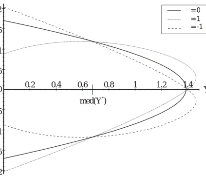
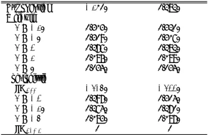
Distribution (8) is a generalization of Gumbel’s (1960) bivariate exponential distribution of the second type. There is a natural interpretation to the correlation parameterω. First, notice from (9) that ifω = 0then D∗ and Y∗ are independent. If ω >0 and both D∗ and Y∗ are above their median values, then the bracketed term adds to the likelihood. So larger than median values of D∗ and Y∗ will tend to appear together when ω is positive, and the same for smaller than median values. Figure 1 plots illustrative isoprobability curves fromfD∗,Y∗ for the case when D∗ is normal
and Y∗ is exponential. In the figure the lines represents the same probability level for different values ofω. From Figure 1, note that when either random variable is at its median,fD∗,Y∗collapses
to the product of the marginals, no matter what ω is; the curves cross at those points. When ω is negative, larger than median values of D∗ will tend to appear with smaller than median values of Y∗, and vice-versa. Thus the correlation between D∗ and Y∗ has the same sign as ω; the level varies with the specific distributions chosen. In particular, the (conditional) correlation is
ρP ≡Corr(D∗, Y∗|x, z) =ωHD∗HY∗
τ ς (11)
whereρP is Pearson’s cross-product measure of correlation andHA=−E(AGA(A)|x, z), forA = D∗, Y∗. The unconditional correlation exhibited by D∗ and Y∗ will typically be lower due to the
-2 -1.5 -1 -0.5 0 0.5 1 0.2 0.4 0.6 0.8 1 1.2 1.4
D
*Y
* 2 1.5 med(Y )* ω=-1 ω=0 ω=1Figure 1: Isoprobability curves of the generalized Gumbel distribution (D∗is normal and Y∗ is exponential)
extra noise added by the variance of the explanatory variables. When A is continuous, HA = R
FAF¯A(a)da, where the integration is over the support ofA.
The range of allowed correlation is dependent on the distributions chosen. For the exponential duration models, the allowed correlation is about(−0.3,0.3). For other duration models and count models, the correlation has (at most) the same bound, although the allowed correlation may be less depending on the parameters. Because the correlation depends on the parameters of the distributions in general, a more convenient characterization of correlation between D∗ and Y∗ is Kendall’s tau,9 which is invariant with respect toFD∗ andFY∗. Kendall’s tau measures correlation
relative to the maximally allowed correlation between two random variables, and thus is a better measure than ρP in this setting.10 No matter which marginal distributions are chosen, Kendall’s
9
Kendall’s tau is a measure of the “concordance” of two random variables, and is defined asτK ≡2 Pr{(D∗1 −
D∗
2)(Y1∗−Y2∗)>0}−1, whereAiis an independent draw fromFA,A=D∗, Y∗andi=1,2. τK is bounded between
-1 and 1 and is 0 ifD∗andY∗are independent.
1 0
tau,τK, can be shown to be
τK(D∗, Y∗|x, z) = 2
9ω (12)
for continuous marginal distributions and thus is bounded on(−2/9,2/9). By comparison, in Lee’s modelτK = (2/π) sin−1(ρ), taking values on[−1,1], a consequence of the model allowing maximal correlation (Mardia, 1970b) (see footnote 10). In sections 3 and 4 I compare the Pearson correlation allowed by the generalized Gumbel and competing models on a case by case basis.
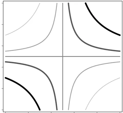
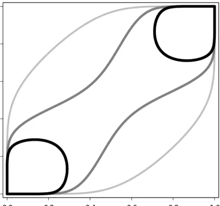
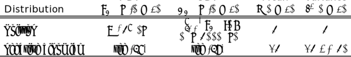
Given that the main alternative to my proposed model for continuous data is Lee’s model, it is worth comparing the correlation patterns of the two models at a deeper level than Pearson’s or Kendall’s summary statistics. For convenience, in this section I refer to the distribution underlying Lee’s model, (5), as the TBN (for Translated Bivariate Normal) distribution.11 Figures 2 and 3 plot
isoprobability curves from the generalize Gumbel and TBN distributions for the case of uniform marginals and positive correlation. Such plots, known as theuniform representation of a bivariate distribution, are convenient for comparing bivariate distributions.12 In these plots the correlation
is fixed13 and the lines represent different probability levels; thicker and darker lines represent
higher probability levels. In both plots the positive correlation has the effect of concentrating probability mass in the (0,0) and (1,1) corners. However, from the plots one can see that the generalized Gumbel distribution preserves characteristics of the original uniform marginals more than the TBN distribution. For example, when either variable takes the median value of 0.5 in the generalized Gumbel distribution, the other variable is uniformly distributed (notwithstanding the positive correlation). In the generalized Gumbel distribution, the extremal values (the borders of the unit square) are attained with positive probability, just like they are in the uniform distribution. extreme correlation (Kruskal, 1958). Pearson’sρP may be strictly inside(−1,1)at the Fréchet bounds.
1 1The TBN appears to have originated with Nataf (1962); correlation is studied by Mardia (1970b). 1 2
See Kimeldorf and Sampson (1975b) for the advantages of the uniform representation of bivariate distributions. The primary advantage is that since the uniform distribution isflat, any spikes or dips in the uniform representation are purely a consequence of correlation.
1 3
In thefigures,ω=1andρ= 0.5. The plots are qualitatively the same for any positive correlation, except that at ρ=1 all probability mass in the TBN collapses to the line y =x. Negative correlation rotates the graphs90
0.0 0.2 0.4 0.6 0.8 1.0 0.0 0.2 0.4 0.6 0.8 1.0
Figure 2: Isoprobability curves of the generalized Gumbel pdf with positive correlation (uniform representation)
In fact, the conditional distribution of one variable given the other is a straight line, with positive (negative) slope if the conditioning variable is above (below) the median. On the other hand, the TBN distribution, by construction as a translate of the bivariate normal, inherits the strong central tendencies of the normal distribution. All extremal values are attained with zero probability. The TBN distribution incorporates correlation in a fashion that makes the bivariate distribution more “normal-like,” which may be disadvantageous when the marginal distribution are chosen to reflect characteristics that are very different than those of the normal distribution–as would be the case in most duration data applications, for example.
Finally, note that one advantage of the generalized Gumbel distribution is its tractability. The additive form of the correlation terms in (8) and (9) leads to explicit analytical forms for most
0.0 0.2 0.4 0.6 0.8 1.0 0.0 0.2 0.4 0.6 0.8 1.0
Figure 3: Isoprobability curves of the generalized TBN pdf with positive correlation (uniform representation)
expressions of interest, such as the sample selection likelihood. No bivariate distribution allowing maximal correlation, that I have found, is as convenient to work with.14
2
Selection
2.1
Sample Selection
I now generalize the sample selection model, (1)—(4), using the new notation. I term the resulting model the Generalized Parametric Selection (GPS) model.The probability that D= 0is
Pr©D= 0|α0zª=FD∗(0) (13)
1 4
The likelihood of observingD= 0and Y =y is given by the integral of the joint density over the region whereY is observed:
Z ∞
0
fD∗,Y∗(t, s)dt=fY∗(y) ¯FD∗(0){1−ωFD∗(0)GY∗(y)}. (14)
From (13) and (14) the joint distribution can be written as
fD,Y(d, y) = hFD∗(0)1−dFD¯ ∗(0)d
i
[fY∗(y){1−ωFD∗(0)GY∗(y)}]d (15)
= fD(d)fY|D(y|d= 1) (16)
As seen from (16), the joint density may be decomposed into the marginal density of the binary random variableD (the first bracketed term of (15)) and the conditional density of the observed random variableY conditional on observation (the second bracketed term). The conditional density has an intuitive interpretation. When ω is positive, then Y stochastically dominates Y∗ (in the sense thatFY|D=1(y)< FY∗∗(y)∀y). 15 So the observed y is likely to be larger than the latenty∗.
The opposite holds ifω is negative. Finally, as noted above, if there is no correlation (ω= 0) then the conditional density reduces to the marginal density of Y∗.
One can calculate the conditional expectation of the observed y as:
E(y|d= 1, x, z,α,θ,ω) =µ(β0x,γ) +ωFD∗(0;α0z)HY∗(β0x,γ), (17)
whereHY∗ is as in (11). The selection term involving ω on the RHS in (17) reveals why inference
based only on the observed y’s and µ is biased. With a pairwise iid sample from fD,Y(d, y), estimation may proceed by FIML on (15), which requires no numerical integration (but see footnote 7). I use FIML in the empirical implementation of the model in section 5. However, Newey et al. (1990) note that the joint likelihood may be ill determined in practice, causing FIML to be computationally cumbersome. In such cases estimation may also proceed by LIML on fD for
1 5To see this, note that whenyis at the median ofY∗,ym, we haveG
Y∗(ym) = 0andfY|D(ym|d=1) =fY∗(ym). Forω>0and y > ym, we have fY|D(ym|d=1)> fY∗(ym). For ω>0andy < ym, we have fY|D(ym|d=1) >
ˆ
α (which will be a standard probit or logit problem) or fY|D for (ˆα,ˆθ). Two-step estimation is possible, too, although Heckman’s (1976) original method requires modification for the present case due to non-normality and the non-linearity ofµ. Equation (17) suggests a two-stage MOM or NWLS approach (along the lines of, for example, Terza, 1998). First, estimateαˆ by probit or logit. Then perform MOM onE(y|d= 1, x, z,αˆ,θ,ω) in (17) tofind (ˆθ,ωˆ). For improved efficiency, one can use the resulting (ˆα,ˆθ,ωˆ) and estimated variance to perform NWLS. The nonlinearity of the selection term implies that such two-step methods may be as computationally intensive as FIML, however, and the variance of the estimates is quite complicated in form.
2.2
Other Selection Models
The GPS model can be readily applied to other selectivity problems. For example, consider briefly the case where Y exhibits incidental truncation and D exhibits incidental censoring. For the bivariate normal distribution, Amemiya (1985) called this the Type 3 Tobit model. In particular, (4) holds as before, but (3) is replaced with
di= 1{d∗i >0}d∗i. (18)
An example of this model is where D∗ represents the number of hours worked (which is observed if greater than zero) andY∗ represents the wage. In this case we must modify (15) to be
fD,Y(d, y) = FD∗(0)1(d=0)fD∗,Y∗(d, y)1(d>0) (19) = hFD∗(0)1(d=0) i · (20) £ fD∗(d)fY∗(y)©1 +ω£¡F¯D∗−FD∗¢(d)¤ £¡F¯Y∗−FY∗¢(y)¤ª¤1(d>0)
FIML proceeds directly on (20).
The GPS model can also be applied to the non-random assignment treatment effects model (also termed the endogenous dummy variable model). In the treatment effects model, the indicator d appears as an explanatory variable in the conditional distribution ofY∗|D. Models with treatment
effects are used to evaluate the effects of job program participation on employment or wages, for example. Estimation proceeds exactly as for the sample selection model, with the inclusion ofdas one of the covariates inx.
3
Application to Duration Models
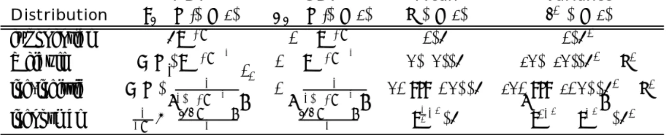
One of the main applications of the GPS model is to selection in duration models, in whichY is a subset ofR+. If one is willing to assume that the durations of interest are lognormally distributed, then one may develop a standard probit selection model based on the bivariate normal distribution. The lognormal distribution is not suitable for many applications, however, given that it exhibits a nonmonotonic hazard rate and does not admit a constant hazard rate as a special case. The other standard parametric duration models are the exponential, Weibull, and log-logistic. The densities, means, and variances of these distributions are presented in table 1. The GPS model can readily incorporate any of these, coupled with either the logit or probit form of the selection equation.
The exponential duration model is often used as a baseline model because it exhibits a constant hazard rate. From table 1 and (15) the likelihood of a sample(di, yi)from the exponential incidental truncation model is N Y i=1 h FD∗(0|zi)1−dFD¯ ∗(0|zi)d} i · (21) h e−β0xiexp ³ −y∗e−β0xi ´ n 1 +ωFD∗(0|zi) h 2 exp³−y∗e−β0xi ´ −1ioid
When D∗ is normally distributed then we have the usual probit forms FD∗(0|zi) =Φ(−α0zi) and ¯
FD∗(0|zi) = Φ(α0zi). When, instead, D∗ follows the logistic distribution, we have FD∗(0|zi) = Λ(α0zi)≡eα0zi/
³
1 +eα0zi
´
andF¯D∗(0|zi) = 1−Λ(α0zi).
What correlation is allowed? As defined in (11), we have HY∗/ς = 0.5. For probit selection,
HD∗/τ '0.564. For logit selection,HD∗/τ =√3/π '.551. Thus allowed correlation is0.282ω for
PDF CDF Mean Variance Distribution fY∗(y∗|β0x,θ) FY∗(y∗|β0x,θ) µ(β0x,θ) ς2(β0x,θ) exponential λe−λy∗ 1−e−λy∗ 1/λ 1/λ2 Weibull g(y∗)e−(λy∗)1/γ 1−e−(λy∗)1/γ γΓ(γ)/λ 2γΓ(2γ)/λ2−µ2 log-logistic g(y∗)h 1 1+(λy∗)1/γ i2 1− 1 1+(λy∗)1/γ γπcsc (πγ)/λ 2γπcsc (2πγ)/λ 2 −µ2 lognormal σ1y∗φ ³ logy∗−β0x σ ´ Φ ³ logy∗−β0x σ ´ e12σ 2 /λ ³ e2σ2−eσ2 ´ /λ2
For all models,λ=e−β0x
. φandΦare the pdf and cdf, resp., of the standard normal distribution,Γ is the Gamma function, andg(y∗) = (γy∗)−1
(λy∗)1/γ .
Table 1: Duration Distributions
Two other common duration models are the Weibull and log-logistic models. The Weibull model adds a shape parameterγ>0 to the exponential model. Whenγ= 1, the Weibull model reduces to the exponential model. Whenγ>1, the hazard is monotonically decreasing and the durations exhibit negative duration dependence. Whenγ<1, the hazard is monotonically increasing and we have positive duration dependence. The log-logistic model posits that log(y∗) follows the logistic distribution, and also has a shape parameter γ >0. The log-logistic distribution has finite mean ifγ<1 and finite variance ifγ<1/2. The hazard rate is decreasing forγ≥1and has a ∩ shape forγ <1. The allowed correlation for these models depends on the nuisance parameter γ (hence the nuisance). Table 2 lists the correlation for a few values ofγ. The correlation is about .3ω for mid-range values ofγ.
On first glance, it appears that the allowed correlation is quite limited for the various models, compared with the familiar bivariate normal distribution. However, even if one develops a bivariate duration selection model based on the normal distribution, the correlation between the duration variable and the selection variable is much less than unity in general. To be precise, consider the bivariate normal duration selection (BNDS) model, which consists of (1), (3), (4), and
Duration Logit Selection Probit Selection Exponential 0.276ω 0.282ω Weibull γ= 0.25 0.313ω 0.320ω γ= 0.5 0.309ω 0.316ω γ= 1 0.276ω 0.282ω γ= 2 0.185ω 0.189ω γ= 5 0.034ω 0.034ω Log-logistic limγ↓0 0.304ω 0.311ω γ= 0.1 0.297ω 0.304ω γ= 0.25 0.264ω 0.270ω γ= 0.4 0.183ω 0.187ω limγ↑0.5 0 0
Table 2: Allowed Correlation for the GPS Duration Models where(ui,εi) are distributed mean zero bivariate normal, with covariance matrix
Σ= σ 2 σρ σρ 1 . (23)
The BNDS model is a natural transformation of the Type 2 Tobit Model for duration data, and is in fact a special case of Lee’s model withlog(y∗i) replacingy∗i in (2), Fε =Φ in (6), andFu(ui)
= Φ(ui/σ) in (7).16 Although the transformed duration variable log(yi∗) has the full range of correlation withd∗i, the correlation betweenyi∗ andd∗i can be shown to ber(σ) =ρσ
³ eσ2−1
´−1/2
(see footnote 4).17 The correlation functionr goes to zero rapidly asσ increases. The correlation function is plotted infigure 4. The comparable correlation functions for the exponential and Weibull GPS models and Lee’s model for exponential durations (all with probit selection) are also given in
figure 4.18
The comparison reveals that the BNDS model allows for more correlation than the exponential
1 6
Most of the original labor applications of the sample selection model (e.g., Heckman, 1974) used the BNDS, although becausey∗was a wage, it was not interpreted as a duration model.
1 7
In general for Lee’s model,|corr(Y∗, D∗)|≤ρ, with equality only when(Y∗, D∗)are bivariate normal (Mardia, 1970a, p.33).
1 8The GPS correlations are functions of γ. To make them comparable to r(σ), I reparameterized them to be
functions ofδ such that log(y) has variance δ2, just as log(y) for the lognormal model has varianceσ2. For the Weibull modelδ=π/√6γ; for the log-logistic modelδ=π/√3γ. Thex-axis infigure 4 isσfor the lognormal curves andδfor the other curves.
0 0.2 0.4 0.6 0.8 1 0 0.5 1 1.5 2 2.5 3 3.5 4 σσσσ-comparable units c o rre la ti o n (s e e le gend f o r un it s ) Probit/Exponential Durations (GPS Model; units of omega) Probit/Weibull Durations (GPS Model; units of omega) Probit/Exponential Durations (Lee's Model; units of rho) Probit/Lognormal Durations (BNDS; units of rho) Probit/Log-logistic Durations (GPS Model; units of omega)
Figure 4: Comparison of allowed correlation in the duration selection models
and Weibull GPS models whenσis less than about two but admits less correlation for higher levels of σ. The log-logistic GPS model has severely limited correlation, due to the rapidity with with the variance of the log-logistic distribution approaches infinity. Lee’s model clearly allows more correlation than the GPS models. Allowed correlation is only one dimension along which to judge a model, however, and the GPS model may be preferred over Lee’s model for other reasons, which is the case in section 5.
4
Application to Count Models
The other main application of the GPS model I explore is to selection in count models, in whichY is a countably infinite subset ofR(typicallyI+). The two main parametric count models in use are the Poisson and the negative binomial. The discrete version of the GPS model can handle both,
PDF CDF Mean Variance Distribution fY∗(y∗|β0x,θ) FY∗(y∗|β0x,θ) µ(β0x,θ) ς2(β0x,θ) Poisson e−λλy∗/y∗! Py∗−1 i=0 fY∗(i) = Γ(y,λ)/Γ(y) λ λ
negative binomial see (26) see (27) γλ γλ(1 +λ)
For all models, λ= e−β0x. Γ(a) is the Gamma function andΓ(a, z) is the incomplete Gamma function,
R∞
z e−
tta−1dt.
Table 3: Distributions for Count Data
again with either the logit or probit form of the selection equation. Lee’s model does not apply to count models,19 although other parametric alternatives have been developed.
The Poisson model is the baseline model for counts because of the Markovian property of its interarrival spells, and because Poisson MLE is consistent even when the data are not generated by a Poisson process (as long as the conditional mean is correctly specified).20 The Poisson model has
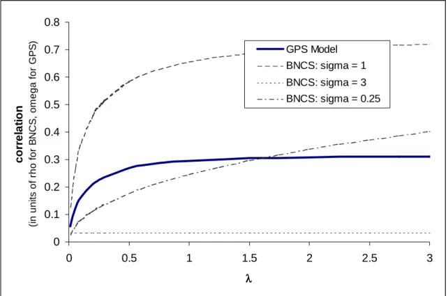
one parameter, λ=e−β0x, which is both the mean and the variance (see table 3). The likelihood of a sample(di, yi) from the incidental truncation model follows directly from (15). The selection equation may take either the logit or the probit form, as in the previous section. The allowed correlation depends onλ, starting from zero atλ= 0and converging to about 0.32ωfor the probit version asλ increases (seefigure 5).
As with the duration models and the BNDS in the previous section, a natural comparison is with a bivariate normal count selection model (BNCS).21 In the count model literature, previous
selection models have been of this type (Crepon and Duguet, 1997; Terza, 1998; Winkelmann, 1998). In particular, the model is given by (1), (3), (4), and (23), but (22) is replaced with
y∗i ∼Poisson with log(1/λi) =β0xi+ui. (24)
1 9See footnote 3. 2 0
See Cameron and Trivedi (1998) for an excellent introduction to count data modeling, estimation, and inference. For a general reference work on discrete distributions, see Johnson, Kotz and Kemp (1993).
2 1
0 0.1 0.2 0.3 0.4 0.5 0.6 0.7 0.8 0 0.5 1 1.5 2 2.5 3 λλλλ cor rel at io n (i n uni ts of r h o f o r B N C S , o m ega f o r G P S ) GPS Model BNCS: sigma = 1 BNCS: sigma = 3 BNCS: sigma = 0.25
Figure 5: Comparison of allowed correlation in the Poisson selection models The likelihood of a pairwise iid sample(di, yi)is
L(α,β) = Y di=0 Φ(−α0zi) Y di=1 Z ∞ 0 φ¡d∗i −α0zi ¢ E[f(yi|ui)|d∗i]dd∗i (25)
(see Crepon and Duguet, 1997), where f(yi|ui) is the Poisson pdf given λi = exp £
−¡β0xi+ui ¢¤
. Note that evaluation of the likelihood requires a double integration for each observation, which is computationally expensive.22 The GPS likelihood does not require integration, which makes it an
attractive alternative.
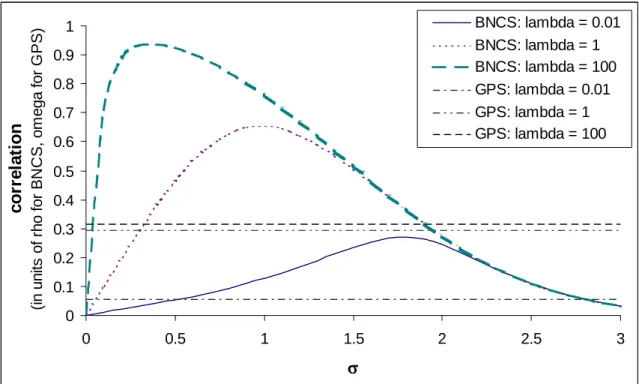
For large and small values of σ2, the GPS model allows more correlation than the Poisson BNCS model does. For intermediate values of σ2, either the Poisson BNCS model allows more correlation or the comparison depends on λ. Figure 5 also shows the correlation curves for the
2 2
0 0.1 0.2 0.3 0.4 0.5 0.6 0.7 0.8 0.9 1 0 0.5 1 1.5 2 2.5 3 σσσσ c o rre la ti o n (i n unit s of r ho fo r B N C S , om ega f o r G P S ) BNCS: lambda = 0.01 BNCS: lambda = 1 BNCS: lambda = 100 GPS: lambda = 0.01 GPS: lambda = 1 GPS: lambda = 100
Figure 6: Comparison of allowed correlation in the Poisson selection models
Poisson BNCS model, plotted for a few fixed values of σ2. Note that the shifting of the BNCS curves is not monotonic inσ2. The non-monotonicity is clearly seen in Figure 6, which plots the Poisson BNCS correlation curves as a function ofσ for a few values ofλ (and the corresponding GPS curves, for reference).
The negative binomial distribution (NBD) is another common count model that relaxes the Poisson model’s restriction that the variance equal the mean. The NBD model has pdf
fY∗(y∗|x,θ) = Γ(y+γ) Γ(y+ 1)Γ(γ) µ 1 1 +λ ¶γµ λ 1 +λ ¶y ,λ>0,γ>0 (26)
where againλ=e−β0x. The cdf may be expressed as FY∗(y∗|x,θ) = 1− Γ(y+k) Γ(y+ 1)Γ(k) µ 1 1 +λ ¶kµ λ 1 +λ ¶y 2F1 µ 1, y+k, y+ 1; λ 1 +λ ¶ , (27)
where2F1 is the hypergeometric function.23 The mean and variance depend onγ and λ(see table
2 3
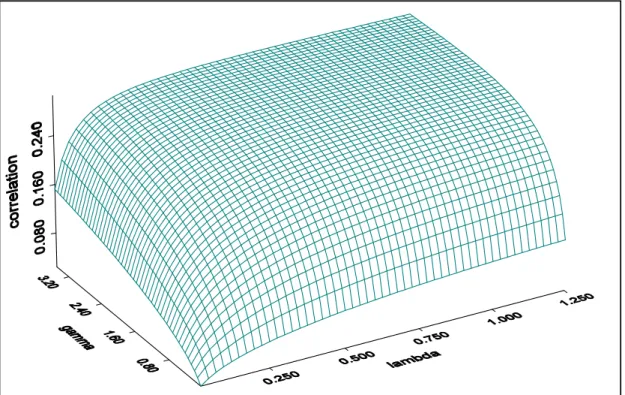
Figure 7: Allowed correlation in the GPS NBD model (in units ofω)
3). The likelihood of a sample (di, yi) from the incidental truncation model follows directly from (15), (26), and (27). The selection equation may take either the logit or the probit form, as in the previous section. The nuisance parameter adds another dimension to the correlation function; in this model the correlation depends on both γ and λ. Figure 7 shows the shape of the correlation function. Given γ, the correlation function has roughly the same shape as the GPS Poisson case (seefigure 5).
The BNCS model for the NBD distribution24 replaces (22) with
yi∗∼NBD with log(1/λi) =β0xi+ui. (28)
As with the Poisson case, it is still roughly true that for large and small values of σ2, the GPS model allows more correlation than the NBD BNCS model does. For intermediate values ofσ2, the
P∞ i=0 Γ(a+i) Γ(a) Γ(b+i) Γ(b) Γ(c) Γ(c+i)z i/i!. 2 4
Figure 8: Allowed correlation in the BNCS NBD model (in units of ρ)
comparison depends onλand γ. Figure 8 shows the correlation surface for the NBD BNCS model, where the dimension of the plot is reduced by setting γ = λ. The overall shape of the surface is about the same when plotted byfixingγorλand allowing the other to vary. In cross sections, the pattern of correlation curves are similar to the BNDS curves infigures 5 and 6.
5
An Empirical Illustration
I now demonstate the utility of the GPS model by applying it to duration data with sample se-lection. The duration data are the length of hospital stays in 1996 by participants in the Medical Expenditure Panel Survey (MEPS), a nationally representative survey of U.S. medical care and expenditures.25 The selection variable represents whether an individual had a hospital stay. Of
2 5See<http://www.meps.ahcpr.gov/>for more information on MEPS. Various data from the 1987 wave of the
survey have been studied by many authors (e.g., Madrian, 1994; Deb and Trivedi, 1997; Gilleskie, 1998). The duration of hospitalization has been previously studied by Welch (1985), Frank and Lave (1989), and Rosenman (1993).
primary interest is the effect of insurance coverage and managed care on the probability of ad-mittance to the hospital and the duration of stay. If insurance status and HMO membership are important determinants of whether an individual is hospitalized, then sample selection is an issue when analyzing the length of stay.
Three major forms of insurance are present in the sample: Medicare (MEDICARE), Medicaid (MEDICAID), and private insurance (PRIVINS) (see table 4). Medicare is available to all U.S. residents who are 65 or older. Medicare participants may also purchase additional private insurance (known as Medigap insurance). Medicaid is available to low-income individuals; most individuals on Medicaid do not have private insurance. Each of these types of coverage may be through a health maintenance organization (HMO). About half of those in the sample with private insurance are enrolled in HMOs. For Medicare and Medicaid, 22% and 38% of enrollees, respectively, are in HMOs.
HMOs are the most common form ofmanaged care plans. Managed care is a catch-all term for mechanisms that attempt to reduce the cost of health care by moving away from unrestricted fee-for-service contracts with health care providers, and may save up to one-third relative to fee-for-fee-for-service care (American Academy of Actuaries, 1996).26 Under fee-for-service contracts and marginal cost
pricing, the health care provider has the incentive to maximize the quality of care (where quality is broadly construed to include patient health, reputation of the institution, etc.), which has led to quality levels in the U.S. health care industry that have been criticized as inefficiently high. If the goal of the HMO is to reduce the quality of care (again, broadly construed), then one expects hospital stays to be less likely and shorter for individuals in HMO plans.27
Furthermore, whether the individual is insured and the type of insurance will affect the prob-ability and duration of a stay. On the demand side, since insurance greatly reduces the price of
2 6Managed care components may include limits on the length of hospital stays or full capitation, in which payment
is received per head regardless of health care usage. See Frank and Lave (1989) for a discussion of reimbursement types and the incentives they provide to health care providers.
2 7
Whether HMOs reducepatient care quality in particular is disputed. See Levinson and Ullman (1996) for an indication that infant health quality is preserved under managed care.
Insured Private Insurance Medicare Medicaid Insured 12,524 Private Insurance 10,224 10,224 Medicare 2,736 1,482 2,736 Medicaid 1,345 96 391 1,345 HMO 5,787 5,129 598 519
Table note: Cell entries are the number of individuals (out of 15,692 observations) who have insurance of both the column and the row type. An additional 150 persons were insured but not by Medicare, Medicaid, or private sources.
Table 4: MEPS Insurance Data
health care for the insured, individuals would be more likely to agree to hospitalization (when it is elective). On the supply side, health care institutions may be more willing to admit insured patients, believing that payment from uninsured patients is less likely.28 Once in the hospital, the
duration of the patient’s stay may be presumed to be up to the medical staff. Whether the hospital has incentive to release the uninsured earlier than the insured will depend on their beliefs about the probability of payment from the uninsured and the form of contract with the insurance companies for the insured. There is evidence that hospitals respond to incentives to alter their care provided based on the expected generosity of the payer (Dor and Farley, 1996).
Given that individuals are likely to take into account their future expected health when choos-ing private insurance (and to a much lesser extent Medicaid) (Ettner, 1997), I control for health status as much as possible. Medicare coverage may be considered exogenous because of its auto-matic enrollment procedure (Deb and Trivedi, 1997). I include several measures of health status reported at the beginning of the survey:29 two self-perceived measures of the individual’s health
(POORHLTH and EXCLHLTH), the number of reported medical conditions (CONDN), the
num-2 8The uninsured tend to be low wage workers who earn just enough to disqualify themselves for Medicaid. Of
those employed but earning less than $20,000 in 1996, over half were uninsured; of the uninsured, 57% worked full time (or their spouse did) (Gardner, 1997).
2 9Thefirst round of the survey took place from March to August 1996. The hospital stay data cover the entire
ber of those conditions that are on a priority list (PRIOLIST), and an indicator for disability (ADLHELP).30 The priority list contains conditions deemed important due to their prevalence,
expense, or relevance to policy, so that PRIOLIST may be viewed as a proxy for the number of severe conditions an individual has.31 Demographic variables such as region (MIDWEST, SOUTH,
WEST), sex (FEMALE),32 age (AGE),33years of education (EDUC), race (BLACK, HISPANIC),
and marriage and employment status (MARRIED, EMPLOYED) were included to capture addi-tional heterogeneity among respondents. These covariates are available for 14,955 individuals out of the 15,692 adults in the survey. A list of variables, definitions, and summary statistics is in table 5.
What is an appropriate duration model to use for the length of hospital stays? Figure 9 contains a non-parametric estimate of the baseline integrated hazard of the total hospital stays.34
The integrated hazard is linear if the hazard rate is constant, and concave if the hazard rate is declining. The figure suggests a declining hazard rate for the first few days, and a roughly constant rate after about 10 days.35 Thus an appropriate model might be the Weibull model,
which allows both declining and constant hazard rates. The lognormal andfinite-mean log-logistic distributions, with their ∩-shaped hazard rates, do not appear to be appropriate. Because the lognormal distribution is not appropriate, the BNDS model is not as attractive as the GPS or Lee
3 0
ADLHELP is a dummy variable indicating that the individual requires help or supervision carrying out Instru-mental Activities of Daily Living (IADL) or Activities of Daily Living (ADL). IADL includes using the telephone, paying bills, taking medications, preparing light meals, doing laundry, or going shopping. ADL includes personal care such as bathing, dressing, or getting around the house.
3 1
Conditions on the priority list include long-term life-threatening conditions (cancer, diabetes, emphysema, high cholesterol, HIV/AIDS, hypertension, stroke), chronic manageable conditions (arthritis, asthma, gall bladder disease, stomach ulcers, and back problems), and certain mental health conditions (Alzheimers disease, dementias, depression, and anxiety disorders).
3 2I exclude pregnancy and pregnancy-related conditions from the data set. 3 3
My sample excludes children (below 18 years of age).
3 4Points are plotted for each day that has at least one duration ending then. The estimate is from the Cox
(1972; 1975) semiparametric proportional hazards model and the Breslow’s estimate (Fleming and Harrington, 1984) of the survival curve. The Cox model takes the hazard rate to be h0(t)eβ
0x
i, whereh
0 is an unspecified baseline
hazard rate common to all individuals. The survival curve isSi(t) = exp(−Hi(t)), whereHiis the integrated hazard.
Given the Cox coefficient estimates, the survival curve is estimated, from which the baseline integrated hazard,H0(t)
=R0th0(s)ds, is recovered. The integrated hazard is plotted instead of the hazard rate becauseH0 is much smoother
thanh0.
Variable Description Mean SD HOSPSTAY Binary variable: 1=individual had hospital stay in 1996 0.09 0.28
HOSPDUR Number of nights of all hospital stays in 1996 1.19 1.07
ADLHELP 1 = requires assistance with daily living tasks 0.04 0.20
AGE Age 44.40 17.31
BLACK 1 = black (not hispanic) 0.12 0.33
CONDN Number of self-reported medical conditions 1.68 1.91
EDUC Years of education 12.38 3.16
EMPLOYED Employment status: 1=currently employed 0.65 0.48
EXCLHLTH 1 = individual reports health to be “excellent” 0.29 0.45
FEMALE 1 = female 0.54 0.50
HISPANIC 1 = of hispanic ethnicity 0.18 0.38
HMO 1 = enrolled in a health maintenance organization 0.38 0.48
MARRIED Marital status: 1 = currently married 0.57 0.49
MEDICAID 1 = currently covered by Medicaid 0.09 0.28
MEDICARE 1 = currently covered by Medicare 0.17 0.38
MIDWEST Regional indicator (EAST is the excluded dummy) 0.22 0.42
POORHLTH 1 = individual reports health to be “poor” 0.04 0.20
PRIOLIST Number of conditions on the priority list 0.54 1.00
PRIVINS 1 = covered by private insurance of any type 0.66 0.47
PRIVMCARE 1 = covered by Medicareand private insurance 0.10 0.29
SOUTH Regional indicator (EAST is the excluded dummy) 0.35 0.48
WEST Regional indicator (EAST is the excluded dummy) 0.23 0.42
days integrated hazard 0 20 40 60 80 100 02468 1 0
Figure 9: Duration of hospitalization: nonparametric estimate of the baseline integrated hazard
models in this case, which allow moreflexibility in the specification of the hazard.
In the GPS specification, the joint determination of whether an individual enters the hospital and the length of the hospital stay are allowed to be correlated through ω. Correlation between admittance and length of stay might have the following interpretation. If unobserved factors cause a person to have poorer health than average, that individual may be both more likely to enter the hospital and to need to stay longer than average, resulting in positive correlation. Negative correlation might arise a correction effect: if an individual enters the hospital when the observ-ables indicate that he should not (on average), then his condition may not be as severe as the average condition of admitted patients and the hospital stay consequently may be shorter. In this application, we have noa priori expectation on the sign of the correlation.
Baseline Model GPS Model Lee’s Model
Variable Estimate s.e. Estimate s.e. Estimate s.e.
Probit Selection PRIVINS 0.12 (0.05)∗∗ 0.12 (0.05)∗∗ 0.12 (0.05)∗∗ MEDICARE 0.28 (0.07)∗∗∗ 0.27 (0.07)∗∗∗ 0.28 (0.07)∗∗∗ MEDICAID 0.26 (0.06)∗∗∗ 0.26 (0.06)∗∗∗ 0.26 (0.06)∗∗∗ HMO 0.04 (0.04) 0.04 (0.04) 0.04 (0.04) PRIVMCARE -0.02 (0.07) -0.02 (0.07) -0.02 (0.07) CONDN 0.08 (0.01)∗∗∗ 0.08 (0.01)∗∗∗ 0.08 (0.01)∗∗∗ PRIOLIST 0.06 (0.02)∗∗∗ 0.06 (0.02)∗∗∗ 0.06 (0.02)∗∗∗ EXCLHLTH -0.14 (0.04)∗∗∗ -0.14 (0.04)∗∗∗ -0.14 (0.04)∗∗∗ POORHLTH 0.18 (0.06)∗∗∗ 0.18 (0.06)∗∗∗ 0.18 (0.06)∗∗∗ ADLHELP 0.36 (0.06)∗∗∗ 0.36 (0.06)∗∗∗ 0.36 (0.06)∗∗∗ MIDWEST 0.05 (0.05) 0.05 (0.05) 0.05 (0.05) SOUTH 0.02 (0.04) 0.01 (0.04) 0.02 (0.04) WEST -0.09 (0.05)∗ -0.10 (0.05)∗ -0.09 (0.05)∗ FEMALE 0.15 (0.03)∗∗∗ 0.14 (0.03)∗∗∗ 0.14 (0.03)∗∗∗ AGE 0.00 (0.00) 0.00 (0.00) 0.00 (0.00) BLACK -0.04 (0.05) -0.04 (0.05) -0.04 (0.05) HISPANIC 0.07 (0.05) 0.07 (0.05) 0.07 (0.05) EDUC 0.00 (0.01) 0.00 (0.01) 0.00 (0.01) MARRIED 0.06 (0.03)∗ 0.06 (0.03)∗ 0.06 (0.03)∗ EMPLOYED -0.21 (0.04)∗∗∗ -0.22 (0.04)∗∗∗ -0.21 (0.04)∗∗∗ CONSTANT -1.65 (0.11)∗∗∗ -1.64 (0.11)∗∗∗ -1.65 (0.11)∗∗∗ Exponential Durations PRIVINS 0.05 (0.07) 0.00 (0.10) 0.06 (0.09) MEDICARE -0.02 (0.10) -0.05 (0.13) -0.01 (0.11) MEDICAID 0.09 (0.09) 0.06 (0.10) 0.10 (0.09) HMO -0.13 (0.05)∗∗ -0.12 (0.07)∗ -0.13 (0.06)∗∗ PRIVMCARE -0.06 (0.11) -0.04 (0.14) -0.06 (0.12) CONDN 0.01 (0.01) -0.01 (0.02) 0.01 (0.02) PRIOLIST 0.04 (0.03) 0.04 (0.03) 0.04 (0.03) EXCLHLTH -0.01 (0.07) -0.05 (0.09) -0.01 (0.08) POORHLTH 0.43 (0.08)∗∗∗ 0.38 (0.10)∗∗∗ 0.44 (0.09)∗∗∗ ADLHELP 0.32 (0.08)∗∗∗ 0.27 (0.10)∗∗∗ 0.34 (0.09)∗∗∗ MIDWEST -0.17 (0.08)∗∗ -0.16 (0.09)∗ -0.17 (0.08)∗∗ SOUTH -0.08 (0.06) -0.07 (0.09) -0.08 (0.08) WEST -0.27 (0.07)∗∗∗ -0.26 (0.10)∗∗∗ -0.28 (0.09)∗∗∗ FEMALE -0.39 (0.06)∗∗∗ -0.37 (0.07)∗∗∗ -0.39 (0.06)∗∗∗ AGE 0.01 (0.00)∗∗∗ 0.01 (0.00)∗∗∗ 0.01 (0.00)∗∗∗ BLACK 0.19 (0.08)∗∗ 0.17 (0.10)∗ 0.19 (0.09)∗∗ HISPANIC 0.06 (0.07) 0.05 (0.09) 0.06 (0.08) EDUC 0.00 (0.01) 0.00 (0.01) 0.00 (0.01) MARRIED -0.18 (0.05)∗∗∗ -0.19 (0.07)∗∗∗ -0.18 (0.06)∗∗∗ EMPLOYED -0.21 (0.06)∗∗∗ -0.19 (0.08)∗∗ -0.22 (0.07)∗∗∗ CONSTANT 1.57 (0.17)∗∗∗ 2.05 (0.22)∗∗∗ 1.43 (0.21)∗∗∗ Corr. parameter (ω orρ) 0.88 (0.05)∗∗∗ 0.08 (0.04)∗∗
N = 14,955. * indicates 10% level significance, ** 5% level significance, and *** 1% level significance. All estimates are MLE. See table 7 for the marginal effects and table 8 for model selection criteria.
The estimation results are presented in table 6. All results presented are for probit selection and the exponential model for durations (specification testing of the Weibull model does not reject simplifying to the nested exponential model; in any case the coefficients differed little). The first estimation, presented in the first two columns, is the baseline model, in which the selection and duration equations are assumed independent. This is the equivalent of fixing ω = 0 in the GPS model (or ρ = 0 in Lee’s model). The second estimation, in columns three and four, is the GPS model with ω free, from MLE based on (21).36 The coefficient estimates are similar in the two models, although ω differs significantly from zero. The marginal effects of the covariates are presented in table 7. The major results are as follows.
• Enrollment in an HMO has no discernable effect on hospital admittance, but decreases the length of stay by 1.1 days on average (see table 7). To put thatfigure in perspective, note that the average stay was only 1.2 days. This finding is further evidence that HMO’s are successful in limiting health care expenditures and, consequently, reducing the quality of care. Expenditures are reduced by not be declining admittance but by shortening the hospitaliza-tion.
• The insurance variables (PRIVINS, MEDICARE, and MEDICAID) all increase the proba-bility of admittance to the hospital, but have no significant impact on the duration of stay. That insured individuals are more likely to receive medical care has been documented in other studies for measures such as visits to doctors’ offices (Deb and Trivedi, 1997).37 Of more novel
interest is that insured persons (under any plan) do not appear to stay in the hospital any longer or shorter than uninsured persons. Contrast this with Dor and Farley’s (1996) finding that hospitals tend to spend differing amounts on patients covered by medicare, medicaid,
3 6Since ω is restricted to the interval [
−1,1], it is computationally convenient to reparametrize as ω˜ =
Φ−1[(ω+1)/2]∈R. Standard errors reported forωin table 6 are calculated by the delta method.
3 7
Endogeneity of insurance choice would also lead to this result, if the health status controls do not adequately deal with the potential problem. Note however that the increased likelihood of hospitalization is as pronounced for MEDICAID as for the other two types of insurance, although Medicaid enrollment is exogenous.
private insurance, and not covered, depending on the generosity of the payer. This finding indicates that whether the plan is an HMO is a more important determinant of quality of care than the source (public or private) of the coverage.
• The health status controls all have expected signs in both equations. The number of med-ical and priority conditions (CONDN and PRIOLIST), disability status (ADLHELP), and self-perceived poor health (POORHLTH) all increase the probability of hospital admittance and the duration of the subsequent stay (although only the latter two are significant in the duration equation). Self-perceived good health (EXCLHLTH) has the opposite impacts.
• Some of the demographic factors affect admittance and duration of stay, but many do not. Among those with the strongest effects, employed individuals are both more likely to stay out of the hospital and to leave with shorter stays. Women are more likely to enter the hospital but have shorter stays than men. Married individuals and people in the western region have shorter stays; blacks have longer stays.
• The correlation between the selection and duration variables is significantly positive. The estimateωˆ = 0.88implies that the correlation betweenD∗ andY∗ is about 0.24 (see table 2). The positive correlation indicates that unobserved factors may make individuals both more likely to enter the hospital and to have longer stays than average (and vice versa). Note, however, that because the marginal effects of the covariates in the probit selection are small (table 7), the correlation does not much affect the marginal effects for the conditional (on observation) mean of the durations.
A final issue is the relative performance of the GPS model versus the baseline model and Lee’s model. Recall that for duration data (unlike count data, where Lee’s model is not available), both the GPS and Lee’s model can incorporate any functional form for the hazard rate, they are of comparable computational ease, but that Lee’s model allows for more correlation (see figure 4).
For comparison with the GPS model, estimates from Lee’s model (also with exponential durations) are in the last two columns of table 6. The estimates are very similar to the GPS model in general, although the correlation implied byˆρ= 0.08is only 0.07, less than one-third of the GPS estimate. Because neither the GPS model nor Lee’s model nests the other but both nest the baseline model, I use information criteria and Vuong’s test for model selection. The Akaike Information Criterion (AIC), Schwarz’s Bayesian Information Criterion (BIC), and the Consistent AIC all lead one to choose the GPS model over both Lee’s model and the baseline model.38 The BIC and consistent
AIC prefer the baseline model over Lee’s model. These information criteria are not entirely satisfactory for distinguishing between the GPS and Lee models, however, since in that case they reduce to comparing the likelihoods. A more formal guide to model selection, Vuong’s (1989) test for non-nested hypotheses, also prefers the GPS model.39 Thus the GPS model appears to be the
most appropriate model in this case.
6
Conclusion
The GPS model provides a useful alternative to Lee’s model for continuous selected variables and is moreflexible than alternatives based on the bivariate normal distribution. Although Lee’s model allows for more correlation between the selection disturbance and the selected variable, the GPS model may provide a betterfit to the data, as the application in the previous section demonstrated. The GPS model can also be used when the selected variable represents count data. Existing parametric alternatives for count data are inflexible, computationally expensive to calculate, and less tractable to work with.
3 8
The AIC (Akaike, 1974) is−2 logL+ 2k, the BIC (Schwarz, 1978) is−2 logL+klogn, and the consistent AIC (Bozdogan, 1987) is−2 logL+ (1+ logn)k, whereL is the likelihood,kis the number of parameters, and nis the number of obervations. The criteria give increasingly large penalties inkandn.
3 9These models areoverlapping, because although neither nests the other, when ω=ρ= 0they are equivalent.
To implement Vuong’s (1989) two step test for overlapping models, Ifirst reject the null hypothesis that the models are equivalent. In the present case, such rejection is immediate becauseω andρeach differ significantly from zero (Vuong, 1989, footnote 6). In the second step, the two models are discriminated based on their Kullback-Leibler information content. By this metric and using Vuong’s terminology, the GPS model is (statistically significantly) better than Lee’s model (p-value: 0.007).
Although I have not directly compared the GPS model to semiparametric approaches, the ability of the GPS model to incorporate any functional form gives it muchflexibility. For example,fY∗(y∗)
could take the “semi-nonparametric” series expansion form of Gallant and Nychka (1987) (Cameron and Johansson (1997) adapt the semi-nonparametric approach for count models). Such methods blur the distinction between parametric and semiparametric inference and lend an arbitrary amount offlexibility to maximum likelihood estimation. Another future research avenue is the application of the GPS distribution to other problems requiring bivariate distributions, such as bivariate count models, bivariate multinomial choice problems, and the like.
References
Akaike, H. (1974), ‘A New Look at the Statistical Identification Model’, IEEE Transacations on Automatic Control 19, 716—723.
Amemiya, T. (1985), Advanced Econometrics, Cambridge: Harvard University Press.
American Academy of Actuaries (1996), Medicare Managed Care: Savings, Access, and Quality, AAA, Washington, D.C.
Bozdogan, H. (1987), ‘Model Selection and Akaike’s Information Criterion (AIC): The General Theory and its Analytical Extensions’, Psychometrika52(3), 345—370.
Cameron, A. C. and Johansson, P. (1997), ‘Count Data Regression Using Series Expansions With Applications’, Journal of Applied Econometrics12, 203—223.
Cameron, A. C. and Trivedi, P. K. (1998),Regression Analysis of Count Data, Econometric Society Monographs, 30, Cambridge: Cambridge University Press.
Cox, D. R. (1972), ‘Regression Models and Life-Tables’, Journal of the Royal Statistical Society, Series B 34, 187—202.
Cox, D. R. (1975), ‘Partial Likelihood’,Biometrika 62, 269—276.
Crepon, B. and Duguet, E. (1997), ‘Research and Development, Competition and Innovation: Pseudo-Maximum Likelihood and Simulated Maximum Likelihood Methods Applied to Count Data Models with Heterogeneity’, Journal of Econometrics79(2), 355—378.
Deb, P. and Trivedi, P. K. (1997), ‘Demand for Medical Care by the Elderly: A Finite Mixture Approach’, Journal of Applied Econometrics12(3), 313—336.
Donald, S. G. (1995), ‘Two-Step Estimation of Heteroskedastic Sample Selection Models’,Journal of Econometrics 65(2), 347—380.
Dor, A. and Farley, D. E. (1996), ‘Payment Source and the Cost of Hospital Care: Evidence from a Multiproduct Cost Function With Multiple Payers’,Journal of Health Economics15(1), 453— 481.
Duncan, G. M. (1986), ‘Continuous/Descrete Econometric Models with Unspecified Error Distrib-ution’, Journal of Econometrics36, 1.
Ettner, S. L. (1997), ‘Adverse Selection and the Purchase of Medigap Insurance by the Elderly’, Journal of Health Economics 16(5), 543—562.
Fleming, T. R. and Harrington, D. P. (1984), ‘Nonparametric Estimation of the Survival Distribu-tion in Censored Data’,Communications in Statistics: Theory and Methods13(20), 2469—2486.
Frank, R. G. and Lave, J. R. (1989), ‘A Comparison of Hospital Responses to Reimbursement Policies for Medicaid Psychiatric Patients’, Rand Journal of Economics20(4), 588—600.
Gallant, A. R. and Nychka, D. W. (1987), ‘Semi-Nonparametric Maximum Likelihood Estimation’, Econometrica 55(2), 363—390.
Gilleskie, D. B. (1998), ‘A Dynamic Stochastic Model of Medical Care Use and Work Absence’, Econometrica 66(1), 1—45.
Gronau, R. (1974), ‘Wage Comparisons–A Selectivity Bias’, Journal of Political Economy 82(6), 1119—1143.
Gumbel, E. J. (1960), ‘Bivariate Exponential Distributions’, Journal of the American Statistical Association 55, 698—707.
Heckman, J. J. (1974), ‘Shadow Prices, Market Wages, and Labor Supply’, Econometrica 42(4), 679—694.
Heckman, J. J. (1976), ‘The Common Structure of Statistical Models of Truncation, Sample Selec-tion and Limited Dependent Variables and a Simple Estimator for Such Models’, Annals of Economic and Social Measurement 5, 475—492.
Johnson, N. L., Kotz, S. and Kemp, A. W. (1993),Univariate Discrete Distributions, Wiley Series in Probability and Mathematical Statistics. Probability and Mathematical Statistics, 2nd edn, New York: John Wiley & Sons.
Kimeldorf, G. and Sampson, A. R. (1975a), ‘One Parameter Families of Bivariate Distributions with Fixed Marginals’,Communications in Statistics4(3), 293—301.
Kimeldorf, G. and Sampson, A. R. (1975b), ‘Uniform Representations of Bivariate Distributions’, Communications in Statistics 4, 617—627.
Kruskal, W. H. (1958), ‘Ordinal Measures of Association’, Journal of the American Statistical Association 53(284), 814—861.
Lee, L.-F. (1983), ‘Generalized Econometric Models with Selectivity’,Econometrica51(2), 507—512. Levinson, A. and Ullman, F. (1996), ‘Medicaid Managed Care and Infant Health’,Journal of Health
Madrian, B. C. (1994), ‘Employment-Based Health Insurance and Job Mobility: Is There Evidence of Job-Lock?’, Quarterly Journal of Economics109(1), 27—54.
Manski, C. F. (1989), ‘Anatomy of the Selection Problem’,Journal of Human Resources24(3), 343— 360.
Manski, C. F. (1990), ‘Nonparametric Bounds on Treatment Effects’, American Economic Review 80(2), 319—323.
Mardia, K. V. (1970a), Families of Bivariate Distributions, Vol. 27 of Griffin’s Statistical Mono-graphs & Courses, London: Charles Griffin.
Mardia, K. V. (1970b), ‘A Translation Family of Bivariate Distributions and Fréchet’s Bounds’, Sankhy¯a A32, 119—122.
Nataf, A. (1962), ‘Déterminations Des Distributions de Probabilités Dont Les Marges Sont Don-nées’, Comptes Rendus des Séances de l’Académie des Sciences255, 42—3.
Newey, W. K., Powell, J. L. and Walker, J. R. (1990), ‘Semiparametric Estimation of Selection Models: Some Empirical Results’,American Economic Review80(2), 324—328.
Rosenman, R. E. (1993), ‘Health Plan Effects on Inpatient Resource Use: Some Contrary Evidence About IPAs’, The Journal of Socio-Economics22, 131—140.
Schwarz, G. (1978), ‘Estimating the Dimension of a Model’,Annals of Statistics 6(2), 461—464.
Stern, S. (1997), ‘Simulation-Based Estimation’,Journal of Economic Literature 35, 2006—2039.
Terza, J. V. (1998), ‘Estimating Count Data Models with Endogenous Switching: Sample Selection and Endogenous Treatment Effects’, Journal of Econometrics84(1), 129—154.
Van Ophem, H. (1999), ‘A General Method to Estimate Correlated Discrete Random Variables’, Econometric Theory 15(2), 228—237.
Vella, F. (1998), ‘Estimating Models with Sample Selection Bias: A Survey’, Journal of Human Resources 33(1), 127—169.
Vuong, Q. H. (1989), ‘Likelihood Ration Tests for Model Selection and Non-Nested Hypotheses’, Econometrica 57(2), 307—333, March.
Welch, W. P. (1985), ‘Health Care Utilization in HMO’s: Results from Two National Samples’, Journal of Health Economics 4(4), 293—308.
Winkelmann, R. (1998), ‘Count Data Models with Selectivity’,Econometric Reviews 17(4), 339— 359.
Probit Slope or ∆ Duration Slope or ∆ Variable in Pr(d= 1) in days PRIVINS 0.015 -0.003 MEDICARE 0.032 -0.462 MEDICAID 0.031 0.548 HMO 0.006 -1.130 PRIVMCARE -0.003 -0.375 CONDN 0.011 -0.072 PRIOLIST 0.008 0.374 EXCLHLTH -0.021 -0.438 POORHLTH 0.022 2.883 ADLHELP 0.039 2.163 MIDWEST 0.006 -1.564 SOUTH 0.002 -0.696 WEST -0.014 -2.693 FEMALE 0.018 -4.026 AGE 0.000 0.121 BLACK -0.005 1.449 HISPANIC 0.009 0.405 EDUC -0.001 0.019 MARRIED 0.008 -1.849 EMPLOYED -0.035 -1.880
Notes: thefigures are slopes (i.e., the derivative of the conditional mean [E(d|z)for probit,E(y|x, z, d= 1) for duration] with respect to the covariate) for continuous covariates, and discrete changes in the conditional mean for indicator variables (i.e., the change in the conditional mean when the indicator takes the value 1). The durationfigures are very similar when not conditioning on observation (i.e., for E(y|x, z) instead ofE(y|x, z, d= 1)). All figures are calculated as the average slope or change in the sample (which is more appropriate than calculating at average covariates, given the large number of dummy variables).
Selection Criterion Baseline Model GPS Model Lee’s Model Log Likelihood -7593.4 -7560.1 -7591.5 Parameters 42 43 43 Observations 14955 14955 14955 AIC 15270.8 15206.1∗ 15269.0 BIC 15590.6 15533.5∗ 15596.4 Consistent AIC 15632.6 15576.5∗ 15639.4
Vuong’s test preferred∗ not preferred
Table notes: * denotes preferred model by a particular criterion. See footnotes 38 and 39.