Procedia Computer Science 17 ( 2013 ) 1063 – 1072
1877-0509 © 2013 The Authors. Published by Elsevier B.V.
Selection and peer-review under responsibility of the organizers of the 2013 International Conference on Information Technology and Quantitative Management
doi: 10.1016/j.procs.2013.05.135
Information Technology and Quantitative Management , ITQM 2013
Nonparallel Support Vector Machines for Multiple-instance
Learning
Qin Zhang
a, Yingjie Tian
a, Dalian Liu
b,∗aResearch Center on Fictitious Economy and Data Science, Chinese Academy of Science, Beijing 100190, China bDepartment of Basic Course Teaching, Beijing Union University, Beijing 100101, China
Abstract
In this paper, we proposed a new multiple-instance learning (MIL) method based on nonparallel support vector machines (called MI-NPSVM). For the linear case, MI-NPSVM constructs two nonparallel hyperplanes by solving two SVM-type prob-lems, which is different from many other maximum margin SVM-based MIL methods. For the nonlinear case, kernel functions can be easily applied to extend the linear case, which is different from other nonparallel SVM-based MIL methods. Further-more, compared with the existing MIL method based on nonparallel SVM – MI-TSVM, MI-NPSVM has two main advantages. Firstly the method enforces the structural risk minimization; secondly it does not need to solve a bilevel programming prob-lem anymore, but to solve a series of standard Quadratic Programming Probprob-lems (QPPs). All experimental results on public datasets show that our method is superior to the traditional MIL methods like MI-SVM, MI-TSVM etc.
c
2013 The Authors. Published by Elsevier B.V.
Selection and peer-review under responsibility of the organizers of the 2013 International Conference on Information Technol-ogy and Quantitative Management.
Keywords: multiple-instance learning; support vector machine; nonparallel; classification 1. Introduction
Multiple-instance learning (MIL), which was introduced by Dietterich et al.[1] in the middle 1990’s, has received intense interests recently in the field of machine learning and been successfully applied in a wide variety of fields. In MIL framework, the training set consists of positive and negative bags of instances which are points in then-dimensional real spaceRn, and each bag contains a set of instances. In each positive training bag, there must be at least one positive instance, whereas a negative bag contains only negative instances. The aim of MIL is to construct a classifier learned from the training set to correctly label unseen bags. In a word, in MIL only the bags(but not the individual instance) have known labels, so MIL only provides weak label information of the training data. MIL has been found useful in many applications, including text categorization [2] [3], natural scene classification [4], image retrieval [4] [5], web mining [6] and so on.
Following the seminal work of Ditterich et al., a number of MIL methods were proposed, such as Diverse Density (DD)[4], EM-DD[7], mi-SVM[3], MI-SVM[3], MI-NN[5], MICA[8], SVM-CC[9]. In this paper, we
∗Corresponding author. Tel.: 010-6490-0213 ; fax: 010-6490-0213 . E-mail address:[email protected].
© 2013 The Authors. Published by Elsevier B.V.
Selection and peer-review under responsibility of the organizers of the 2013 International Conference on Information Technology and Quantitative Management
Open access under CC BY-NC-ND license.
focus on MIL methods based on Support Vector Machines, such as Andrews’ MI-SVM[3]. Inspired by the idea of nonparallel SVMs, Shao et al. proposed a MIL method called multi-instance twin support vector machines(MI-TSVM)[10], which is an extension of TWSVMs [11] and its variants[12] [13]. However, this method needs to solve a complicated bilevel programming problem, more unfortunately, its linear case can not be extended to the nonlinear via kernel functions directly, which is different with the standard SVMs.
In this paper, we propose a new multi-instance learning method based on nonparallel support vector machines, called MI-NPSVM. As the usual approach used in the nonparallel SVMs, our method finds a positive and a negative hyperplane which are nonparallel to construct the classifier of the classical MIL problem, and it has two main advantages compared with MI-TSVM. Firstly our method enforces the structural risk minimization, secondly our method does not need to solve a bilevel programming problem but to solve a series of standard Quadratic Programming Problems(QPPs).
The remaining parts of the paper are organized as follows. Section 2 gives a brief review on the twin support vector machines (TWSVMs); Section 3 describes our proposed algorithm–MI-NPSVM in detail; The solver of MI-NPSVM will be presented in Section 4; And all experimental results are presented in Section 5; Conclusions are given in the last section.
2. TWSVM
Different with standard SVMs constructing two parallel support hyperplanes, the basic idea of twin support vector machines [11] is constructing a hyperplane for each class of samples and making each hyperplane as close as possible to one class of samples, and as far as possible from the other class of samples. A new sample will be assigned to one of the classes depending upon its proximity to the two nonparallel classifier hyperplanes.
Consider a binary classification problem of classifyingm1training points belonging to class+1 andm2training
points belonging to class−1, all training points are in then-dimensional real spaceRn. For linear classification
problem, TWSVMs seeks a pair of nonparallel hyperplanes in then-dimension input space: (w+·x)+b+=0, (w−·x)+b−=0,
by solving two smaller QPPs: min w+,b+,ξ− 1 2 m1 i=1 ((w+·xi)+b+)2+C1 m1+m2 i=m1+1 ξi s.t. −((w+·xi)+b+)+ξi≥1, i=m1+1,· · ·,m1+m2, ξi≥0, i=m1+1,· · ·,m1+m2, (1) min w−,b−,ξ+ 1 2 m1+m2 i=m1+1 ((w−·xi)+b−)2+C2 m1 i=1 ξi s.t. ((w−·xi)+b−)+ξi≥1, i=1,· · ·,m1, ξi≥0, i=1,· · · ,m1, (2)
whereC1,C2are the penalty parameters,ξ+=(ξ1,· · ·, ξm1), ξ−=(ξm1+1,· · ·, ξm1+m2) are the slack variables. For nonlinear classification problem, instead of hyperplanes, two kernel-generated surfaces are considered and two other primal problems are constructed. TWSVMs have been studied extensively[14, 15, 16, 17, 18, 19, 20, 21, 22]. 3. MI-NPSVM
3.1. Linear MI-NPSVM
A) Primal Problems:Following the usual MIL methods based on Nonparallel SVMs, we construct two non-parallel hyperplanes(a positive hyperplane and a negative hyperplane)
such that, on the one hand, the positive hyperplane is close to the ”positive” instances in positive bags and is far from the all instances in negative bags, and on the other hand, the negative hyperplane is close to all instances in negative bags and is far from the ”positive” instances in positive bags. A new data pointx∈Rnis then assigned
to the positive or negative class, depending on which the hyperplane given by (3) it lies closer to, i.e.
f(x)=arg min
+,−{d+(x),d−(x)}, (4)
whered+,−(x) are the perpendicular distances:
d+(x)= |(w+·x)+b+| w+2 ,
d−(x)=|(w−·x)+b−| w−2 ,
According to the initial setting of MIL, our new method intends to make the positive classifier hyperplane cross through “the most positive instances” in positive bags, and make the negative hyperplane cross through all the negative instances in negative bags. See Figure 1 for a simple 2-dimensional linear MIL problem, there are five positive bags (instances marked by “∗”s) and five negative bags (instances marked by “◦”s). On the one hand, we hope that the most positive instances (marked by red “”) locate as near as possible to the positive straight hyperplane (w+·x)+b+ = 0 (red solid line), and push the negative bags (i.e. all the negative instances) from the straight line (w+·x)+b+ = −1 (red dotted line) as far as possible, and maximize the margin between the
hyperplanes (w+·x)+b+=0 and (w+·x)+b+=−1 in the (w+,b+)-space, which can be expressed by 1 (w+,b+). On the other hand, we hope that the negative bags (i.e. all the negative instances) locate as near as possible to the negative straight hyperplane (w−·x)+b− = 0 (blue solid line), and push the most positive instances from the straight line (w−·x)+b− = 1 (blue dotted line) as far as possible, and maximize the margin between the hyperplanes (w−·x)+b−=0 and (w−·x)+b−=1 in the (w−,b−)-space, which can be expressed by 1
(w−,b−). Based on such consideration, the two primal problems are constructed as
min w+,b+,ξ+,η− 1 2(w+ 2+b2 +)+C1 p i=1 ξ2 i +C2 r+s i=r+1 ηi (5) s.t. max j∈I(i){(w+·x i j)+b+}=ξi,i=1,· · ·,p, (6) (w+·xi)+b+≤ −1+ηi, i=r+1,· · ·,r+s, (7) ηi≥0,i=r+1,· · · ,r+s, (8) and min w−,b−,ξ−,η+ 1 2(w− 2+b2 −)+C3 r+s i=r+1 ξ2 i +C4 p i=1 ηi (9) s.t. (w−·xi)+b−=ξi, i=r+1,· · ·r+s, (10) max j∈I(i){(w−·x i j)+b−} ≥1−ηi, i=1,· · ·,p, (11) ηi≥0, i=1,· · · ,p, (12)
respectively, whereC1,C2,C3,C4≥0 are the pre-specified penalty parameters,I(i)={j|xij∈B+i},i=1,· · ·,pis
the subscript sets.
For the constraint (6), it is equivalent to that, there exists convex combination coefficients set{¯vi
j| j∈I(i),i= 1,· · ·,p}[8], such that (w+· j∈I(i) ¯ vijxij)+b+=ξi, i=1,· · ·,p, (13) j∈I(i) ¯ vij=1,v¯ij≥0,j∈I(i), i=1,· · ·,p, (14)
0 5 10 15 20 25 0 5 10 15 20 25
Fig. 1. Geometrical illustration of MI-NPSVM for a 2-dimensional linear MIL problem: 5 positive bags (instances marked by “∗”s) and 5 negative bags (instances marked by “◦”s), the most positive instances marked by red “”. Two nonparallel straight lines, (a) the red solid line crosses through the most positive instances; (b) the blue solid line crosses through all the negative instances.
Similarly, for constraint (11), there also exists convex combination coefficients{v¯¯i
j | j ∈ I(i),i = 1,· · ·,p}, such that (w−· j∈I(i) ¯¯ vijxij)+b−≥1−ηi, i=1,· · ·,p, (15) j∈I(i) ¯¯ vij=1,v¯¯ij≥0,j∈I(i), i=1,· · ·,p. (16) So the problem (5)–(8) and problem (9)–(12) are equivalent to
min w+,b+,ξ+,η−,v¯+ 1 2(w+ 2+b2 +)+C1 p i=1 ξ2 i +C2 r+s i=r+1 ηi s.t. (w+· ni j=1 ¯ vijxij)+b+=ξi, i=1,· · ·,p, (w+·xi)+b+≤ −1+ηi, i=r+1,· · · ,r+s, ni j=1 ¯ vij=1, v¯ij≥0, j=1,· · ·,ni, i=1,· · ·,p, ηi≥0, i=r+1,· · ·,r+s, (17) min w−,b−,ξ−,η+,v¯¯+ 1 2(w− 2+b2 −)+C3 r+s i=r+1 ξ2 i +C4 p i=1 ηi s.t. (w−·xi)+b−=ξi, i=r+1,· · · ,r+s, (w−· ni j=1 ¯¯ vi jxij)+b−≥1−ηi, i=1,· · · ,p, ni j=1 ¯¯ vij=1, v¯¯ij≥0, j=1,· · · ,ni, i=1,· · ·,p, ηi≥0, i=1,· · ·,p, (18)
respectively.
B)Dual problems: Obviously, problems (17) and (18) are not convex QPPs. Follow the idea of MI-SVM, an iteration method can be used to obtain their approximate solutions, which includes two strategies of updating. Since both problems have the similar formulations, so we will only discuss the problem (17) here.
(i) For fixed ¯v={v¯i
j, i=1,· · ·,p, j=1,· · ·,ni}, update (w+,b+). With the fixed ¯v, problem (17) turns to be a
standard QPP min w+,b+,ξ+,η− 1 2(w+ 2+b2 +)+C1 p i=1 ξ2 i +C2 r+s i=r+1 ηi s.t. (w+· ni j=1 ¯ vijxij)+b+=ξi, i=1,· · ·,p, (w+·xi)+b+≤ −1+ηi, i=r+1,· · ·,r+s, ηi≥0, i=r+1,· · ·,r+s. (19)
In order to get the solutions of problem (19), we need to derive it dual problem. The Lagrangian of the problem (19) is given by L(w+,b+, ξ+, η−, α+, β−, γ−)=1 2w 2 ++12b2++C1 p i=1 ξ2 i +C2 r+s i=r+1 ηi+ p i=1 αi ⎛ ⎜⎜⎜⎜⎜ ⎜⎝(w+· ni j=1 ¯ vijxij)+b+−ξi ⎞ ⎟⎟⎟⎟⎟ ⎟⎠ + r+s i=r+1 βi((w+·xi)+b++1−ηi)− r+s i=r+1 γiηi,
whereα+ =(α1,· · ·, αp) , β− =(βr+1,· · ·, βr+s) , γ− = (γr+1,· · ·, γr+s) are the Lagrange multiplier vectors.
The Karush-Kuhn-Tucker (KKT) conditions[23] forw+,b+, ξ+, η−andα+, β−, γ−are given by ∇w+L=w++ p i=1 ni j=1 αiv¯ijxij+ r+s i=r+1 βixi=0, (20) ∇b+L=b++ p i=1 αi+ r+s i=r+1 βi=0, (21) ∇ξiL=2C1ξi−αi=0, i=1,· · ·,p, (22) ∇ηiL=C2−βi−γi=0, i=r+1,· · ·,r+s, (23) (w+· ni j=1 ¯ vijxij)+b+=ξi, i=1,· · ·,p, (24) (w+·xi)+b+≤ −1+ηi, ηi≥0, i=r+1,· · ·,r+s. (25)
Sinceγ−≥0,from (23) we have
0≤β−≤C2es, (26)
whereesis a s-dimension vector with all entries are ones and in the following part it is in the same way. From
(20), (21) and (22) we have w+=− p i=1 ni j=1 αiv¯ijxij− r+s i=r+1 βixi, (27) b+=− p i=1 αi− r+s i=r+1 βi, (28) ξi= 1 2C1αi, i=1,· · ·,p, (29)
Then putting (27)–(29) into the Lagrangian and using (20)–(25), we obtain the dual problem of (19) min α+,β− 1 2 p i=1 p l=1 αiαl ⎛ ⎜⎜⎜⎜⎜ ⎜⎝ ni j=1 nl m=1 ¯ vijv¯lm(xij·xlm)+1 ⎞ ⎟⎟⎟⎟⎟ ⎟⎠+1 2 r+s i=r+1 r+s j=r+1 βiβj (xi·xj)+1 + p i=1 r+s l=r+1 αiβl ⎛ ⎜⎜⎜⎜⎜ ⎜⎝ ni j=1 ¯ vi j(xij·xl)+1 ⎞ ⎟⎟⎟⎟⎟ ⎟⎠+ 1 4C1 p i=1 α2 i − r+s i=r+1 βi s.t. 0≤β−≤C2es. (30)
Concisely, problem (30) can be further formulated as
min α+,β− 1 2α+( ¯AA¯ +E+ 1 2C1 I)α++1 2β−(BB +E)β−+α+( ¯AB +E)β−−esβ s.t. 0≤β−≤C2es, (31) whereα+ = (α1, α2,· · ·, αp) ∈ Rp, A¯ = (nj=11v¯1jx1j,· · ·, np j=1v¯ p jx p j) ∈ R p×n, B = (x r+1,· · · ,xr+s) ∈ Rs×n,
andEis the matrix of appropriate dimensions with all entries equal to one,Iis the identity matrix of appropriate dimensions. Furthermore, let ¯ π=(α+, β−) , k¯=(0,−es) ,C¯1=(−∞er,0) , C¯2=(+∞er,C2es) , and ¯ Λ = H1 H2 H2 H3 H1=A¯A¯ +E+ 1 2C1 I, H2=AB¯ +E, H3=BB +E,
therefore problem (31) is reformulated as
min ¯ π 1 2π¯ Λ¯π¯+k¯ π¯ s.t. C¯1≤π¯ ≤C¯2. (32)
(ii) For fixedw+=w¯+, the optimization problem (17) can be reduced to another convex QPP as follows min b+,ξ+,η−,v¯+ 1 2b 2 ++C1 p i=1 ξ2 i +C2 r+s i=r+1 ηi s.t. ( ¯w+· ni j=1 ¯ vijxij)+b+=ξi, i=1,· · ·,p, ( ¯w+·xi)+b+≤ −1+ηi, i=r+1,· · ·,r+s, ni j=1 ¯ vij=1, v¯ij≥0,j=1,· · ·,ni, i=1,· · ·,p, ηi≥0, i=r+1,· · ·,r+s. (33)
Similarly, problem (33) can be reformulated as min ˆ π 1 2πˆ Λˆπˆ+kˆ πˆ s.t. Hˆ1πˆ=Gˆ1, Hˆ2πˆ ≤Gˆ2, Cˆ1≤π,ˆ (34)
where ˆ π=(b+, ξ+, η−,v¯+) , kˆ=(0,0,C2es,0) , Cˆ1=(−∞ep+1,0,0) , and ˆ Λ = ⎛ ⎜⎜⎜⎜⎜ ⎜⎜⎜⎜⎜ ⎜⎜⎝ 1 0 0 0 0 2C1I 0 0 0 0 0 0 0 0 0 0 ⎞ ⎟⎟⎟⎟⎟ ⎟⎟⎟⎟⎟ ⎟⎟⎠, Hˆ1= ep −I 0 Xˆw 0 0 0 Eˆ , Gˆ1= 0 ep , ˆ H2= es 0 −I 0 , Gˆ2= −es−( ¯w B ) , ˆ Xw= ⎛ ⎜⎜⎜⎜⎜ ⎜⎜⎜⎜⎜ ⎜⎜⎜⎜⎜ ⎝ ˆ x1 w 0 · · · 0 0 xˆ2 w · · · 0 ... ... ... 0 0 · · · xˆwp ⎞ ⎟⎟⎟⎟⎟ ⎟⎟⎟⎟⎟ ⎟⎟⎟⎟⎟ ⎠ , Eˆ = ⎛ ⎜⎜⎜⎜⎜ ⎜⎜⎜⎜⎜ ⎜⎜⎜⎜⎜ ⎜⎝ en1 0 · · · 0 0 en2 · · · 0 ... ... ... 0 0 · · · enp ⎞ ⎟⎟⎟⎟⎟ ⎟⎟⎟⎟⎟ ⎟⎟⎟⎟⎟ ⎟⎠, where ˆxi w=(( ¯w+·xi1),· · ·,( ¯w+·x i
ni)) , i=1,· · · ,p.The solution of problem (33) will be used to update ¯v, further
to solve the model.
Follow the strategies of (17), problem (18) is dealt with in a similar way which is omitted here.
3.2. Nonlinear MI-NPSVM
The above discussion is restricted in the linear case. The linear approach can also be extended to construct nonlinear multi-instance classifiers by using the kernel function, such as the RBF kernel K(x,x ) =exp(−x− x 2/σ2) whereσis a real parameter. It should be pointed out that, different with MI-TWSVMs, we do not need
to consider the extra kernel-generated surfaces since only inner products appear in the dual problems, so the kernel functions can be applied directly in the problems and the linear MI-NPSVM is easily extended to the nonlinear classifier. And the iteration method discussed above can also be used to obtain its approximate solution. For the first strategy of updating, the corresponding kernel formulation of problem (30) can be expressed as
min α+,β− 1 2 p i=1 p l=1 αiαl ⎛ ⎜⎜⎜⎜⎜ ⎜⎝ ni j=1 nl m=1 ¯ vijv¯lmK(xij·xlm)+1 ⎞ ⎟⎟⎟⎟⎟ ⎟⎠+1 2 r+s i=r+1 r+s j=r+1 βiβj K(xi·xj)+1 + p i=1 r+s l=r+1 αiβl ⎛ ⎜⎜⎜⎜⎜ ⎜⎝ ni j=1 ¯ vijK(xij·xl)+1 ⎞ ⎟⎟⎟⎟⎟ ⎟⎠+ 1 4C1 p i=1 α2 i − r+s i=r+1 βi s.t. 0≤β−≤C2es. (35)
For the second strategy of updating, we can put the equation (27) obtained by the first step into the problem (33), then its corresponding kernel formulation is
min b+,ξ+,η−,v¯+ 1 2b 2 ++C1 p i=1 ξ2 i +C2 r+s i=r+1 ηi s.t. − p,ni i=1,j=1 nl m=1 αivˆ¯ijv¯lm(xij·xlm)− r+s i=r+1 nl m=1 βiv¯lm(xlm·xi)+b+=ξl,l=1,· · · ,p, − p i=1 ni j=1 αivˆ¯ij(x i j·xl)− r+s i=r+1 βi(xi·xl)+b+≤ −1+ηl,l=r+1,· · ·,r+s, ηi≥0,i=r+1,· · · ,r+s, ni j=1 ¯ vij=1,i=1,· · ·,p, ¯ vi j≥0,i=1,· · ·,p,j=1,· · ·,ni. (36)
Finally we can obtain the positive optimal hypersurface in nonlinear case, i.e. g+(x)=− p i=1 ni j=1 αivˆ¯ijK(xij·x)− r+s i=r+1 βiK(xi·x)+b+. (37) Similarly, the negative optimal hypersurface is
g−(x)= p i=1 ni j=1 βiv˜ijK(xij,x)− r+s i=r+1 αiK(xi,x)+b−. (38)
4. Fast solvers for MI-NPSVM
According to the models and formulas presented in the last section, we are able to establish the following Algorithm 1. The algorithm solving the nonlinear MI-NPSVM is very similar to that of linear MI-NPSVM which is omitted here.
Algorithm 1 Linear MI-NPSVM
Initialize: Given a training set;
Choose appropriate penalty parametersC1,C2,C3,C4>0,and appropriate parameter >0,
Setting initial values forv(1)={vi
j(1)| j=1,· · ·,ni, i=1,· · ·,p,}such as setting
vi
j(1)= n1i, j=1,· · ·,ni, i=1,· · ·,p. Process 1: 1.1For fixed ¯v(k)=v¯i
j(k), the goal is to computew−(k);
(1)Compute ¯A=(n1 j=1v¯ 1 jx1j,· · ·, np j=1v¯ p jx p j);
(2)Solve the QPP (32), obtaining the solution ¯π=(α+, β−) ; (3)Compute ¯w+from (27);
(4)Setw+(k)=w¯+;
1.2For fixedw+(k), the goal is to computev(k+1);
(1)Solve the QPP (34) with the variablesb+, ξ+, η−,v¯+, obtaining the solution ˆv=v¯+andb+;
(2)Setv(k+1)=vˆ;
1.3If|v(k+1)−v(k)|< , go to step1.4; Otherwise, goto the step1.1; setting k=k+1; 1.4Obtain the positive optimal hyperplane (w∗+·x)+b∗+=0.
Process 2: Obtain the negative optimal hyperplane (w∗−·x)+b∗−=0 similar with Process 1.
Output: For any new inputx, assign it to the classk(k= +,−) by (4), and further assign a new bag to the class.
5. Experimental Results
To demonstrate the capabilities of our algorithm, we use the same datasets and same test method as the ones in [8]. We use twelve data sets, two from the UCI machine learning repository [24], and ten from [3]. The two datasets from the UCI repository[24] are the “MUSK1” and “MUSK2” datasets, which are commonly used in multiple instance classification, involving bags of molecules and their activity levels. “Elephant”, “Fox” and “Tiger” datasets are from an image annotation task whose goal is to determine whether or not a given animal is present in an image. The other seven data sets are from the OHSUMED data and the task is to learn binary concepts associated with the Medical Subject Headings of MEDLINE documents. Detailed information about these datasets can be found in [8].
We compare MI-NPSVM with EM-DD [7], mi-SVM [3] and MI-SVM [3] for the linear case, and with MICA [8], MI-SVM [3], EM-DD [7], and SVM-CC [9], MI-TSVM [10] for the nonlinear case with RBF kernel. Exper-iment environment: Intel Core I5 CPU, 2 GB memory. The “quadprog” function in Matlab is used to solve the related optimization problems in the paper. The testing accuracies are calculated by using standard 10-fold cross validation method [25]. The regularization parametersC1,C2,C3,C4 and RBF kernel parameterσare selected
from the set{2i|i=−7,· · ·,7}by 5-fold cross validation on the tuning set comprising of random 20% of the train-ing data. Once the parameters are selected, the tuntrain-ing set is returned to the traintrain-ing set to learn the final decision function. If the difference betweenv(k+1) andv(k) is less than 10−4or the iterationk>40, the algorithms will
be stopped.
Table 1 reports the results of comparing MI-NPSVM to MI-SVM, mi-SVM, and EM-DD for the linear case. Accuracy results for mi-SVM, MI-SVM, EM-DD were taken from [3]. Obviously that MI-NPSVM has the best accuracy on “Elephant”,“Fox”,“TST2”,“TST4”,“TST7”,“TST9”,“TST10” date sets, and on the other data sets is comparable with the best accuracy of other methods.
Table 1. Ten-fold testing accuracies of methods in linear case. Best accuracy is in bold.
Data sets MI-SVM mi-SVM EM-DD MI-NPSVM Elephant 81.4% 82.2% 78.3% 83.6% Fox 57.8% 58.2% 56.1% 59.8% Tiger 84.0% 78.4% 72.1% 82.1% TST1 93.9% 93.6% 85.8% 92.8% TST2 84.5% 78.2% 84.0% 85.9% TST3 82.2% 87.0% 69.0% 84.8% TST4 82.4% 82.8% 80.5% 84.1% TST7 78.0% 81.3% 75.4% 81.5% TST9 60.2% 67.5% 65.5% 67.8% TST10 79.5% 79.6% 78.5% 80.5%
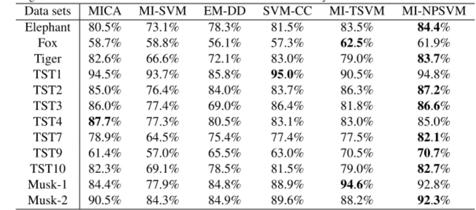
Table 2 shows the testing accuracies of some methods on the RBF kernel case, where the results for MI-SVM, EM-DD and MICA on all datasets are taken from [3] and [8] respectively. The results for SVM-CC on “Elephant”, “Tiger”, “TST1” and “Musk1” datasets are taken from [9], and the results for MI-TSVM on all datasets are taken from [10]. Our method has the best correctness on the “Elephant”, “Tiger”, “TST2”, “TST3”, “TST7”,“TST9”,“TST10” and “Musk2” and the results in other datasets are comparable with the other methods.
Table 2. Ten-fold testing accuracies of methods in the case of RBF kernel. Best accuracy is in bold.
Data sets MICA MI-SVM EM-DD SVM-CC MI-TSVM MI-NPSVM Elephant 80.5% 73.1% 78.3% 81.5% 83.5% 84.4% Fox 58.7% 58.8% 56.1% 57.3% 62.5% 61.9% Tiger 82.6% 66.6% 72.1% 83.0% 79.0% 83.7% TST1 94.5% 93.7% 85.8% 95.0% 90.5% 94.8% TST2 85.0% 76.4% 84.0% 83.7% 86.3% 87.2% TST3 86.0% 77.4% 69.0% 86.4% 81.8% 86.6% TST4 87.7% 77.3% 80.5% 83.1% 83.0% 85.0% TST7 78.9% 64.5% 75.4% 77.4% 77.5% 82.1% TST9 61.4% 57.0% 65.5% 63.0% 70.5% 70.7% TST10 82.3% 69.1% 78.5% 81.5% 79.0% 82.7% Musk-1 84.4% 77.9% 84.8% 88.9% 94.6% 92.8% Musk-2 90.5% 84.3% 84.9% 89.6% 88.2% 92.3% 6. Conclusion
A new MIL method based on nonparallel support vector machines (called MI-NPSVM) was proposed in this paper, which finds two nonparallel hyperplanes, a positive hyperplane for the positive bags and a negative hyperplane for the negative bags, by solving two SVM-type problems. Compared with other SVM-based MIL methods, it is more flexible since two nonparallel hyperplane are constructed; and more theoretically elegant since the nonlinear case can be extended from the linear case by applying kernel functions directly. The resulted two problems were efficiently solved by an iteration method, which involves solving a series of standard convex QPPs.
Experiments show that our method has better accuracies than other traditional MIL methods in most cases. In fact, MI-NPSVM also provides us a worthy MIL framework based on nonparallel classifiers. In the future work, how to use a wide variety of datasets and more effective MIL method to improve this method on better optimization and evaluation is under our consideration.
Acknowledgments
This work has been partially supported by grants from National Natural Science Foundation of China (No.11271361, No.70921061), the CAS/SAFEA International Partnership Program for Creative Research Teams, Major Interna-tional (Ragion- al) Joint Research Project (No. 71110107026), the President Fund of GUCAS.
References
[1] T. G. Dietterich, R. H. Lathrop, Solving the multiple-instance problem with axis-parallel rectangles, Artificial Intelligence 89 (1997) 31–71.
[2] O. Seref, O. E. Kundakcioglu, Multiple instance classificition with relaxed support vector machines, In Proceedings of the 3rd INFORMS Workshop on Data Mining and Health Informatics (DM-HI).
[3] S. Andrews, I. Tsochantaridis, T. Hofmann, Support vector machines for maultiple-instance learning, In Advances in Neural Information Processing Systems 15, MIT Press (2003) 561–568.
[4] O. Maron, A. L. Ratan, Multiple-instance learning for natural scene classification, In 15th International Conference on Machine Learn-ing,San Francisco, CA.
[5] J. Ramon, L. D. Raedt, Multi-instance neual networks, In Proceedings of International Conference on Machine Learning. [6] Z.-H. Zhou, K. Jiang, M. Li, Multi-instance learning based web mining, In Applied Intelligence 22(2) (2005) 135–147. [7] Q. Zhang, S. Goldman, Em-dd: an improved multiple instance learning technique, In Neural Information Processing Systems. [8] O. L. Mangasarian, E. W. Wild, Multiple instance classification via successive linear programming, Journal of Optimization Theory and
Application 137(1) (2008) 555–568.
[9] Z. X. Yang, N. Y. Deng, Multi-instance support vector machine based on convex combination, In the Eighth International Symposium on Operations Research and Its Applications (ISORA09) (2009) 481–487.
[10] Y. Shao, Z. Yang, X. Wang, N. Deng, Multiple instance twin support vector machines, In the Ninth International Symposium on Opera-tions Research and Its ApplicaOpera-tions (ISORA10) (2010) 433–442.
[11] Jayadeva, R. Khemchandani, S. Chandra, Twin support vector machines for pattern classification, IEEE Trans. Pattern Anal. Mach. Intell. 29(5) (2007) 905–910.
[12] Y. Shao, C. Zhang, X. Wang, N. Deng, Improvement on twin support machines., IEEE Transactions on Neural Networks 22(6) (2011) 962–968.
[13] Y. Shao, Z. Yang, Z. Wang, W. Chen, N. Deng, Probabilistic outputs for twin support vector machines, Knowledge Based Systems 33 (2012) 145C151.
[14] K. M. A, G. M., Application of smoothing technique on twin support vector machines., Pattern Recognit. Lett. 29(13) (2008) 1842–1848. [15] K. R, J. R. K, C. S, Optimal kernel selection in twin support vector machines, Optim. Lett. 3(1) (2009) 77–88.
[16] K. M. A, G. M, Least squares twin support vector machines for pattern classification, Expert Syst. Appl. 36(4) (2009) 7535–7543. [17] Z. Qi, Y. Tian, Y. Shi, Robust twin support vector machine for pattern classification, Pattern Recognition 46(1) (2013) 305–316. [18] Z. Qi, Y. Tian, Y. Shi, Laplacian twin support vector machine for semi-supervised classification, Neural Networks 35 (2012) 46–53. [19] Z. Qi, Y. Tian, Y. Shi, Twin support vector machine with universum data, Neural Networks 36C (2012) 112–119.
[20] Y. Tian, Y. Shi, X. Liu, Recent advances on support vector machines research, Technological and Economic Development of Economy 18(1) (2012) 5–33.
[21] N. Deng, Y. Tian, C. Zhang, Support Vector Machines–optimization based theory, algorithms, and extensions, CRC Press, 2012. [22] Y. Tian, X. Ju, Z. Qi, Efficient sparse nonparallel support vector machines for classification, Neural Computing and Applications. [23] O. Mangasarian, Nonlinear Programming, Philadelphia, PA: SIAM, 1994.
[24] P. M. Murphy, D. W. Aha, Uci machine learning repository, www.ics.uci.edu/mlearn/mlrepository.html edition. [25] T. M. Mitchell, Machine learning, McGraw-Hill International, ingapore, 1997.